The Athena Astrophysical MHD Code
in Cylindrical Geometry

M. Aaron Skinner11affiliation: askinner@astro.umd.edu and Eve C. Ostriker22affiliation: ostriker@astro.umd.edu Astronomy Department, University of Maryland, College Park, MD 20742
Abstract

A method for implementing cylindrical coordinates in the Athena magnetohydrodynamics (MHD) code is described. The extension follows the approach of Athena’s original developers and has been designed to alter the existing Cartesian-coordinates code (Stone et al., 2008) as minimally and transparently as possible. The numerical equations in cylindrical coordinates are formulated to maintain consistency with constrained transport, a central feature of the Athena algorithm, while making use of previously implemented code modules such as the Riemann solvers. Angular-momentum transport, which is critical in astrophysical disk systems dominated by rotation, is treated carefully. We describe modifications for cylindrical coordinates of the higher-order spatial reconstruction and characteristic evolution steps as well as the finite-volume and constrained transport updates. Finally, we present a test suite of standard and novel problems in one-, two-, and three-dimensions designed to validate our algorithms and implementation and to be of use to other code developers. The code is suitable for use in a wide variety of astrophysical applications and is freely available for download on the web.

hydrodynamics – MHD – methods: numerical

1 Introduction

The Athena code (Gardiner & Stone 2005, hereafter GS05; Gardiner & Stone 2008, hereafter GS08; Stone et al. 2008) is a new, second-order Godunov code for solving the equations of ideal magnetohydrodynamics (MHD). Among its salient features are that it preserves the divergence-free constraint, 𝐁=0𝐁0\nabla\cdot\mathbf{B}=0, to within machine round-off error via unsplit evolution of the magnetic field, and that it employs fully conservative updates of the MHD equations. This last feature distinguishes Athena from its predecessor, Zeus (Stone & Norman, 1992a, b), which also preserves the divergence-free constraint, but employs operator-split finite-difference methods. Athena has been extensively tested via both comparison to analytic solutions, and comparison to the results of other numerical MHD codes. The code package is freely available to the community, and is highly portable and easily configurable, as it is self-contained and does not rely on outside libraries other than MPI for computation on multi-processor distributed memory platforms.

The equations of ideal MHD consist of eight coupled partial differential equations, which are not analytically solvable in general, and fully three-dimensional numerical solutions can be quite costly. For many astrophysical systems of interest, however, the computational cost for certain problems can be reduced by exploiting geometric symmetry. For example, the high angular velocity of the plasma in accreting systems implies that most of the mass is confined within a disk. If the properties are statistically independent of azimuthal angle, ϕitalic-ϕ\phi, these disks can be studied using radial-vertical (R𝑅R-z𝑧z) models, and if vertical variations are of lesser importance, these disks can be studied using radial-azimuthal (R𝑅R-ϕitalic-ϕ\phi) models. The dynamical properties of winds and jets from astrophysical systems can also be analyzed using axisymmetric models. Exploiting symmetry in this way to reduce the effective dimension of the problem can greatly simplify the calculations involved and allow finer resolution when and where needed. In addition, for either reduced-dimensional or fully three-dimensional problems, using a curvilinear coordinate system for rotating, grid-aligned flow is superior for preservation of total angular momentum, and renders imposition of boundary conditions much simpler compared to the Cartesian-grid case.

There are several other publicly available high-resolution shock-capturing codes for astrophysical MHD in wide use, including VAC (Tóth, 1996), BATS-R-US (Powell et al., 1999), FLASH (Fryxell et al., 2000), RAMSES (Teyssier, 2002), NIRVANA (Ziegler, 2004), and PLUTO (Mignone et al., 2007), to name a few. Although these and other codes enjoy increasing popularity within the community, as of this writing only VAC and PLUTO have the capability for MHD in curvilinear coordinates.

In this paper, we describe our adaptation of Athena to support cylindrical geometry, and present a suite of tests designed to validate our algorithms and implementation. These tests include standard as well as novel problems, and may be of use to other code developers. A guiding principal of our approach is to alter the existing Athena code as minimally and as transparently as possible. This will involve a careful formulation of the MHD equations so that the finite-volume algorithm remains consistent with constrained transport, and so that the built-in Riemann solvers (as well as computation of wavespeeds and eigenfunctions) need not be changed. Finally, we pay particular attention to angular-momentum transport, which is critical in systems dominated by rotation.

The plan of this paper is as follows: In §2, we describe the conservative system of mathematical equations that we shall solve, and in §3, we briefly outline the main steps used in Athena to evolve the system numerically. In §4, we describe the projected primitive variable system used in the reconstruction step. In §§5 and 6, we describe the modifications needed for cylindrical coordinates in the higher-order spatial reconstruction and characteristic evolution steps, respectively. In §§7 and 8, we describe the implementation in cylindrical coordinates of the finite volume and constrained transport updates, respectively, and then in §9, we summarize the steps of the whole algorithm in detail. In §10, we present code verification tests and results, and we conclude in §11.

Our version of the code, including the suite of test problems we have developed, is freely available for download on the Web.

2 The Equations of MHD

The coordinate-free conservative form of the equations of ideal MHD are:

tρ+(ρ𝒗)subscript𝑡𝜌𝜌𝒗\displaystyle\partial_{t}\rho+\nabla\cdot(\rho\boldsymbol{v}) =\displaystyle= 0,0\displaystyle 0, (1a)
t(ρ𝒗)+(ρ𝒗𝒗𝑩𝑩+P𝐈)subscript𝑡𝜌𝒗𝜌𝒗𝒗𝑩𝑩superscript𝑃𝐈\displaystyle\partial_{t}(\rho\boldsymbol{v})+\nabla\cdot(\rho\boldsymbol{v}\boldsymbol{v}-\boldsymbol{B}\boldsymbol{B}+P^{*}\mathbf{I}) =\displaystyle= ρΦ,𝜌bold-∇Φ\displaystyle-\rho\,\boldsymbol{\nabla}\Phi, (1b)
tE+[(E+P)𝒗𝑩(𝑩𝒗)]subscript𝑡𝐸delimited-[]𝐸superscript𝑃𝒗𝑩𝑩𝒗\displaystyle\partial_{t}E+\nabla\cdot\left[(E+P^{*})\boldsymbol{v}-\boldsymbol{B}(\boldsymbol{B}\cdot\boldsymbol{v})\right] =\displaystyle= ρ𝒗Φ,𝜌𝒗Φ\displaystyle-\rho\,\boldsymbol{v}\cdot\nabla\Phi, (1c)
t𝑩+(𝒗𝑩𝑩𝒗)subscript𝑡𝑩𝒗𝑩𝑩𝒗\displaystyle\partial_{t}\boldsymbol{B}+\nabla\cdot(\boldsymbol{v}\boldsymbol{B}-\boldsymbol{B}\boldsymbol{v}) =\displaystyle= 0.0\displaystyle 0. (1d)

Here, ρ𝜌\rho is the mass density, ρ𝒗𝜌𝒗\rho\boldsymbol{v} is the momentum density, 𝑩𝑩\boldsymbol{B} is the magnetic field vector, and 𝐈𝐈\mathbf{I} is the identity tensor. The total pressure is defined as PP+(𝑩𝑩)/2superscript𝑃𝑃𝑩𝑩2P^{*}\equiv P+(\boldsymbol{B}\cdot\boldsymbol{B})/2, where P=nkT𝑃𝑛𝑘𝑇P=nkT is the thermal pressure, and E𝐸E is the total energy density defined as Eϵ+ρ(𝒗𝒗)/2+(𝑩𝑩)/2𝐸italic-ϵ𝜌𝒗𝒗2𝑩𝑩2E\equiv\epsilon+\rho(\boldsymbol{v}\cdot\boldsymbol{v})/2+(\boldsymbol{B}\cdot\boldsymbol{B})/2, where ϵitalic-ϵ\epsilon is the internal energy density. An ideal gas equation of state P=(γ1)ϵ𝑃𝛾1italic-ϵP=(\gamma-1)\epsilon is assumed, where γ𝛾\gamma is the ratio of specific heats. As written, the equations have been scaled in such a way that the magnetic permeability is μ=1𝜇1\mu=1 (for cgs units, 𝑩𝑩\boldsymbol{B} is replaced by 𝑩/4π𝑩4𝜋\boldsymbol{B}/\sqrt{4\pi}). Optionally, we can include a static gravitational potential Φ=Φ(𝒙)ΦΦ𝒙\Phi=\Phi(\boldsymbol{x}) in equations (1b) and (1c); the energy equation (1c) can also be generalized by including radiative heating and cooling terms.

Ignoring terms on the right-hand sides, equations (1) can be summarized by the single evolution equation in “conservative” form:

t𝑸+𝑭=0,subscript𝑡𝑸𝑭0\partial_{t}\boldsymbol{Q}+\nabla\cdot\boldsymbol{F}=0, (2)

where 𝑸=𝑸(𝒙,t)𝑸𝑸𝒙𝑡\boldsymbol{Q}=\boldsymbol{Q}(\boldsymbol{x},t) is the set of conserved quantities

𝑸(ρρ𝒗E𝑩),𝑸𝜌𝜌𝒗𝐸𝑩\boldsymbol{Q}\equiv\left(\begin{array}[]{c}\rho\\ \rho\boldsymbol{v}\\ E\\ \boldsymbol{B}\end{array}\right), (3)

and

𝐅[ρ𝒗𝐌(E+P)𝒗𝑩(𝒗𝑩)𝐉]𝐅delimited-[]𝜌𝒗𝐌𝐸superscript𝑃𝒗𝑩𝒗𝑩𝐉\mathbf{F}\equiv\left[\begin{array}[]{c}\rho\boldsymbol{v}\\ \mathbf{M}\\ (E+P^{*})\boldsymbol{v}-\boldsymbol{B}(\boldsymbol{v}\cdot\boldsymbol{B})\\ \mathbf{J}\end{array}\right] (4)

is a structure whose components represent the (nonlinear) fluxes associated with the various components of 𝑸𝑸\boldsymbol{Q}. For added simplicity, we have defined the momentum and induction tensors:

𝐌ρ𝒗𝒗𝑩𝑩+P𝐈,𝐌𝜌𝒗𝒗𝑩𝑩superscript𝑃𝐈\mathbf{M}\equiv\rho\boldsymbol{v}\boldsymbol{v}-\boldsymbol{B}\boldsymbol{B}+P^{*}\mathbf{I}, (5)

and

𝐉𝒗𝑩𝑩𝒗.𝐉𝒗𝑩𝑩𝒗\mathbf{J}\equiv\boldsymbol{v}\boldsymbol{B}-\boldsymbol{B}\boldsymbol{v}. (6)

Note that additional terms such as gravitational forces appearing on the right-hand sides of equations (1) are treated separately as source terms, hence are not part of the conservative system in equation (2).

In Cartesian coordinates, equation (2) can be expanded in a straightforward manner:

t𝑸+x𝑭x+y𝑭y+z𝑭z=0,subscript𝑡𝑸subscript𝑥subscript𝑭𝑥subscript𝑦subscript𝑭𝑦subscript𝑧subscript𝑭𝑧0\partial_{t}\boldsymbol{Q}+\partial_{x}\boldsymbol{F}_{x}+\partial_{y}\boldsymbol{F}_{y}+\partial_{z}\boldsymbol{F}_{z}=0, (7)

where 𝑭xsubscript𝑭𝑥\boldsymbol{F}_{x}, 𝑭ysubscript𝑭𝑦\boldsymbol{F}_{y}, and 𝑭zsubscript𝑭𝑧\boldsymbol{F}_{z} are one-dimensional vectors representing the fluxes of various components of 𝑸𝑸\boldsymbol{Q} in each orthogonal coordinate direction.

In order to extend the existing algorithm in Athena to curvilinear coordinates, we introduce geometric scale factors and source terms arising from the covariant derivatives in the curved metric. Following this approach, the existing code can be made to support cylindrical geometry with only moderate adjustments, which is what we describe in this paper.

We expand equation (2) according to the form of the divergence operator in cylindrical coordinates (see e.g. Mihalas & Mihalas, 1984) when acting on a vector,

𝒗=1RR(RvR)+1Rϕvϕ+zvz,𝒗1𝑅subscript𝑅𝑅subscript𝑣𝑅1𝑅subscriptitalic-ϕsubscript𝑣italic-ϕsubscript𝑧subscript𝑣𝑧\nabla\cdot\boldsymbol{v}=\text@frac{1}{R}\partial_{R}\left(R\,v_{R}\right)+\text@frac{1}{R}\partial_{\phi}v_{\phi}+\partial_{z}v_{z}, (8)

and when acting on a tensor,

(𝐓)Rsubscript𝐓𝑅\displaystyle(\nabla\cdot\mathbf{T})_{R} =\displaystyle= 1RR(RTRR)+1RϕTϕR+zTzR1RTϕϕ1𝑅subscript𝑅𝑅subscript𝑇𝑅𝑅1𝑅subscriptitalic-ϕsubscript𝑇italic-ϕ𝑅subscript𝑧subscript𝑇𝑧𝑅1𝑅subscript𝑇italic-ϕitalic-ϕ\displaystyle\text@frac{1}{R}\partial_{R}\left(R\,T_{RR}\right)+\text@frac{1}{R}\partial_{\phi}T_{\phi R}+\partial_{z}T_{zR}-\text@frac{1}{R}T_{\phi\phi} (9a)
(𝐓)ϕsubscript𝐓italic-ϕ\displaystyle(\nabla\cdot\mathbf{T})_{\phi} =\displaystyle= 1RR(RTRϕ)+1RϕTϕϕ+zTzϕ+1RTϕR1𝑅subscript𝑅𝑅subscript𝑇𝑅italic-ϕ1𝑅subscriptitalic-ϕsubscript𝑇italic-ϕitalic-ϕsubscript𝑧subscript𝑇𝑧italic-ϕ1𝑅subscript𝑇italic-ϕ𝑅\displaystyle\text@frac{1}{R}\partial_{R}\left(R\,T_{R\phi}\right)+\text@frac{1}{R}\partial_{\phi}T_{\phi\phi}+\partial_{z}T_{z\phi}+\text@frac{1}{R}T_{\phi R} (9b)
(𝐓)zsubscript𝐓𝑧\displaystyle(\nabla\cdot\mathbf{T})_{z} =\displaystyle= 1RR(RTRz)+1RϕTϕz+zTzz.1𝑅subscript𝑅𝑅subscript𝑇𝑅𝑧1𝑅subscriptitalic-ϕsubscript𝑇italic-ϕ𝑧subscript𝑧subscript𝑇𝑧𝑧\displaystyle\text@frac{1}{R}\partial_{R}\left(R\,T_{Rz}\right)+\text@frac{1}{R}\partial_{\phi}T_{\phi z}+\partial_{z}T_{zz}. (9c)

The extra non-derivative terms in equations (9a) and (9b) are the so-called geometric source terms, and represent “fictitious” forces, e.g. the centrifugal and Coriolis forces. Once source terms are introduced, the finite-volume updates are no longer fully conservative. As we shall next show, however, all but one of the geometric source terms can be eliminated from the equations. This remaining geometric source term, appearing in the radial momentum equation, is often balanced by gravity in realistic astrophysical problems.

2.1 Continuity Equation

Expanding the derivative operators in cylindrical coordinates in equation (1a), we have the continuity equation in conservative variable form:

tρ+1RR(RρvR)+1Rϕ(ρvϕ)+z(ρvz)=0.subscript𝑡𝜌1𝑅subscript𝑅𝑅𝜌subscript𝑣𝑅1𝑅subscriptitalic-ϕ𝜌subscript𝑣italic-ϕsubscript𝑧𝜌subscript𝑣𝑧0\partial_{t}\rho+\text@frac{1}{R}\partial_{R}(R\,\rho v_{R})+\text@frac{1}{R}\partial_{\phi}(\rho v_{\phi})+\partial_{z}(\rho v_{z})=0. (10)

2.2 Momentum Equation

For the momentum equation (1b), we have, in terms of the symmetric momentum tensor 𝐌𝐌\mathbf{M} (eq. 5):

t(ρvR)+1RR(RMRR)+1RϕMϕR+zMzRsubscript𝑡𝜌subscript𝑣𝑅1𝑅subscript𝑅𝑅subscript𝑀𝑅𝑅1𝑅subscriptitalic-ϕsubscript𝑀italic-ϕ𝑅subscript𝑧subscript𝑀𝑧𝑅\displaystyle\partial_{t}(\rho v_{R})+\text@frac{1}{R}\partial_{R}(R\,M_{RR})+\text@frac{1}{R}\partial_{\phi}M_{\phi R}+\partial_{z}M_{zR} =\displaystyle= 1RMϕϕ1𝑅subscript𝑀italic-ϕitalic-ϕ\displaystyle\text@frac{1}{R}M_{\phi\phi} (11a)
t(ρvϕ)+1RR(RMRϕ)+1RϕMϕϕ+zMzϕsubscript𝑡𝜌subscript𝑣italic-ϕ1𝑅subscript𝑅𝑅subscript𝑀𝑅italic-ϕ1𝑅subscriptitalic-ϕsubscript𝑀italic-ϕitalic-ϕsubscript𝑧subscript𝑀𝑧italic-ϕ\displaystyle\partial_{t}(\rho v_{\phi})+\text@frac{1}{R}\partial_{R}(R\,M_{R\phi})+\text@frac{1}{R}\partial_{\phi}M_{\phi\phi}+\partial_{z}M_{z\phi} =\displaystyle= 1RMϕR1𝑅subscript𝑀italic-ϕ𝑅\displaystyle-\text@frac{1}{R}M_{\phi R} (11b)
t(ρvz)+1RR(RMRz)+1RϕMϕz+zMzzsubscript𝑡𝜌subscript𝑣𝑧1𝑅subscript𝑅𝑅subscript𝑀𝑅𝑧1𝑅subscriptitalic-ϕsubscript𝑀italic-ϕ𝑧subscript𝑧subscript𝑀𝑧𝑧\displaystyle\partial_{t}(\rho v_{z})+\text@frac{1}{R}\partial_{R}(R\,M_{Rz})+\text@frac{1}{R}\partial_{\phi}M_{\phi z}+\partial_{z}M_{zz} =\displaystyle= 0.0\displaystyle 0. (11c)

Mignone et al. (2007) note that the symmetric character of 𝐌𝐌\mathbf{M} allows further simplification of equation (11b) in cylindrical coordinates, since

(𝐌)ϕ=1R2R(R2MRϕ)+1RϕMϕϕ+zMzϕ.subscript𝐌italic-ϕ1superscript𝑅2subscript𝑅superscript𝑅2subscript𝑀𝑅italic-ϕ1𝑅subscriptitalic-ϕsubscript𝑀italic-ϕitalic-ϕsubscript𝑧subscript𝑀𝑧italic-ϕ(\nabla\cdot\mathbf{M})_{\phi}=\text@frac{1}{R^{2}}\partial_{R}(R^{2}\,M_{R\phi})+\text@frac{1}{R}\partial_{\phi}M_{\phi\phi}+\partial_{z}M_{z\phi}. (12)

This leads to the so-called “angular momentum-conserving form” of the ϕitalic-ϕ\phi-momentum equation:

t(ρRvϕ)+1RR(R2MRϕ)+1Rϕ(RMϕϕ)+z(RMzϕ)=0subscript𝑡𝜌𝑅subscript𝑣italic-ϕ1𝑅subscript𝑅superscript𝑅2subscript𝑀𝑅italic-ϕ1𝑅subscriptitalic-ϕ𝑅subscript𝑀italic-ϕitalic-ϕsubscript𝑧𝑅subscript𝑀𝑧italic-ϕ0\partial_{t}(\rho\,R\,v_{\phi})+\text@frac{1}{R}\partial_{R}(R^{2}\,M_{R\phi})+\text@frac{1}{R}\partial_{\phi}(R\,M_{\phi\phi})+\partial_{z}(R\,M_{z\phi})=0 (13)

Note that in this form, the conserved quantity is angular momentum and there is no source term. However, since the original Cartesian version of Athena makes use of linear momenta in the flux calculations and since we do not wish to alter those calculations, we rewrite this equation once more to obtain the ϕitalic-ϕ\phi-momentum equation that we shall use:

t(ρvϕ)+1R2R(R2MRϕ)+1RϕMϕϕ+zMzϕ=0.subscript𝑡𝜌subscript𝑣italic-ϕ1superscript𝑅2subscript𝑅superscript𝑅2subscript𝑀𝑅italic-ϕ1𝑅subscriptitalic-ϕsubscript𝑀italic-ϕitalic-ϕsubscript𝑧subscript𝑀𝑧italic-ϕ0\partial_{t}(\rho\,v_{\phi})+\text@frac{1}{R^{2}}\partial_{R}(R^{2}\,M_{R\phi})+\text@frac{1}{R}\partial_{\phi}M_{\phi\phi}+\partial_{z}M_{z\phi}=0. (14)

This leaves the term Mϕϕ/R=(ρvϕ2Bϕ2+P)/Rsubscript𝑀italic-ϕitalic-ϕ𝑅𝜌superscriptsubscript𝑣italic-ϕ2superscriptsubscript𝐵italic-ϕ2superscript𝑃𝑅M_{\phi\phi}/R=(\rho v_{\phi}^{2}-B_{\phi}^{2}+P^{*})/R appearing in the R𝑅R-momentum equation (11a) as the only geometric source term in the cylindrical coordinate expansion of equation (1b). In practice, this source term is often (partially) balanced by the radial component of the gravitational source term

ρΦ𝜌bold-∇Φ-\rho\,\boldsymbol{\nabla}\Phi (15)

for many astrophysical applications.

2.3 Energy Equation

For the total energy equation (1c) in conservative form, we have

tEsubscript𝑡𝐸\displaystyle\partial_{t}E +\displaystyle+ 1RR[R((E+P)vRBR(𝑩𝒗))]+1Rϕ((E+P)vϕBϕ(𝑩𝒗))1𝑅subscript𝑅delimited-[]𝑅𝐸superscript𝑃subscript𝑣𝑅subscript𝐵𝑅𝑩𝒗1𝑅subscriptitalic-ϕ𝐸superscript𝑃subscript𝑣italic-ϕsubscript𝐵italic-ϕ𝑩𝒗\displaystyle\text@frac{1}{R}\partial_{R}\left[R\,((E+P^{*})v_{R}-B_{R}\,(\boldsymbol{B}\cdot\boldsymbol{v}))\right]+\text@frac{1}{R}\partial_{\phi}((E+P^{*})v_{\phi}-B_{\phi}(\boldsymbol{B}\cdot\boldsymbol{v})) (16)
+\displaystyle+ z((E+P)vzBz(𝑩𝒗))=0.subscript𝑧𝐸superscript𝑃subscript𝑣𝑧subscript𝐵𝑧𝑩𝒗0\displaystyle\partial_{z}((E+P^{*})v_{z}-B_{z}(\boldsymbol{B}\cdot\boldsymbol{v}))=0.

The gravitational source term for the energy equation is

ρ𝒗Φ.𝜌𝒗bold-∇Φ-\rho\,\boldsymbol{v}\cdot\boldsymbol{\nabla}\Phi. (17)

2.4 Induction Equation

Finally, for the induction equation (1d), we have in terms of the antisymmetric induction tensor, 𝐉𝐉\mathbf{J} (eq. 6):

tBR+1RϕJϕR+zJzRsubscript𝑡subscript𝐵𝑅1𝑅subscriptitalic-ϕsubscript𝐽italic-ϕ𝑅subscript𝑧subscript𝐽𝑧𝑅\displaystyle\partial_{t}B_{R}+\text@frac{1}{R}\partial_{\phi}J_{\phi R}+\partial_{z}J_{zR} =\displaystyle= 00\displaystyle 0 (18a)
tBϕ+1RR(RJRϕ)+zJzϕsubscript𝑡subscript𝐵italic-ϕ1𝑅subscript𝑅𝑅subscript𝐽𝑅italic-ϕsubscript𝑧subscript𝐽𝑧italic-ϕ\displaystyle\partial_{t}B_{\phi}+\text@frac{1}{R}\partial_{R}(R\,J_{R\phi})+\partial_{z}J_{z\phi} =\displaystyle= JRϕRsubscript𝐽𝑅italic-ϕ𝑅\displaystyle\text@frac{J_{R\phi}}{R} (18b)
tBz+1RR(RJRz)+1RϕJϕzsubscript𝑡subscript𝐵𝑧1𝑅subscript𝑅𝑅subscript𝐽𝑅𝑧1𝑅subscriptitalic-ϕsubscript𝐽italic-ϕ𝑧\displaystyle\partial_{t}B_{z}+\text@frac{1}{R}\partial_{R}(R\,J_{Rz})+\text@frac{1}{R}\partial_{\phi}J_{\phi z} =\displaystyle= 0.0\displaystyle 0. (18c)

It is important for the preservation of the divergence constraint that we avoid source terms in the magnetic fluxes. Thus, we rewrite the ϕitalic-ϕ\phi-induction equation (18b) as

t(BϕR)+1RR(RJRϕR)+z(JzϕR)=0.subscript𝑡subscript𝐵italic-ϕ𝑅1𝑅subscript𝑅𝑅subscript𝐽𝑅italic-ϕ𝑅subscript𝑧subscript𝐽𝑧italic-ϕ𝑅0\partial_{t}\left(\text@frac{B_{\phi}}{R}\right)+\text@frac{1}{R}\partial_{R}\left(R\,\text@frac{J_{R\phi}}{R}\right)+\partial_{z}\left(\text@frac{J_{z\phi}}{R}\right)=0. (19)

Note that in this form, the conserved quantity is Bϕ/Rsubscript𝐵italic-ϕ𝑅B_{\phi}/R and there is no source term. Equation (19) has also modified the fluxes of Bϕsubscript𝐵italic-ϕB_{\phi}, but since Athena does not actually use flux differences to evolve the magnetic fields (see §8), this is not a serious problem. We will use a reduced form equivalent to equation (19) for Bϕsubscript𝐵italic-ϕB_{\phi} in the reconstruction step (see §4):

tBϕ+RJRϕ+zJzϕ=0.subscript𝑡subscript𝐵italic-ϕsubscript𝑅subscript𝐽𝑅italic-ϕsubscript𝑧subscript𝐽𝑧italic-ϕ0\partial_{t}B_{\phi}+\partial_{R}J_{R\phi}+\partial_{z}J_{z\phi}=0. (20)

In this form, we use the fluxes JRϕsubscript𝐽𝑅italic-ϕJ_{R\phi} and Jzϕsubscript𝐽𝑧italic-ϕJ_{z\phi} originally appearing in equation (18b), not the modified fluxes JRϕ/Rsubscript𝐽𝑅italic-ϕ𝑅J_{R\phi}/R and Jzϕ/Rsubscript𝐽𝑧italic-ϕ𝑅J_{z\phi}/R appearing in equation (19).

3 Overview of the Numerical Algorithm

The algorithm used in Athena to evolve the system in equation (2) uses a Godunov-type finite volume (FV) scheme. A simplified version of the algorithm presented in Stone et al. (2008) is as follows:

  1. 1.

    Using cell-centered volume averages at time tnsuperscript𝑡𝑛t^{n}, compute left and right (L/R) interface states with the reconstruct-evolve-average (REA) method based on the linearized one-dimensional evolution equations.

  2. 2.

    Add the parallel components of source terms to the L/R states.

  3. 3.

    Compute the first-order interface fluxes from the L/R states using an exact or approximate Riemann solver.

  4. 4.

    Update the L/R states’ magnetic fields using constrained transport (CT) (Evans & Hawley, 1988).

  5. 5.

    Correct the L/R states’ remaining non-magnetic variables with transverse flux gradients and the transverse components of source terms.

  6. 6.

    Compute the second-order interface fluxes from the corrected L/R states using the Riemann solver.

  7. 7.

    Using the second-order fluxes, advance the interface magnetic fields to time tn+1=t+Δtsuperscript𝑡𝑛1𝑡Δ𝑡t^{n+1}=t+\Delta t with CT.

  8. 8.

    Using the second-order fluxes, advance the remaining cell-centered quantities to time tn+1superscript𝑡𝑛1t^{n+1} with the FV method.

  9. 9.

    Add the time- and volume-averaged source terms to the cell-centered quantities.

  10. 10.

    Average the interface magnetic field components to obtain the cell-centered field components at time tn+1superscript𝑡𝑛1t^{n+1}.

  11. 11.

    Compute a new timestep ΔtΔ𝑡\Delta t based on the CFL condition and repeat steps (1)-(11) until tn+1tfsuperscript𝑡𝑛1subscript𝑡𝑓t^{n+1}\geq t_{f}.

Currently, Athena includes a wide variety of non-linear Riemann solvers (see Stone et al., 2008, for a complete list). In our tests, we use the solvers based on the HLL flux (Harten et al., 1983) as well as Roe’s linearized method (Roe, 1981). Among the solvers based on the HLL flux are the HLLE solver (Einfeldt et al., 1991), which uses a single intermediate state, the HLLC solver (Toro, 1999), which extends the original HLLE solver by including a contact wave, and the HLLD solver (Miyoshi & Kusano, 2005), which extends the original HLLE solver by including both contact and Alfvén waves. The HLLE solver has the advantage that it is simple and therefore faster than more accurate solvers such as Roe’s method, and like all solvers based on the HLL fluxes, it is positive-definite for 1D problems. However, since it neglects the contact wave, and additionally the Alfvén waves for MHD, it is overly-diffusive for these waves. On the other hand, for hydrodynamics, the HLLC solver produces fluxes that are as accurate, if not better, than those produced by Roe’s method, but at a considerably lower computational cost. For MHD, it has been shown that the HLLD solver is of comparable accuracy to the MHD extension of Roe’s method for several tests using Athena, although it is much faster (Stone et al., 2008). The advantage of Roe’s linearized method is that it includes all waves in a given problem, yielding less diffusive and, hence, more accurate results for intermediate waves that are neglected by the methods based on HLL fluxes, although for some values of the left and right states, Roe’s method will fail to return positive density and/or pressure in the intermediate state(s). Finally, we reiterate that with the approach we have adopted, it is not necessary to make any changes to the computation of wavespeeds, eigenfunctions, or fluxes in any of these methods.

Although no changes are required for the solution of the Riemann problem at interfaces, several changes are required in other parts of the Athena algorithm in order to accommodate non-Cartesian coordinates. In the next sections, we discuss the geometry-specific details of computing the L/R states (steps 1-2; see §§4-6), the FV method (steps 8-9; see §7), and the incorporation of CT into the corner transport upwind (CTU) method of Colella (1990) (see §8). Finally, we will recapitulate the steps of the algorithm in greater detail and explain the computation of the new timestep (step 11; see §9).

4 The Linearized Evolution Equations

In Athena, the left and right (L/R) interface states (the inputs to the Riemann solver) are computed using a modified form of the system in equation (2). The equations, written in primitive variable form, are projected in a single coordinate direction, and the resulting system is linearized and then evolved. The projection in the ϕitalic-ϕ\phi-direction yields a system that can be obtained from the corresponding Cartesian projection (see GS05, §3.1) by making the substitution yR1ϕmaps-tosubscript𝑦superscript𝑅1subscriptitalic-ϕ\partial_{y}\mapsto R^{-1}\partial_{\phi}. However, the projection in the R𝑅R-direction differs more significantly as a result of geometric scale factors.

For the projection in the R𝑅R-direction, we begin with the primitive variable form of equation (2), take ϕ0subscriptitalic-ϕ0\partial_{\phi}\equiv 0 and z0subscript𝑧0\partial_{z}\equiv 0, expand the remaining R𝑅R-partials, and move the non-derivative terms to the right-hand side to obtain the system:

t𝒘+𝐀R𝒘=𝒔,subscript𝑡𝒘𝐀subscript𝑅𝒘𝒔\partial_{t}\boldsymbol{w}+\mathbf{A}\partial_{R}\boldsymbol{w}=\boldsymbol{s}, (21)

where

𝒘=[ρvRvϕvzPBϕBz]𝒘delimited-[]𝜌subscript𝑣𝑅subscript𝑣italic-ϕsubscript𝑣𝑧𝑃subscript𝐵italic-ϕsubscript𝐵𝑧\boldsymbol{w}=\left[\begin{array}[]{c}\rho\\ v_{R}\\ v_{\phi}\\ v_{z}\\ P\\ B_{\phi}\\ B_{z}\end{array}\right] (22)

is the vector of primitive variables, omitting the parallel component of the magnetic field,

𝐀=[vRρ000000vR001/ρBϕ/ρBz/ρ00vR00BR/ρ0000vR00BR/ρ0γP00vR000BϕBR00vR00Bz0BR00vR]𝐀delimited-[]subscript𝑣𝑅𝜌000000subscript𝑣𝑅001𝜌subscript𝐵italic-ϕ𝜌subscript𝐵𝑧𝜌00subscript𝑣𝑅00subscript𝐵𝑅𝜌0000subscript𝑣𝑅00subscript𝐵𝑅𝜌0𝛾𝑃00subscript𝑣𝑅000subscript𝐵italic-ϕsubscript𝐵𝑅00subscript𝑣𝑅00subscript𝐵𝑧0subscript𝐵𝑅00subscript𝑣𝑅\mathbf{A}=\left[\begin{array}[]{ccccccc}v_{R}&\rho&0&0&0&0&0\\ 0&v_{R}&0&0&1/\rho&B_{\phi}/\rho&B_{z}/\rho\\ 0&0&v_{R}&0&0&-B_{R}/\rho&0\\ 0&0&0&v_{R}&0&0&-B_{R}/\rho\\ 0&\gamma P&0&0&v_{R}&0&0\\ 0&B_{\phi}&-B_{R}&0&0&v_{R}&0\\ 0&B_{z}&0&-B_{R}&0&0&v_{R}\end{array}\right] (23)

is the wave matrix, and 𝒔=𝒔MHD+𝒔grav+𝒔geom𝒔subscript𝒔MHDsubscript𝒔gravsubscript𝒔geom\boldsymbol{s}=\boldsymbol{s}_{\rm MHD}+\boldsymbol{s}_{\rm grav}+\boldsymbol{s}_{\rm geom} is the source term vector, a combination of the MHD source terms arising from the 𝑩𝑩\nabla\cdot\boldsymbol{B} constraint, gravity source terms from a static potential, and the geometric source terms inherent in the cylindrical coordinate system. As in the Cartesian version of Athena, the form of the MHD source terms differs slightly in the 2D and 3D cases (see §4.4 below), but the forms of the gravity and geometric source terms are independent of dimension.

The hyperbolic wave matrix, 𝐀𝐀\mathbf{A}, given in equation (23), is linearized by taking it to be a constant function of the primitive variable state 𝒘𝒘\boldsymbol{w} at time tnsuperscript𝑡𝑛t^{n}. However, it is only indirectly accessed through the system of eigenvectors and eigenvalues of 𝐀𝐀\mathbf{A} (see §6 below). We write the projected equations in cylindrical coordinates using this specific form in order to make use of the eigensystem solution previously implemented in Athena.

In the remainder of this section, we derive the cylindrical coordinate form of the primitive variable system given in equation (21), and in the process obtain the geometric source terms.

4.1 Continuity Equation

Expanding the derivative operators in cylindrical coordinates in equation (1a) and projecting in the R𝑅R-direction, we have for the continuity equation in primitive variable form:

tρ+ρRvR+vRRρ=1RρvR.subscript𝑡𝜌𝜌subscript𝑅subscript𝑣𝑅subscript𝑣𝑅subscript𝑅𝜌1𝑅𝜌subscript𝑣𝑅\partial_{t}\rho+\rho\partial_{R}v_{R}+v_{R}\partial_{R}\rho=-\text@frac{1}{R}\rho v_{R}. (24)

The left-hand side of equation (24) contains all the terms from equation (21), and the term on the right-hand side is the first component of the geometric source term vector, 𝒔geomsubscript𝒔geom\boldsymbol{s}_{\rm geom}. Furthermore, if we make the substitution Rxmaps-to𝑅𝑥R\mapsto x and ignore the source term, we recover the x𝑥x-projection of the continuity equation in Cartesian coordinates.

4.2 Momentum Equation

For the momentum equation, we begin with the conservative form of equation (1b) and use the continuity equation and divergence-free constraint to eliminate terms and obtain:

ρt𝒗+ρ(𝒗)𝒗(𝑩)𝑩+P=0.𝜌subscript𝑡𝒗𝜌𝒗𝒗𝑩𝑩superscript𝑃0\rho\,\partial_{t}\boldsymbol{v}+\rho(\boldsymbol{v}\cdot\nabla)\boldsymbol{v}-(\boldsymbol{B}\cdot\nabla)\boldsymbol{B}+\nabla P^{*}=0. (25)

By explicitly enforcing 𝑩=0𝑩0\nabla\cdot\boldsymbol{B}=0 here, we ensure that any numerical error in the divergence of the magnetic field can not influence the evolution of momentum during the reconstruction step.

Next, we divide through by ρ𝜌\rho, substitute P=P+B2/2superscript𝑃𝑃superscript𝐵22P^{*}=P+B^{2}/2, project in the R𝑅R-direction, expand the partials, and move the source terms to the right-hand side to obtain:

tvR+vRRvR+1ρRP+1ρBϕRBϕ+1ρBzRBzsubscript𝑡subscript𝑣𝑅subscript𝑣𝑅subscript𝑅subscript𝑣𝑅1𝜌subscript𝑅𝑃1𝜌subscript𝐵italic-ϕsubscript𝑅subscript𝐵italic-ϕ1𝜌subscript𝐵𝑧subscript𝑅subscript𝐵𝑧\displaystyle\partial_{t}v_{R}+v_{R}\partial_{R}v_{R}+\text@frac{1}{\rho}\partial_{R}P+\text@frac{1}{\rho}B_{\phi}\partial_{R}B_{\phi}+\text@frac{1}{\rho}B_{z}\partial_{R}B_{z} =\displaystyle= 1R(vϕ21ρBϕ2),1𝑅superscriptsubscript𝑣italic-ϕ21𝜌superscriptsubscript𝐵italic-ϕ2\displaystyle\text@frac{1}{R}(v_{\phi}^{2}-\text@frac{1}{\rho}B_{\phi}^{2}), (26a)
tvϕ+vRRvϕ1ρBRRBϕsubscript𝑡subscript𝑣italic-ϕsubscript𝑣𝑅subscript𝑅subscript𝑣italic-ϕ1𝜌subscript𝐵𝑅subscript𝑅subscript𝐵italic-ϕ\displaystyle\partial_{t}v_{\phi}+v_{R}\partial_{R}v_{\phi}-\text@frac{1}{\rho}B_{R}\partial_{R}B_{\phi} =\displaystyle= 1R(vϕvR1ρBϕBR),1𝑅subscript𝑣italic-ϕsubscript𝑣𝑅1𝜌subscript𝐵italic-ϕsubscript𝐵𝑅\displaystyle-\text@frac{1}{R}(v_{\phi}v_{R}-\text@frac{1}{\rho}B_{\phi}B_{R}), (26b)
tvz+vRRvz1ρBRRBzsubscript𝑡subscript𝑣𝑧subscript𝑣𝑅subscript𝑅subscript𝑣𝑧1𝜌subscript𝐵𝑅subscript𝑅subscript𝐵𝑧\displaystyle\partial_{t}v_{z}+v_{R}\partial_{R}v_{z}-\text@frac{1}{\rho}B_{R}\partial_{R}B_{z} =\displaystyle= 0.0\displaystyle 0. (26c)

Recall that the ϕitalic-ϕ\phi-momentum equation (13) can be expressed in angular-momentum conserving form and thus avoid a geometric source term. However, we must include the source term on the right-hand side of equation (26b) in primitive variable form in order to preserve the specific structure of the coefficient matrix, 𝐀𝐀\mathbf{A}, on the left-hand side of equation (21). Finally, the gravity source terms in the momentum equation are given by the components of Φbold-∇Φ-\boldsymbol{\nabla}\Phi in cylindrical coordinates.

4.3 Energy Equation

We begin with the internal energy equation in coordinate-free form:

tP+𝒗P+γP𝒗=0.subscript𝑡𝑃𝒗𝑃𝛾𝑃𝒗0\partial_{t}P+\boldsymbol{v}\cdot\nabla P+\gamma P\,\nabla\cdot\boldsymbol{v}=0. (27)

Then, projecting the equations in the R𝑅R-direction, expanding the partials, and moving the source term to the right-hand side, we obtain:

tP+vRRP+γPRvR=1RγPvR.subscript𝑡𝑃subscript𝑣𝑅subscript𝑅𝑃𝛾𝑃subscript𝑅subscript𝑣𝑅1𝑅𝛾𝑃subscript𝑣𝑅\partial_{t}P+v_{R}\partial_{R}P+\gamma P\partial_{R}v_{R}=-\text@frac{1}{R}\gamma Pv_{R}. (28)

In primitive form, there is no gravity source term in the energy equation.

4.4 Induction Equation

For the induction equation (1d), also written as t𝑩×(𝒗×𝑩)=0subscript𝑡𝑩𝒗𝑩0\partial_{t}\boldsymbol{B}-\nabla\times(\boldsymbol{v}\times\boldsymbol{B})=0, we begin with the components given in equations (18a), (18c), and (20). Moving terms proportional to R1R(RBR)superscript𝑅1subscript𝑅𝑅subscript𝐵𝑅R^{-1}\partial_{R}(RB_{R}), R1ϕBϕsuperscript𝑅1subscriptitalic-ϕsubscript𝐵italic-ϕR^{-1}\partial_{\phi}B_{\phi}, and zBzsubscript𝑧subscript𝐵𝑧\partial_{z}B_{z} to the right-hand side, we obtain:

tBR+1Rϕ(vϕBR)Bϕ1RϕvRsubscript𝑡subscript𝐵𝑅1𝑅subscriptitalic-ϕsubscript𝑣italic-ϕsubscript𝐵𝑅subscript𝐵italic-ϕ1𝑅subscriptitalic-ϕsubscript𝑣𝑅\displaystyle\partial_{t}B_{R}+\text@frac{1}{R}\partial_{\phi}(v_{\phi}B_{R})-B_{\phi}\text@frac{1}{R}\partial_{\phi}v_{R}
+z(vzBR)BzzvRsubscript𝑧subscript𝑣𝑧subscript𝐵𝑅subscript𝐵𝑧subscript𝑧subscript𝑣𝑅\displaystyle+\partial_{z}(v_{z}B_{R})-B_{z}\partial_{z}v_{R} =\displaystyle= vR[1RϕBϕ+zBz],subscript𝑣𝑅delimited-[]1𝑅subscriptitalic-ϕsubscript𝐵italic-ϕsubscript𝑧subscript𝐵𝑧\displaystyle v_{R}[\text@frac{1}{R}\partial_{\phi}B_{\phi}+\partial_{z}B_{z}], (29a)
tBϕ+R(vRBϕ)BRRvϕsubscript𝑡subscript𝐵italic-ϕsubscript𝑅subscript𝑣𝑅subscript𝐵italic-ϕsubscript𝐵𝑅subscript𝑅subscript𝑣italic-ϕ\displaystyle\partial_{t}B_{\phi}+\partial_{R}(v_{R}B_{\phi})-B_{R}\partial_{R}v_{\phi}
+z(vzBϕ)Bzzvϕsubscript𝑧subscript𝑣𝑧subscript𝐵italic-ϕsubscript𝐵𝑧subscript𝑧subscript𝑣italic-ϕ\displaystyle+\partial_{z}(v_{z}B_{\phi})-B_{z}\partial_{z}v_{\phi} =\displaystyle= vϕ[1RR(RBR)+zBz]1RvϕBR,subscript𝑣italic-ϕdelimited-[]1𝑅subscript𝑅𝑅subscript𝐵𝑅subscript𝑧subscript𝐵𝑧1𝑅subscript𝑣italic-ϕsubscript𝐵𝑅\displaystyle v_{\phi}[\text@frac{1}{R}\partial_{R}(RB_{R})+\partial_{z}B_{z}]-\text@frac{1}{R}v_{\phi}B_{R}, (29b)
tBz+1RR[R(vRBz)]BRRvzsubscript𝑡subscript𝐵𝑧1𝑅subscript𝑅delimited-[]𝑅subscript𝑣𝑅subscript𝐵𝑧subscript𝐵𝑅subscript𝑅subscript𝑣𝑧\displaystyle\partial_{t}B_{z}+\text@frac{1}{R}\partial_{R}[R(v_{R}B_{z})]-B_{R}\partial_{R}v_{z}
+1Rϕ(vϕBz)Bϕ1Rϕvz1𝑅subscriptitalic-ϕsubscript𝑣italic-ϕsubscript𝐵𝑧subscript𝐵italic-ϕ1𝑅subscriptitalic-ϕsubscript𝑣𝑧\displaystyle+\text@frac{1}{R}\partial_{\phi}(v_{\phi}B_{z})-B_{\phi}\text@frac{1}{R}\partial_{\phi}v_{z} =\displaystyle= vz[1RR(RBR)+1RϕBϕ].subscript𝑣𝑧delimited-[]1𝑅subscript𝑅𝑅subscript𝐵𝑅1𝑅subscriptitalic-ϕsubscript𝐵italic-ϕ\displaystyle v_{z}[\text@frac{1}{R}\partial_{R}(RB_{R})+\text@frac{1}{R}\partial_{\phi}B_{\phi}]. (29c)

In 2D, the divergence-free constraint in cylindrical coordinates with z0subscript𝑧0\partial_{z}\equiv 0 implies that the right-hand side of equation (29c) is identically zero. Applying the divergence constraint in equation (29c), projecting in the R𝑅R-direction, and expanding the R𝑅R-partials on the left-hand side, we obtain:

tBRsubscript𝑡subscript𝐵𝑅\displaystyle\partial_{t}B_{R} =\displaystyle= 0,0\displaystyle 0, (30a)
tBϕ+BϕRvRBRRvϕ+vRRBϕsubscript𝑡subscript𝐵italic-ϕsubscript𝐵italic-ϕsubscript𝑅subscript𝑣𝑅subscript𝐵𝑅subscript𝑅subscript𝑣italic-ϕsubscript𝑣𝑅subscript𝑅subscript𝐵italic-ϕ\displaystyle\partial_{t}B_{\phi}+B_{\phi}\partial_{R}v_{R}-B_{R}\partial_{R}v_{\phi}+v_{R}\partial_{R}B_{\phi} =\displaystyle= vϕ1RR(RBR)1RvϕBR,subscript𝑣italic-ϕ1𝑅subscript𝑅𝑅subscript𝐵𝑅1𝑅subscript𝑣italic-ϕsubscript𝐵𝑅\displaystyle v_{\phi}\text@frac{1}{R}\partial_{R}(RB_{R})-\text@frac{1}{R}v_{\phi}B_{R}, (30b)
tBz+BzRvRBRRvz+vRRBzsubscript𝑡subscript𝐵𝑧subscript𝐵𝑧subscript𝑅subscript𝑣𝑅subscript𝐵𝑅subscript𝑅subscript𝑣𝑧subscript𝑣𝑅subscript𝑅subscript𝐵𝑧\displaystyle\partial_{t}B_{z}+B_{z}\partial_{R}v_{R}-B_{R}\partial_{R}v_{z}+v_{R}\partial_{R}B_{z} =\displaystyle= 1RvRBz.1𝑅subscript𝑣𝑅subscript𝐵𝑧\displaystyle-\text@frac{1}{R}v_{R}B_{z}. (30c)

Note that the left-hand sides of equations (30b) and (30c) exactly match the Cartesian form ( GS05, eq. 30) if we make the substitution Rxmaps-to𝑅𝑥R\mapsto x. Also, the divergence term on the right-hand side of equation (30b) matches the divergence term on the right-hand side of the Cartesian form, except that it appears in cylindrical coordinate form. However, the additional source terms vϕBR/Rsubscript𝑣italic-ϕsubscript𝐵𝑅𝑅-v_{\phi}B_{R}/R in equation (30b) and vRBz/Rsubscript𝑣𝑅subscript𝐵𝑧𝑅-v_{R}B_{z}/R in equation (30c), which vanish as R𝑅R\to\infty, are curvature-related terms that are unique to the system in cylindrical coordinates.

In 3D, the cancellation of the 𝑩𝑩\nabla\cdot\boldsymbol{B} terms on the right-hand side of equation (29c) is no longer possible. Instead, GS08 introduce an algorithm that adds a limited amount of the MHD source terms from the transverse directions to the source terms in each splitting direction. This is done in such a way that the overall induction equation is not altered and so that the sum of the MHD source terms is minimized. These constraints take the form of minmod limiter functions that reduce to the underlying 2D algorithm in the limit of 2D, grid-aligned problems (see GS08, §3). The 3D algorithm in cylindrical coordinates yields the system

tBR+{1Rϕ(vϕBRBϕvR)vRLRϕ(zBz)}subscript𝑡subscript𝐵𝑅1𝑅subscriptitalic-ϕsubscript𝑣italic-ϕsubscript𝐵𝑅subscript𝐵italic-ϕsubscript𝑣𝑅subscript𝑣𝑅subscript𝐿𝑅italic-ϕsubscript𝑧subscript𝐵𝑧\displaystyle\partial_{t}B_{R}+\{\text@frac{1}{R}\partial_{\phi}(v_{\phi}B_{R}-B_{\phi}v_{R})-v_{R}L_{R\phi}(\partial_{z}B_{z})\}
+{z(vzBRBzvR)vRLRz(1RϕBϕ)}subscript𝑧subscript𝑣𝑧subscript𝐵𝑅subscript𝐵𝑧subscript𝑣𝑅subscript𝑣𝑅subscript𝐿𝑅𝑧1𝑅subscriptitalic-ϕsubscript𝐵italic-ϕ\displaystyle+\{\partial_{z}(v_{z}B_{R}-B_{z}v_{R})-v_{R}L_{Rz}(\text@frac{1}{R}\partial_{\phi}B_{\phi})\} =\displaystyle= 0,0\displaystyle 0, (31a)
tBϕ+{R(vRBϕBRvϕ)vϕLϕR(zBz)}subscript𝑡subscript𝐵italic-ϕsubscript𝑅subscript𝑣𝑅subscript𝐵italic-ϕsubscript𝐵𝑅subscript𝑣italic-ϕsubscript𝑣italic-ϕsubscript𝐿italic-ϕ𝑅subscript𝑧subscript𝐵𝑧\displaystyle\partial_{t}B_{\phi}+\{\partial_{R}(v_{R}B_{\phi}-B_{R}v_{\phi})-v_{\phi}L_{\phi R}(\partial_{z}B_{z})\}
+{z(vzBϕBzvϕ)vϕLϕz[1RR(RBR)]}subscript𝑧subscript𝑣𝑧subscript𝐵italic-ϕsubscript𝐵𝑧subscript𝑣italic-ϕsubscript𝑣italic-ϕsubscript𝐿italic-ϕ𝑧delimited-[]1𝑅subscript𝑅𝑅subscript𝐵𝑅\displaystyle+\{\partial_{z}(v_{z}B_{\phi}-B_{z}v_{\phi})-v_{\phi}L_{\phi z}[\text@frac{1}{R}\partial_{R}(RB_{R})]\} =\displaystyle= 0,0\displaystyle 0, (31b)
tBz+{1RR[R(vRBzBRvz)]vzLzR(1RϕBϕ)}subscript𝑡subscript𝐵𝑧1𝑅subscript𝑅delimited-[]𝑅subscript𝑣𝑅subscript𝐵𝑧subscript𝐵𝑅subscript𝑣𝑧subscript𝑣𝑧subscript𝐿𝑧𝑅1𝑅subscriptitalic-ϕsubscript𝐵italic-ϕ\displaystyle\partial_{t}B_{z}+\{\text@frac{1}{R}\partial_{R}[R(v_{R}B_{z}-B_{R}v_{z})]-v_{z}L_{zR}(\text@frac{1}{R}\partial_{\phi}B_{\phi})\}
+{1Rϕ(vϕBzBϕvz)vzLzϕ[1RR(RBR)]}1𝑅subscriptitalic-ϕsubscript𝑣italic-ϕsubscript𝐵𝑧subscript𝐵italic-ϕsubscript𝑣𝑧subscript𝑣𝑧subscript𝐿𝑧italic-ϕdelimited-[]1𝑅subscript𝑅𝑅subscript𝐵𝑅\displaystyle+\{\text@frac{1}{R}\partial_{\phi}(v_{\phi}B_{z}-B_{\phi}v_{z})-v_{z}L_{z\phi}[\text@frac{1}{R}\partial_{R}(RB_{R})]\} =\displaystyle= 0,0\displaystyle 0, (31c)

where

LRϕ(zBz)subscript𝐿𝑅italic-ϕsubscript𝑧subscript𝐵𝑧\displaystyle L_{R\phi}(\partial_{z}B_{z}) \displaystyle\equiv minmod(1RϕBϕ,zBz),minmod1𝑅subscriptitalic-ϕsubscript𝐵italic-ϕsubscript𝑧subscript𝐵𝑧\displaystyle{\rm minmod}(-\text@frac{1}{R}\partial_{\phi}B_{\phi},\;\partial_{z}B_{z}), (32a)
LϕR(zBz)subscript𝐿italic-ϕ𝑅subscript𝑧subscript𝐵𝑧\displaystyle L_{\phi R}(\partial_{z}B_{z}) \displaystyle\equiv minmod(1RR(RBR),zBz),minmod1𝑅subscript𝑅𝑅subscript𝐵𝑅subscript𝑧subscript𝐵𝑧\displaystyle{\rm minmod}(-\text@frac{1}{R}\partial_{R}(RB_{R}),\;\partial_{z}B_{z}), (32b)
LzR(1RϕBϕ)subscript𝐿𝑧𝑅1𝑅subscriptitalic-ϕsubscript𝐵italic-ϕ\displaystyle L_{zR}(\text@frac{1}{R}\partial_{\phi}B_{\phi}) \displaystyle\equiv minmod(1RR(RBR),1RϕBϕ).minmod1𝑅subscript𝑅𝑅subscript𝐵𝑅1𝑅subscriptitalic-ϕsubscript𝐵italic-ϕ\displaystyle{\rm minmod}(-\text@frac{1}{R}\partial_{R}(RB_{R}),\;\text@frac{1}{R}\partial_{\phi}B_{\phi}). (32c)

Note that the limiter Lijsubscript𝐿𝑖𝑗L_{ij} is only applied to the equation for Bisubscript𝐵𝑖B_{i} projected in the j𝑗j-direction. We require that

LRz(1RϕBϕ)subscript𝐿𝑅𝑧1𝑅subscriptitalic-ϕsubscript𝐵italic-ϕ\displaystyle L_{Rz}(\text@frac{1}{R}\partial_{\phi}B_{\phi}) =\displaystyle= LRϕ(zBz),subscript𝐿𝑅italic-ϕsubscript𝑧subscript𝐵𝑧\displaystyle-L_{R\phi}(\partial_{z}B_{z}), (33a)
Lϕz[1RR(RBR)]subscript𝐿italic-ϕ𝑧delimited-[]1𝑅subscript𝑅𝑅subscript𝐵𝑅\displaystyle L_{\phi z}[\text@frac{1}{R}\partial_{R}(RB_{R})] =\displaystyle= LϕR(zBz),subscript𝐿italic-ϕ𝑅subscript𝑧subscript𝐵𝑧\displaystyle-L_{\phi R}(\partial_{z}B_{z}), (33b)
Lzϕ[1RR(RBR)]subscript𝐿𝑧italic-ϕdelimited-[]1𝑅subscript𝑅𝑅subscript𝐵𝑅\displaystyle L_{z\phi}[\text@frac{1}{R}\partial_{R}(RB_{R})] =\displaystyle= LzR(1RϕBϕ),subscript𝐿𝑧𝑅1𝑅subscriptitalic-ϕsubscript𝐵italic-ϕ\displaystyle-L_{zR}(\text@frac{1}{R}\partial_{\phi}B_{\phi}), (33c)

so that the limiters cancel pairwise when summed over all projections. The limiters defined in equations (32) and (33) are the same as in the 3D Cartesian formulae ( GS08, eqs. 11,15), with xBxR1R(RBR)maps-tosubscript𝑥subscript𝐵𝑥superscript𝑅1subscript𝑅𝑅subscript𝐵𝑅\partial_{x}B_{x}\mapsto R^{-1}\partial_{R}(RB_{R}) and yByR1ϕBϕmaps-tosubscript𝑦subscript𝐵𝑦superscript𝑅1subscriptitalic-ϕsubscript𝐵italic-ϕ\partial_{y}B_{y}\mapsto R^{-1}\partial_{\phi}B_{\phi}.

Projecting equations (31) in the R𝑅R-direction, expanding the partials (except for those appearing in the limiter functions), moving all of the source terms to the right-hand side, and using the properties of the minmod function together with the 𝑩=0𝑩0\nabla\cdot\boldsymbol{B}=0 constraint, we obtain:

tBRsubscript𝑡subscript𝐵𝑅\displaystyle\partial_{t}B_{R} =\displaystyle= 0,0\displaystyle 0, (34a)
tBϕ+BϕRvR+vRRBϕBRRvϕsubscript𝑡subscript𝐵italic-ϕsubscript𝐵italic-ϕsubscript𝑅subscript𝑣𝑅subscript𝑣𝑅subscript𝑅subscript𝐵italic-ϕsubscript𝐵𝑅subscript𝑅subscript𝑣italic-ϕ\displaystyle\partial_{t}B_{\phi}+B_{\phi}\partial_{R}v_{R}+v_{R}\partial_{R}B_{\phi}-B_{R}\partial_{R}v_{\phi} =\displaystyle= vϕminmod[1RR(RBR),1RϕBϕ]subscript𝑣italic-ϕminmod1𝑅subscript𝑅𝑅subscript𝐵𝑅1𝑅subscriptitalic-ϕsubscript𝐵italic-ϕ\displaystyle v_{\phi}\;{\rm minmod}[\text@frac{1}{R}\partial_{R}(RB_{R}),\;-\text@frac{1}{R}\partial_{\phi}B_{\phi}] (34b)
1RvϕBR,1𝑅subscript𝑣italic-ϕsubscript𝐵𝑅\displaystyle-\text@frac{1}{R}v_{\phi}B_{R},
tBz+BzRvR+vRRBzBRRvzsubscript𝑡subscript𝐵𝑧subscript𝐵𝑧subscript𝑅subscript𝑣𝑅subscript𝑣𝑅subscript𝑅subscript𝐵𝑧subscript𝐵𝑅subscript𝑅subscript𝑣𝑧\displaystyle\partial_{t}B_{z}+B_{z}\partial_{R}v_{R}+v_{R}\partial_{R}B_{z}-B_{R}\partial_{R}v_{z} =\displaystyle= vzminmod[1RR(RBR),zBz]subscript𝑣𝑧minmod1𝑅subscript𝑅𝑅subscript𝐵𝑅subscript𝑧subscript𝐵𝑧\displaystyle v_{z}\;{\rm minmod}[\text@frac{1}{R}\partial_{R}(RB_{R}),\;-\partial_{z}B_{z}] (34c)
1RvRBz.1𝑅subscript𝑣𝑅subscript𝐵𝑧\displaystyle-\text@frac{1}{R}v_{R}B_{z}.

Note that for the 2D case with z0subscript𝑧0\partial_{z}\equiv 0, the 𝑩𝑩\nabla\cdot\boldsymbol{B} constraint implies that the arguments of the minmod function in equation (34b) are equal and that the minmod function in equation (34c) evaluates to zero, so that we recover the 2D system in equations (30). The minmod terms on the right-hand side of equations (34b) and (34c) are analogous to the corresponding terms in Cartesian coordinates derived in GS08, and the remaining terms are geometric.

4.5 Source Terms

In summary, for the primitive variable equations in cylindrical coordinates, the MHD source term vectors are given by equations (18) and (19) of GS08 via the substitutions xBxR1R(RBR)maps-tosubscript𝑥subscript𝐵𝑥superscript𝑅1subscript𝑅𝑅subscript𝐵𝑅\partial_{x}B_{x}\mapsto R^{-1}\partial_{R}(RB_{R}) and yByR1ϕBϕmaps-tosubscript𝑦subscript𝐵𝑦superscript𝑅1subscriptitalic-ϕsubscript𝐵italic-ϕ\partial_{y}B_{y}\mapsto R^{-1}\partial_{\phi}B_{\phi}, and the geometric source term vector is given by

𝒔geom[1RρvR1R(vϕ21ρBϕ2)1R(vϕvR1ρBϕBR)01RγPvR1RvϕBR1RvRBz].subscript𝒔geomdelimited-[]1𝑅𝜌subscript𝑣𝑅1𝑅superscriptsubscript𝑣italic-ϕ21𝜌superscriptsubscript𝐵italic-ϕ21𝑅subscript𝑣italic-ϕsubscript𝑣𝑅1𝜌subscript𝐵italic-ϕsubscript𝐵𝑅01𝑅𝛾𝑃subscript𝑣𝑅1𝑅subscript𝑣italic-ϕsubscript𝐵𝑅1𝑅subscript𝑣𝑅subscript𝐵𝑧\boldsymbol{s}_{\rm geom}\equiv\left[\begin{array}[]{c}-\text@frac{1}{R}\rho v_{R}\\ \text@frac{1}{R}(v_{\phi}^{2}-\text@frac{1}{\rho}B_{\phi}^{2})\\ -\text@frac{1}{R}(v_{\phi}v_{R}-\text@frac{1}{\rho}B_{\phi}B_{R})\\ 0\\ -\text@frac{1}{R}\gamma Pv_{R}\\ -\text@frac{1}{R}v_{\phi}B_{R}\\ -\text@frac{1}{R}v_{R}B_{z}\end{array}\right]. (35)

Since the geometric source terms arise directly from the scale factors in the R𝑅R-partials, we associate the geometric source term 𝒔geomsubscript𝒔geom\boldsymbol{s}_{\rm geom} exclusively with the R𝑅R-direction. Note that 𝒔geom0normsubscript𝒔geom0\|\boldsymbol{s}_{\rm geom}\|\to 0 in the limit of vanishing curvature, i.e. as R𝑅R\to\infty.

We emphasize that the geometric source terms in equation (35) are used only in obtaining the L/R states, not for the final FV update. Finally, the gravity source terms for the L/R states are given by the cylindrical coordinate components of Φbold-∇Φ-\boldsymbol{\nabla}\Phi in the momentum equation, and there is no gravity source term in the energy equation.

5 Spatial Reconstruction

In Athena, spatial reconstruction is performed in a directionally-split fashion using piecewise polynomial approximations as outlined in Colella & Woodward 1984 (hereafter CW), and Colella 1990 (hereafter Colella). Here, we focus on piecewise linear and quadratic reconstructions, which yield second- and third-order approximations to smooth profiles, respectively. For a given coordinate direction, ξ𝜉\xi, we form the piecewise linear or quadratic reconstruction of each primitive variable, a(ξ)𝑎𝜉a(\xi), from the set {ai}subscript𝑎𝑖\{a_{i}\} of cell-centered volume-averages (including ghost-zones) at time tnsuperscript𝑡𝑛t^{n}, holding indices j𝑗j and k𝑘k fixed. In each case, we require for consistency that the volume-average of the reconstruction equal the volume-averaged data in the i𝑖ith cell, i.e.

ai=a(ξ)i1VijkVijka(ξ)𝑑V.subscript𝑎𝑖subscriptdelimited-⟨⟩𝑎𝜉𝑖1subscript𝑉𝑖𝑗𝑘subscriptsubscript𝑉𝑖𝑗𝑘𝑎𝜉differential-d𝑉a_{i}=\left<a(\xi)\right>_{i}\equiv\frac{1}{V_{ijk}}\int_{V_{ijk}}a(\xi)\,dV. (36)

Instead of defining a(ξ)𝑎𝜉a(\xi) in the i𝑖ith zone explicitly, i.e. for ξ[ξi1/2,ξi+1/2]𝜉subscript𝜉𝑖12subscript𝜉𝑖12\xi\in[\xi_{i-1/2},\xi_{i+1/2}], we find it more convenient to define the auxiliary parameter s[0,1]𝑠01s\in[0,1] by

sξξi1/2Δξ,𝑠𝜉subscript𝜉𝑖12Δ𝜉s\equiv\frac{\xi-\xi_{i-1/2}}{\Delta\xi}, (37)

where Δξξi+1/2ξi1/2Δ𝜉subscript𝜉𝑖12subscript𝜉𝑖12\Delta\xi\equiv\xi_{i+1/2}-\xi_{i-1/2} is the width of the interval, so that ξ=ξi1/2+sΔξ𝜉subscript𝜉𝑖12𝑠Δ𝜉\xi=\xi_{i-1/2}+s\,\Delta\xi.

We also employ slope-limiting and monotonization procedures to ensure that the resulting reconstructions are total-variation-diminishing (TVD) while providing somewhat steeper slopes at discontinuities. Of course, this can destroy the local formal order of the reconstruction, especially at extrema, but we pay this price for stability. Note, however, that while monotonicity is a sufficient condition for a reconstruction to be TVD, it is not always necessary (Leveque, 2002). Recently, Colella & Sekora (2008) have described a slope-limiting method that, when combined with piecewise quadratic reconstruction, preserves the local order of convergence of the reconstruction at extrema. This has been implemented for Cartesian coordinates in the latest versions of Athena, but not for cylindrical coordinates, hence will not be described further here.

For reconstructions in Cartesian coordinates, the procedures for the y𝑦y- and z𝑧z-directions are identical to the procedure for the x𝑥x-direction. For the reconstructions in cylindrical coordinates, the only non-trivial difference from the Cartesian procedure occurs in the R𝑅R-direction since the discrete cell-volumes change with R𝑅R, but not with ϕitalic-ϕ\phi or z𝑧z. Thus, we take ξ=x𝜉𝑥\xi=x for the Cartesian cases and ξ=R𝜉𝑅\xi=R for the cylindrical cases. The Cartesian formulae apply, with suitable relabeling of coordinates, for ϕitalic-ϕ\phi- and z𝑧z-reconstructions.

5.1 Piecewise Linear (2nd-order) Reconstruction

Piecewise linear reconstruction approximates each primitive variable by defining in the i𝑖ith zone,

a(s)aL,i+sΔaiaR,i(1s)Δai,𝑎𝑠subscript𝑎𝐿𝑖𝑠Δsubscript𝑎𝑖subscript𝑎𝑅𝑖1𝑠Δsubscript𝑎𝑖a(s)\equiv a_{L,i}+s\,\Delta a_{i}\equiv a_{R,i}-(1-s)\,\Delta a_{i}, (38)

where ΔaiaR,iaL,iΔsubscript𝑎𝑖subscript𝑎𝑅𝑖subscript𝑎𝐿𝑖\Delta a_{i}\equiv a_{R,i}-a_{L,i} represents the difference of some quantity a𝑎a over the zone, and aL,isubscript𝑎𝐿𝑖a_{L,i} and aR,isubscript𝑎𝑅𝑖a_{R,i} are the values of a𝑎a at the left and right interfaces of the zone, respectively. Thus, to specify a(s)𝑎𝑠a(s) completely, we need only to define ΔaiΔsubscript𝑎𝑖\Delta a_{i} and aL,isubscript𝑎𝐿𝑖a_{L,i} for each zone as functions of the volume-averages, aisubscript𝑎𝑖a_{i}.

5.1.1 PLM in Cartesian Coordinates

From the consistency requirement in equation (36) with Cartesian coordinates,

ai=1Δxxi1/2xi+1/2a(x)𝑑x=01a(s)𝑑s.subscript𝑎𝑖1Δ𝑥superscriptsubscriptsubscript𝑥𝑖12subscript𝑥𝑖12𝑎𝑥differential-d𝑥superscriptsubscript01𝑎𝑠differential-d𝑠a_{i}=\frac{1}{\Delta x}\int_{x_{i-1/2}}^{x_{i+1/2}}a(x)\,dx=\int_{0}^{1}a(s)\,ds. (39)

Substituting equation (38) into equation (39) and integrating, we obtain

ai=aL,i+12Δai=aR,i12Δai,subscript𝑎𝑖subscript𝑎𝐿𝑖12Δsubscript𝑎𝑖subscript𝑎𝑅𝑖12Δsubscript𝑎𝑖a_{i}=a_{L,i}+\text@frac{1}{2}\Delta a_{i}=a_{R,i}-\text@frac{1}{2}\Delta a_{i}, (40)

from which

aL,isubscript𝑎𝐿𝑖\displaystyle a_{L,i} =\displaystyle= ai12Δai,subscript𝑎𝑖12Δsubscript𝑎𝑖\displaystyle a_{i}-\text@frac{1}{2}\Delta a_{i}, (41a)
aR,isubscript𝑎𝑅𝑖\displaystyle a_{R,i} =\displaystyle= ai+12Δai.subscript𝑎𝑖12Δsubscript𝑎𝑖\displaystyle a_{i}+\text@frac{1}{2}\Delta a_{i}. (41b)

The usual Cartesian formulae for the differences over the zone are

Δai{12(ai+1ai1),centered(ai+1ai),forward(aiai1),backward.Δsubscript𝑎𝑖cases12subscript𝑎𝑖1subscript𝑎𝑖1centeredsubscript𝑎𝑖1subscript𝑎𝑖forwardsubscript𝑎𝑖subscript𝑎𝑖1backward\Delta a_{i}\equiv\left\{\begin{array}[]{ll}\text@frac{1}{2}\left(a_{i+1}-a_{i-1}\right),&{\rm centered}\\ \left(a_{i+1}-a_{i}\right),&{\rm forward}\\ \left(a_{i}-a_{i-1}\right),&{\rm backward}\end{array}\right.. (42)

It is clear from equation (42) that constant and linear profiles are reconstructed exactly. In order to make the reconstruction TVD, these differences (or “slopes,” as they are commonly called) are limited using a slight variant of the monotonized central-difference (MC) limiter as described by Leveque (2002), and flattened to avoid the introduction of new extrema. Leveque argues that limiting should be performed in characteristic variables so that the accuracy of the reconstruction for smooth wave families is not adversely affected by limiting in other non-smooth wave families. This requires a special description for systems of conservation laws including a bounded linear transformation from primitive to characteristic variables, with inverse transformation from characteristic variables back to primitive. We do not go into detail here, but note that the inverse transformation is not guaranteed to be monotonicity-preserving, hence an additional monotonization is performed on the resulting primitive variable differences. In the previous implementation, this was done in a non-conservative manner, and we have since implemented a related scheme which preserves the consistency requirement of equation (36).

Finally, by applying the monotonized, limited differences ΔaiΔsubscript𝑎𝑖\Delta a_{i} in equations (40) and (41), for smooth profiles we obtain second-order accurate approximations to the values of a𝑎a across each zone at time tnsuperscript𝑡𝑛t^{n}, except possibly at local extrema.

5.1.2 PLM in Cylindrical Coordinates

From the consistency requirement of equation (36) with cylindrical coordinates,

ai=1RiΔRRi1/2Ri+1/2a(R)R𝑑R=1Ri01a(s)(Ri1/2+sΔR)𝑑s.subscript𝑎𝑖1subscript𝑅𝑖Δ𝑅superscriptsubscriptsubscript𝑅𝑖12subscript𝑅𝑖12𝑎𝑅𝑅differential-d𝑅1subscript𝑅𝑖superscriptsubscript01𝑎𝑠subscript𝑅𝑖12𝑠Δ𝑅differential-d𝑠a_{i}=\frac{1}{R_{i}\,\Delta R}\int_{R_{i-1/2}}^{R_{i+1/2}}a(R)\,R\,dR=\frac{1}{R_{i}}\int_{0}^{1}a(s)(R_{i-1/2}+s\,\Delta R)\,ds. (43)

Substituting equation (38) into equation (43) and integrating, we obtain

ai=aL,i+12Δai(1+γi)=aR,i12Δai(1γi),subscript𝑎𝑖subscript𝑎𝐿𝑖12Δsubscript𝑎𝑖1subscript𝛾𝑖subscript𝑎𝑅𝑖12Δsubscript𝑎𝑖1subscript𝛾𝑖a_{i}=a_{L,i}+\text@frac{1}{2}\Delta a_{i}\left(1+\gamma_{i}\right)=a_{R,i}-\text@frac{1}{2}\Delta a_{i}\left(1-\gamma_{i}\right), (44)

where

γiΔR6Risubscript𝛾𝑖Δ𝑅6subscript𝑅𝑖\gamma_{i}\equiv\frac{\Delta R}{6\,R_{i}} (45)

is a correction factor for curvature. Note that γi0subscript𝛾𝑖0\gamma_{i}\to 0 for fixed ΔRΔ𝑅\Delta R as R𝑅R\to\infty, or for fixed R𝑅R as ΔR0Δ𝑅0\Delta R\to 0, and from the formulae in equation (44), we recover the Cartesian formulae in equation (40). Solving for aL,isubscript𝑎𝐿𝑖a_{L,i} and aR,isubscript𝑎𝑅𝑖a_{R,i}, we obtain

aL,isubscript𝑎𝐿𝑖\displaystyle a_{L,i} =\displaystyle= ai12Δai(1+γi),subscript𝑎𝑖12Δsubscript𝑎𝑖1subscript𝛾𝑖\displaystyle a_{i}-\text@frac{1}{2}\Delta a_{i}\left(1+\gamma_{i}\right), (46a)
aR,isubscript𝑎𝑅𝑖\displaystyle a_{R,i} =\displaystyle= ai+12Δai(1γi).subscript𝑎𝑖12Δsubscript𝑎𝑖1subscript𝛾𝑖\displaystyle a_{i}+\text@frac{1}{2}\Delta a_{i}\left(1-\gamma_{i}\right). (46b)

Next, we wish to define the differences ΔaiΔsubscript𝑎𝑖\Delta a_{i} such that constant and linear profiles are reconstructed exactly. Assuming a linear profile, say a(R)=CR𝑎𝑅𝐶𝑅a(R)=CR with some constant slope C𝐶C, we enforce the consistency relation of equation (43) to obtain

aiai=CRi=CRi,subscript𝑎𝑖subscriptdelimited-⟨⟩𝑎𝑖subscriptdelimited-⟨⟩𝐶𝑅𝑖𝐶subscriptdelimited-⟨⟩𝑅𝑖a_{i}\equiv\left<a\right>_{i}=\left<CR\right>_{i}=C\left<R\right>_{i}, (47)

where

Ri=Ri+(ΔR)212Risubscriptdelimited-⟨⟩𝑅𝑖subscript𝑅𝑖superscriptΔ𝑅212subscript𝑅𝑖\left<R\right>_{i}=R_{i}+\frac{(\Delta R)^{2}}{12\,R_{i}} (48)

is the R𝑅R-coordinate of the volume centroid of the i𝑖ith zone. To obtain an exact reconstruction for a linear profile, we require that Δai=CΔRΔsubscript𝑎𝑖𝐶Δ𝑅\Delta a_{i}=C\,\Delta R. First, we consider the Cartesian formula for a centered-difference to obtain

12(ai+1ai1)=12(CRi+1CRi1)=CΔR(1(ΔR)212Ri+1Ri1).12subscript𝑎𝑖1subscript𝑎𝑖112𝐶delimited-⟨⟩subscript𝑅𝑖1𝐶delimited-⟨⟩subscript𝑅𝑖1𝐶Δ𝑅1superscriptΔ𝑅212subscript𝑅𝑖1subscript𝑅𝑖1\text@frac{1}{2}(a_{i+1}-a_{i-1})=\text@frac{1}{2}\left(C\left<R_{i+1}\right>-C\left<R_{i-1}\right>\right)=C\,\Delta R\,\left(1-\frac{(\Delta R)^{2}}{12\,R_{i+1}\,R_{i-1}}\right). (49)

If we divide the Cartesian centered-difference formula in equation (42) by the term in parentheses from equation (49), we obtain the desired difference, CΔR𝐶Δ𝑅C\,\Delta R, exactly. This—along with similar calculations for the forward- and backward-difference slopes—suggests the following definitions:

Δai{12(ai+1ai1)/(1(ΔR)212Ri+1Ri1),centered(ai+1ai)/(1(ΔR)212Ri+1Ri),forward(aiai1)/(1(ΔR)212RiRi1),backward.Δsubscript𝑎𝑖cases12subscript𝑎𝑖1subscript𝑎𝑖11superscriptΔ𝑅212subscript𝑅𝑖1subscript𝑅𝑖1centeredsubscript𝑎𝑖1subscript𝑎𝑖1superscriptΔ𝑅212subscript𝑅𝑖1subscript𝑅𝑖forwardsubscript𝑎𝑖subscript𝑎𝑖11superscriptΔ𝑅212subscript𝑅𝑖subscript𝑅𝑖1backward\Delta a_{i}\equiv\left\{\begin{array}[]{ll}{\text@frac{1}{2}\left(a_{i+1}-a_{i-1}\right)}/{\left(1-\frac{(\Delta R)^{2}}{12\,R_{i+1}\,R_{i-1}}\right)},&{\rm centered}\\ {\left(a_{i+1}-a_{i}\right)}/{\left(1-\frac{(\Delta R)^{2}}{12\,R_{i+1}\,R_{i}}\right)},&{\rm forward}\\ {\left(a_{i}-a_{i-1}\right)}/{\left(1-\frac{(\Delta R)^{2}}{12\,R_{i}\,R_{i-1}}\right)},&{\rm backward}\end{array}\right.. (50)

It is clear from equation (50) that constant profiles yield Δai=0Δsubscript𝑎𝑖0\Delta a_{i}=0, hence these are also reconstructed exactly. In order to make the reconstruction TVD, these differences are limited and monotonized as in the Cartesian case. Finally, by applying the resulting differences to equations (38) and (46), for smooth profiles we obtain second-order accurate approximations to the values of a𝑎a across each zone at time tnsuperscript𝑡𝑛t^{n}, except possibly at local extrema.

5.2 Piecewise Parabolic (3rd-order) Reconstruction

Piecewise parabolic reconstruction approximates the profile of each primitive variable in the i𝑖ith zone as

a(s)aL,i+sΔai+s(1s)a6,iaR,i(1s)Δai+s(1s)a6,i,𝑎𝑠subscript𝑎𝐿𝑖𝑠Δsubscript𝑎𝑖𝑠1𝑠subscript𝑎6𝑖subscript𝑎𝑅𝑖1𝑠Δsubscript𝑎𝑖𝑠1𝑠subscript𝑎6𝑖a(s)\equiv a_{L,i}+s\,\Delta a_{i}+s(1-s)a_{6,i}\equiv a_{R,i}-(1-s)\,\Delta a_{i}+s(1-s)a_{6,i}, (51)

where, as for linear reconstruction, ΔaiaR,iaL,iΔsubscript𝑎𝑖subscript𝑎𝑅𝑖subscript𝑎𝐿𝑖\Delta a_{i}\equiv a_{R,i}-a_{L,i} represents the average difference of some quantity a𝑎a over the zone, and aL,isubscript𝑎𝐿𝑖a_{L,i} and aR,isubscript𝑎𝑅𝑖a_{R,i} are the values of a𝑎a at the left and right interfaces of the zone, respectively. The term a6,isubscript𝑎6𝑖a_{6,i} is the so-called parabolic coefficient (see CW, eq. 1.5). To specify a(s)𝑎𝑠a(s) completely, we need only to define ΔaiΔsubscript𝑎𝑖\Delta a_{i}, aL,isubscript𝑎𝐿𝑖a_{L,i}, and a6,isubscript𝑎6𝑖a_{6,i} for each zone as functions of the set of volume-averages, {ai}subscript𝑎𝑖\{a_{i}\}.

5.2.1 PPM Reconstruction in Cylindrical Geometry

To satisfy the consistency requirement of equation (36) in cylindrical coordinates, we substitute equation (51) into equation (43) and integrate, then solve for a6,isubscript𝑎6𝑖a_{6,i} in terms of the quantities aisubscript𝑎𝑖a_{i} and ΔaiΔsubscript𝑎𝑖\Delta a_{i}:

a6,i6[aiaL,i12Δai(1+γi)].subscript𝑎6𝑖6delimited-[]subscript𝑎𝑖subscript𝑎𝐿𝑖12Δsubscript𝑎𝑖1subscript𝛾𝑖a_{6,i}\equiv 6\left[a_{i}-a_{L,i}-\text@frac{1}{2}\Delta a_{i}\left(1+\gamma_{i}\right)\right].\\ (52)

Equation (52) is equivalent to the definition of the parabolic coefficient appearing in equation (18) of Blondin & Lufkin (1993) (hereafter BL). Recall that γi0subscript𝛾𝑖0\gamma_{i}\to 0 for fixed ΔRΔ𝑅\Delta R as R𝑅R\to\infty or for fixed R𝑅R as ΔR0Δ𝑅0\Delta R\to 0 (see eq. 45), and in these limits we recover the Cartesian version of the parabolic coefficient, which is the same as equation (52) except with γi=0subscript𝛾𝑖0\gamma_{i}=0 (see CW, eq. 1.5).

We wish to define the values of aL,isubscript𝑎𝐿𝑖a_{L,i}, aR,isubscript𝑎𝑅𝑖a_{R,i}, and ΔaiaR,iaL,iΔsubscript𝑎𝑖subscript𝑎𝑅𝑖subscript𝑎𝐿𝑖\Delta a_{i}\equiv a_{R,i}-a_{L,i} such that constant, linear, and parabolic profiles are reconstructed exactly, or at least to second-order. By constructing a quartic polynomial from the {ai}subscript𝑎𝑖\{a_{i}\}, one can show (see BL, §3) that the cylindrical formulae can be obtained from the corresponding Cartesian formulae (see CW, eq. 1.6) by making the canonical substitution alalRlmaps-tosubscript𝑎𝑙subscript𝑎𝑙subscript𝑅𝑙a_{l}\mapsto a_{l}\,R_{l}. This yields

aL,iRi1/2subscript𝑎𝐿𝑖subscript𝑅𝑖12\displaystyle a_{L,i}\,R_{i-1/2} =\displaystyle= ½(aiRi+ai1Ri1)16(δaiRiδai1Ri1),½subscript𝑎𝑖subscript𝑅𝑖subscript𝑎𝑖1subscript𝑅𝑖116𝛿subscript𝑎𝑖subscript𝑅𝑖𝛿subscript𝑎𝑖1subscript𝑅𝑖1\displaystyle\text@onehalf\left(a_{i}\,R_{i}+a_{i-1}\,R_{i-1}\right)-\text@frac{1}{6}\left(\delta a_{i}\,R_{i}-\delta a_{i-1}\,R_{i-1}\right), (53a)
aR,iRi+1/2subscript𝑎𝑅𝑖subscript𝑅𝑖12\displaystyle a_{R,i}\,R_{i+1/2} =\displaystyle= ½(ai+1Ri+1+aiRi)16(δai+1Ri+1δaiRi).½subscript𝑎𝑖1subscript𝑅𝑖1subscript𝑎𝑖subscript𝑅𝑖16𝛿subscript𝑎𝑖1subscript𝑅𝑖1𝛿subscript𝑎𝑖subscript𝑅𝑖\displaystyle\text@onehalf\left(a_{i+1}\,R_{i+1}+a_{i}\,R_{i}\right)-\text@frac{1}{6}\left(\delta a_{i+1}\,R_{i+1}-\delta a_{i}\,R_{i}\right). (53b)

Here, the centered-, forward-, and backward-differences in zone i𝑖i are

δai{12(ai+1Ri+1ai1Ri1)/Ri,centered(ai+1Ri+1aiRi)/Ri+1/2,forward(aiRiai1Ri1)/Ri1/2,backward,𝛿subscript𝑎𝑖cases12subscript𝑎𝑖1subscript𝑅𝑖1subscript𝑎𝑖1subscript𝑅𝑖1subscript𝑅𝑖centeredsubscript𝑎𝑖1subscript𝑅𝑖1subscript𝑎𝑖subscript𝑅𝑖subscript𝑅𝑖12forwardsubscript𝑎𝑖subscript𝑅𝑖subscript𝑎𝑖1subscript𝑅𝑖1subscript𝑅𝑖12backward\delta a_{i}\equiv\left\{\begin{array}[]{ll}\text@frac{1}{2}\left(a_{i+1}\,R_{i+1}-a_{i-1}\,R_{i-1}\right)/R_{i},&{\rm centered}\\ \left(a_{i+1}\,R_{i+1}-a_{i}\,R_{i}\right)/R_{i+1/2},&{\rm forward}\\ \left(a_{i}\,R_{i}-a_{i-1}\,R_{i-1}\right)/R_{i-1/2},&{\rm backward}\end{array}\right., (54a)

and similarly for the i+1𝑖1i+1 and i1𝑖1i-1 zones. Note that the corresponding Cartesian formulae are given by taking Ri1subscript𝑅𝑖1R_{i}\to 1 in equations (53) and (54).

First, assuming a constant profile, a(R)=C𝑎𝑅𝐶a(R)=C, and taking the volume average across the i𝑖ith zone, we have that ai=Csubscript𝑎𝑖𝐶a_{i}=C. Using centered-differences, it follows that δai=CΔR/Ri𝛿subscript𝑎𝑖𝐶Δ𝑅subscript𝑅𝑖\delta a_{i}=C\,\Delta R/R_{i}, hence from equations (53), we see that aL,i=Csubscript𝑎𝐿𝑖𝐶a_{L,i}=C as desired. For forward- and backward-differences, a constant profile yields aL,i=C[1+O((ΔR)3)]subscript𝑎𝐿𝑖𝐶delimited-[]1𝑂superscriptΔ𝑅3a_{L,i}=C\left[1+O\left((\Delta R)^{3}\right)\right].

Next, assuming a linear profile, a(R)=CR𝑎𝑅𝐶𝑅a(R)=CR, and volume-averaging, we have aisubscript𝑎𝑖a_{i} given using equations (47) and (48) above. Using either centered-, forward-, or backward-differences, it follows that δai=2CΔR𝛿subscript𝑎𝑖2𝐶Δ𝑅\delta a_{i}=2C\,\Delta R, hence from equations (53), we see that aL,i=CRi1/2subscript𝑎𝐿𝑖𝐶subscript𝑅𝑖12a_{L,i}=CR_{i-1/2} and aR,i=CRi+1/2subscript𝑎𝑅𝑖𝐶subscript𝑅𝑖12a_{R,i}=CR_{i+1/2}, as desired.

Finally, assuming a parabolic profile, a(R)=CR2𝑎𝑅𝐶superscript𝑅2a(R)=CR^{2}, it is straightforward to show that the volume average of R𝑅R across the i𝑖ith zone is

ai=CR2i=C(Ri2+(ΔR)24).subscript𝑎𝑖𝐶subscriptdelimited-⟨⟩superscript𝑅2𝑖𝐶superscriptsubscript𝑅𝑖2superscriptΔ𝑅24a_{i}=C\left<R^{2}\right>_{i}=C\left(R_{i}^{2}+\frac{(\Delta R)^{2}}{4}\right). (55)

Using centered-differences, it follows that δai=CΔR[3Ri+5(ΔR)2/(4Ri)]𝛿subscript𝑎𝑖𝐶Δ𝑅delimited-[]3subscript𝑅𝑖5superscriptΔ𝑅24subscript𝑅𝑖\delta a_{i}=C\,\Delta R\left[3R_{i}+5(\Delta R)^{2}/(4R_{i})\right], hence from equations (53), we see that aL,i=CRi1/22subscript𝑎𝐿𝑖𝐶superscriptsubscript𝑅𝑖122a_{L,i}=CR_{i-1/2}^{2}, as desired. For forward- or backward-differences, it can be shown that aL,i=CRi1/22[1+O(ΔR/Ri1/2)3]subscript𝑎𝐿𝑖𝐶superscriptsubscript𝑅𝑖122delimited-[]1𝑂superscriptΔ𝑅subscript𝑅𝑖123a_{L,i}=CR_{i-1/2}^{2}\left[1+O\left(\Delta R/R_{i-1/2}\right)^{3}\right]. Thus, we conclude that parabolic profiles can be recovered up to the required order.

As in §5.1, the slopes (meaning the centered-, forward- and backward-difference δai𝛿subscript𝑎𝑖\delta a_{i}’s) are monotonized in characteristic form using a slight variant of the MC limiter, as in Leveque (2002). Then, after computing the parabolic interpolant, the slopes are re-monotonized to ensure that the interpolation introduces no new extrema. Following BL, the values of aL,isubscript𝑎𝐿𝑖a_{L,i} and aR,isubscript𝑎𝑅𝑖a_{R,i} are reset to

aL,i=aR,i=aisubscriptsuperscript𝑎𝐿𝑖subscriptsuperscript𝑎𝑅𝑖subscript𝑎𝑖a^{*}_{L,i}=a^{*}_{R,i}=a_{i} (56)

whenever aisubscript𝑎𝑖a_{i} is a local extremum with respect to aL,isubscript𝑎𝐿𝑖a_{L,i} and aR,isubscript𝑎𝑅𝑖a_{R,i}, or to

aL,isubscriptsuperscript𝑎𝐿𝑖\displaystyle a^{*}_{L,i} =\displaystyle= 6aiaR,i(4+3γi)23γi,6subscript𝑎𝑖subscript𝑎𝑅𝑖43subscript𝛾𝑖23subscript𝛾𝑖\displaystyle\frac{6a_{i}-a_{R,i}\,(4+3\gamma_{i})}{2-3\gamma_{i}}, (57a)
aR,isubscriptsuperscript𝑎𝑅𝑖\displaystyle a^{*}_{R,i} =\displaystyle= 6aiaL,i(43γi)2+3γi,6subscript𝑎𝑖subscript𝑎𝐿𝑖43subscript𝛾𝑖23subscript𝛾𝑖\displaystyle\frac{6a_{i}-a_{L,i}\,(4-3\gamma_{i})}{2+3\gamma_{i}}, (57b)

whenever they are close enough to aisubscript𝑎𝑖a_{i} so that the parabolic interpolation function introduces new extrema. The test for this case,

|aR,iaL,i||a6,i|,subscript𝑎𝑅𝑖subscript𝑎𝐿𝑖subscript𝑎6𝑖|a_{R,i}-a_{L,i}|\geq|a_{6,i}|, (58)

is geometry-independent. As a result, for smooth profiles we obtain second-order accurate approximations to the values of a𝑎a across each zone at time tnsuperscript𝑡𝑛t^{n}, except possibly at local extrema. By taking γi=0subscript𝛾𝑖0\gamma_{i}=0, we recover the Cartesian versions of equations (57) (see CW, eq. 1.10).

6 Characteristic Evolution and Averaging

The final step in the calculation of the one-dimensional L/R states is a characteristic time-evolution from tnsuperscript𝑡𝑛t^{n} to tn+1/2superscript𝑡𝑛12t^{n+1/2} following the methods of CW and Colella. This is accomplished by computing the time-averages of the solutions to the linearized primitive variable systems described in §4 at zone interfaces over this half-timestep. The particular form of the averages depends on the direction, the order of the reconstruction, the coordinate system, etc.

First, recall the modified primitive variable system described in §4 by equation (21), where 𝐀𝐀\mathbf{A} is the linearized hyperbolic wave matrix for the 1D equations projected in the R𝑅R-direction, which is given by equation (23). Recall further that (weakly) hyperbolic systems of conservation laws have square wave matrices with real eigenvalues. Thus, let λ1λMsuperscript𝜆1superscript𝜆𝑀\lambda^{1}\leq\cdots\leq\lambda^{M} represent the M𝑀M real (but not necessarily distinct) eigenvalues of 𝐀𝐀\mathbf{A} corresponding to the M𝑀M linearly independent left- and right-eigenvectors, {𝒍ν,𝒓ν}superscript𝒍𝜈superscript𝒓𝜈\{\boldsymbol{l}^{\nu},\boldsymbol{r}^{\nu}\}, where ν=1,,M𝜈1𝑀\nu=1,\dots,M. These eigenvectors are orthonormalized so that 𝒍μ𝒓ν=δμνsuperscript𝒍𝜇superscript𝒓𝜈subscript𝛿𝜇𝜈\boldsymbol{l}^{\mu}\cdot\boldsymbol{r}^{\nu}=\delta_{\mu\nu}. Thus, any vector 𝒘M𝒘superscript𝑀\boldsymbol{w}\in\mathbb{R}^{M} (in particular the centered-, forward-, or backward-differences across the i𝑖ith zone, 𝚫𝒘i𝚫subscript𝒘𝑖\boldsymbol{\Delta w}_{i}) has the right-eigenvector expansion

𝒘=ν=1Maν𝒓ν𝒘superscriptsubscript𝜈1𝑀superscript𝑎𝜈superscript𝒓𝜈\boldsymbol{w}=\sum_{\nu=1}^{M}a^{\nu}\boldsymbol{r}^{\nu} (59)

with the coefficients aν=𝒍ν𝒘superscript𝑎𝜈superscript𝒍𝜈𝒘a^{\nu}=\boldsymbol{l}^{\nu}\cdot\boldsymbol{w} representing the components of the projection of 𝒘𝒘\boldsymbol{w} onto the left-eigenspace of 𝐀𝐀\mathbf{A}.

Next, we note that the characteristic form of the primitive variable system is obtained by multiplication of equation (21) on the left by 𝐋𝐋\mathbf{L}, the matrix whose rows are the left-eigenvectors of 𝐀𝐀\mathbf{A}, i.e. 𝐋={𝒍1,,𝒍M}T𝐋superscriptsuperscript𝒍1superscript𝒍𝑀𝑇\mathbf{L}=\{\boldsymbol{l}^{1},\ldots,\boldsymbol{l}^{M}\}^{T}, hence 𝐋𝐀=𝚲𝐋𝐋𝐀𝚲𝐋\mathbf{L}\mathbf{A}=\mathbf{\Lambda}\mathbf{L} where 𝚲𝚲\mathbf{\Lambda} is the diagonal matrix consisting of the eigenvalues of 𝐀𝐀\mathbf{A}. Neglecting source terms for the moment, we obtain the homogeneous linear system

t𝒂+𝚲R𝒂=0,subscript𝑡𝒂𝚲subscript𝑅𝒂0\partial_{t}\boldsymbol{a}+\mathbf{\Lambda}\,\partial_{R}\boldsymbol{a}=0, (60)

where 𝒂𝐋𝒘𝒂𝐋𝒘\boldsymbol{a}\equiv\mathbf{L}\boldsymbol{w} is the vector of characteristic variables. From the form of equation (60), these eigenvalues {λν}superscript𝜆𝜈\{\lambda^{\nu}\} evidently represent the signal speeds of wave families along characteristics. Furthermore, the system in equation (60) decouples into M𝑀M constant-coefficient linear advection equations of the form

ta+λRa=0,subscript𝑡𝑎𝜆subscript𝑅𝑎0\partial_{t}a+\lambda\,\partial_{R}a=0,\\ (61)

which have the solution

a(R,tn+τ)=an(ξ=Rλτ),𝑎𝑅superscript𝑡𝑛𝜏superscript𝑎𝑛𝜉𝑅𝜆𝜏a(R,t^{n}+\tau)=a^{n}(\xi=R-\lambda\tau),\\ (62)

where an(ξ)superscript𝑎𝑛𝜉a^{n}(\xi) is the reconstructed solution at time tnsuperscript𝑡𝑛t^{n}. Since the solution in equation (62) depends only on a(ξ)𝑎𝜉a(\xi), for each characteristic wave impinging on the interface, the contribution to the time-averaged interface state is given by the volume average of this reconstruction over the domain of dependence defined by the wave’s characteristic speed, λ𝜆\lambda, and the time interval (tn,tn+Δt)superscript𝑡𝑛superscript𝑡𝑛Δ𝑡(t^{n},t^{n}+\Delta t).

In a time ΔtΔ𝑡\Delta t, a right-moving wave travels a distance λΔt𝜆Δ𝑡\lambda\,\Delta t in the R𝑅R-direction. The volume in cylindrical coordinates of the domain of dependence of the left interface state at Ri+1/2subscript𝑅𝑖12R_{i+1/2} upon this wave is given by VDOD=(Ri+1/2λΔt/2)λΔtΔϕΔzsubscript𝑉DODsubscript𝑅𝑖12𝜆Δ𝑡2𝜆Δ𝑡Δitalic-ϕΔ𝑧V_{\rm DOD}=(R_{i+1/2}-\lambda\,\Delta t/2)\,\lambda\,\Delta t\,\Delta\phi\,\Delta z. Thus, with χRλΔt/ΔRsubscript𝜒𝑅𝜆Δ𝑡Δ𝑅\chi_{R}\equiv\lambda\,\Delta t/\Delta R and χLλΔt/ΔRsubscript𝜒𝐿𝜆Δ𝑡Δ𝑅\chi_{L}\equiv-\lambda\,\Delta t/\Delta R, we have the average of a𝑎a over VDODsubscript𝑉DODV_{\rm DOD} equal to

fL,i+1/2a(χR)=1(Ri+1/212χRΔR)χR1χR1a(s)(Ri1/2+sΔR)𝑑s.subscriptsuperscript𝑓𝑎𝐿𝑖12subscript𝜒𝑅1subscript𝑅𝑖1212subscript𝜒𝑅Δ𝑅subscript𝜒𝑅superscriptsubscript1subscript𝜒𝑅1𝑎𝑠subscript𝑅𝑖12𝑠Δ𝑅differential-d𝑠f^{a}_{L,i+1/2}(\chi_{R})=\frac{1}{(R_{i+1/2}-\text@frac{1}{2}\chi_{R}\,\Delta R)\,\chi_{R}}\int_{1-\chi_{R}}^{1}a(s)\,(R_{i-1/2}+s\,\Delta R)\,ds. (63a)
Similarly, over the domain of dependence of the right interface state at Ri1/2subscript𝑅𝑖12R_{i-1/2} upon a left-moving wave, we have
fR,i1/2a(χL)=1(Ri1/2+12χLΔR)χL0χLa(s)(Ri1/2+sΔR)𝑑s.subscriptsuperscript𝑓𝑎𝑅𝑖12subscript𝜒𝐿1subscript𝑅𝑖1212subscript𝜒𝐿Δ𝑅subscript𝜒𝐿superscriptsubscript0subscript𝜒𝐿𝑎𝑠subscript𝑅𝑖12𝑠Δ𝑅differential-d𝑠f^{a}_{R,i-1/2}(\chi_{L})=\frac{1}{(R_{i-1/2}+\text@frac{1}{2}\chi_{L}\,\Delta R)\,\chi_{L}}\int_{0}^{\chi_{L}}a(s)\,(R_{i-1/2}+s\,\Delta R)\,ds. (63b)

6.1 PLM Evolution in Cylindrical Geometry

Here, we describe the evaluation of the L/R states at time tn+1/2superscript𝑡𝑛12t^{n+1/2} based on a piecewise linear reconstruction of the underlying profile at time tnsuperscript𝑡𝑛t^{n}, defined by equations (38), (46) and (50) of §5.1. Substituting a(s)𝑎𝑠a(s) into equations (63) and integrating, we obtain

fL,i+1/2a(χR)=aR,i12χRΔai(1βR,i(χR))subscriptsuperscript𝑓𝑎𝐿𝑖12subscript𝜒𝑅subscript𝑎𝑅𝑖12subscript𝜒𝑅Δsubscript𝑎𝑖1subscript𝛽𝑅𝑖subscript𝜒𝑅f^{a}_{L,i+1/2}(\chi_{R})=a_{R,i}-\text@frac{1}{2}\chi_{R}\,\Delta a_{i}\,\left(1-\beta_{R,i}(\chi_{R})\right) (64a)
on the right side of the zone (left of the interface) and
fR,i1/2a(χL)=aL,i+12χLΔai(1+βL,i(χL))subscriptsuperscript𝑓𝑎𝑅𝑖12subscript𝜒𝐿subscript𝑎𝐿𝑖12subscript𝜒𝐿Δsubscript𝑎𝑖1subscript𝛽𝐿𝑖subscript𝜒𝐿f^{a}_{R,i-1/2}(\chi_{L})=a_{L,i}+\text@frac{1}{2}\chi_{L}\,\Delta a_{i}\,\left(1+\beta_{L,i}(\chi_{L})\right) (64b)

at the left of the zone (right of the interface). Here, aL,isubscript𝑎𝐿𝑖a_{L,i} and aR,isubscript𝑎𝑅𝑖a_{R,i} are the values of a𝑎a at the left and right interfaces of the i𝑖ith zone, respectively, ΔaiΔsubscript𝑎𝑖\Delta a_{i} is the monotonized difference of a𝑎a across the zone from equation (50), and we have defined the functions

βR,i(χR)subscript𝛽𝑅𝑖subscript𝜒𝑅\displaystyle\beta_{R,i}(\chi_{R}) \displaystyle\equiv χRΔR6(Ri+1/212χRΔR),subscript𝜒𝑅Δ𝑅6subscript𝑅𝑖1212subscript𝜒𝑅Δ𝑅\displaystyle\frac{\chi_{R}\,\Delta R}{6(R_{i+1/2}-\text@frac{1}{2}\chi_{R}\,\Delta R)}, (65a)
βL,i(χL)subscript𝛽𝐿𝑖subscript𝜒𝐿\displaystyle\beta_{L,i}(\chi_{L}) \displaystyle\equiv χLΔR6(Ri1/2+12χLΔR),subscript𝜒𝐿Δ𝑅6subscript𝑅𝑖1212subscript𝜒𝐿Δ𝑅\displaystyle\frac{\chi_{L}\,\Delta R}{6(R_{i-1/2}+\text@frac{1}{2}\chi_{L}\,\Delta R)}, (65b)

as additional correction factors due to the curvature of the zone. Note that βR,i(χR),βL,i(χL)0subscript𝛽𝑅𝑖subscript𝜒𝑅subscript𝛽𝐿𝑖subscript𝜒𝐿0\beta_{R,i}(\chi_{R}),\beta_{L,i}(\chi_{L})\to 0 as R𝑅R\to\infty, i.e. in the limit of vanishing curvature, in which case equations (64) reduce to the Cartesian formulae. Note further that in averaging a(s)𝑎𝑠a(s) over the whole zone, i.e. taking χL/R=1subscript𝜒𝐿𝑅1\chi_{L/R}=1, we have βR,i(1)=βL,i(1)=γisubscript𝛽𝑅𝑖1subscript𝛽𝐿𝑖1subscript𝛾𝑖\beta_{R,i}(1)=\beta_{L,i}(1)=\gamma_{i} (see eq. 45), and from equations (64), we recover the averages of equation (44).

6.2 PPM Evolution in Cylindrical Geometry

Here, we describe the evaluation of the L/R states at time tn+1/2superscript𝑡𝑛12t^{n+1/2} based on a piecewise parabolic reconstruction of the underlying profile at time tnsuperscript𝑡𝑛t^{n}, defined by equations (51), (52), (53), and (54) of §5.2. Substituting a(s)𝑎𝑠a(s) into equations (63) and integrating, we obtain expressions analogous to equations (64) for the time-average of the right(left)-moving waves over the domain of dependence of the left(right) interface state at Ri+1/2subscript𝑅𝑖12R_{i+1/2}(Ri1/2subscript𝑅𝑖12R_{i-1/2}) upon these waves:

fL,i+1/2a(χR)subscriptsuperscript𝑓𝑎𝐿𝑖12subscript𝜒𝑅\displaystyle f^{a}_{L,i+1/2}(\chi_{R}) =\displaystyle= aR,i12χR[Δai(123χR)a6,i]subscript𝑎𝑅𝑖12subscript𝜒𝑅delimited-[]Δsubscript𝑎𝑖123subscript𝜒𝑅subscript𝑎6𝑖\displaystyle a_{R,i}-\text@frac{1}{2}\chi_{R}\left[\Delta a_{i}-\left(1-\text@frac{2}{3}\chi_{R}\right)a_{6,i}\right] (66a)
+12χR[Δai(1χR)a6,i]βR,i(χR),12subscript𝜒𝑅delimited-[]Δsubscript𝑎𝑖1subscript𝜒𝑅subscript𝑎6𝑖subscript𝛽𝑅𝑖subscript𝜒𝑅\displaystyle+\text@frac{1}{2}\chi_{R}\left[\Delta a_{i}-\left(1-\chi_{R}\right)a_{6,i}\right]\beta_{R,i}(\chi_{R}),
fR,i1/2a(χL)subscriptsuperscript𝑓𝑎𝑅𝑖12subscript𝜒𝐿\displaystyle f^{a}_{R,i-1/2}(\chi_{L}) =\displaystyle= aL,i+12χL[Δai+(123χL)a6,i]subscript𝑎𝐿𝑖12subscript𝜒𝐿delimited-[]Δsubscript𝑎𝑖123subscript𝜒𝐿subscript𝑎6𝑖\displaystyle a_{L,i}+\text@frac{1}{2}\chi_{L}\left[\Delta a_{i}+\left(1-\text@frac{2}{3}\chi_{L}\right)a_{6,i}\right] (66b)
+12χL[Δai+(1χL)a6,i]βL,i(χL),.12subscript𝜒𝐿delimited-[]Δsubscript𝑎𝑖1subscript𝜒𝐿subscript𝑎6𝑖subscript𝛽𝐿𝑖subscript𝜒𝐿\displaystyle+\text@frac{1}{2}\chi_{L}\left[\Delta a_{i}+\left(1-\chi_{L}\right)a_{6,i}\right]\beta_{L,i}(\chi_{L}),.

The functions βR,i(χR)subscript𝛽𝑅𝑖subscript𝜒𝑅\beta_{R,i}(\chi_{R}) and βL,i(χL)subscript𝛽𝐿𝑖subscript𝜒𝐿\beta_{L,i}(\chi_{L}) defined in equations (65) are the correction factors due to the curvature of the zone. The PLM result in equations (64) corresponds to setting a6,i=0subscript𝑎6𝑖0a_{6,i}=0. Note that equations (66) also reduce to the Cartesian formulae (see CW, eq. 1.12) when β0𝛽0\beta\to 0 as R𝑅R\to\infty. Note further that in averaging a(s)𝑎𝑠a(s) over the whole zone, i.e. taking χL/R=1subscript𝜒𝐿𝑅1\chi_{L/R}=1, we have βR,i(1)=βL,i(1)=γisubscript𝛽𝑅𝑖1subscript𝛽𝐿𝑖1subscript𝛾𝑖\beta_{R,i}(1)=\beta_{L,i}(1)=\gamma_{i}, and the results in equations (66) are consistent with equation (52).

6.3 Sum Over Characteristics

Once time-averaged L/R states have been obtained in the characteristic variables (as in eqs. 64 or 66), we convert back to the primitive variables using 𝐑𝐑\mathbf{R}, the matrix consisting of the right-eigenvectors of 𝐀𝐀\mathbf{A}. Since 𝐋𝐋\mathbf{L} transforms from primitive to characteristic variables via 𝒂=𝐋𝒘𝒂𝐋𝒘\boldsymbol{a}=\mathbf{L}\boldsymbol{w}, and since 𝐑𝐋=𝐈𝐑𝐋𝐈\mathbf{R}\mathbf{L}=\mathbf{I}, where 𝐈𝐈\mathbf{I} is the standard identity matrix, 𝐑𝒂=𝒘𝐑𝒂𝒘\mathbf{R}\boldsymbol{a}=\boldsymbol{w} accomplishes the inverse transformation.

Defining aL,i+1/2ν,n+1/2fL,i+1/2a(χRν)subscriptsuperscript𝑎𝜈𝑛12𝐿𝑖12subscriptsuperscript𝑓𝑎𝐿𝑖12superscriptsubscript𝜒𝑅𝜈a^{\nu,n+1/2}_{L,i+1/2}\equiv f^{a}_{L,i+1/2}(\chi_{R}^{\nu}) and aR,i1/2ν,n+1/2fR,i1/2a(χLν)subscriptsuperscript𝑎𝜈𝑛12𝑅𝑖12subscriptsuperscript𝑓𝑎𝑅𝑖12superscriptsubscript𝜒𝐿𝜈a^{\nu,n+1/2}_{R,i-1/2}\equiv f^{a}_{R,i-1/2}(\chi_{L}^{\nu}) for each characteristic variable, we obtain the total time-averaged L/R states in primitive variable form by summing the projections of these contributions onto the right-eigenspace:

𝒘L/R,i±1/2n+1/2=𝐑𝒂L/R,i±1/2n+1/2=ν=1MaL/R,i±1/2ν,n+1/2𝒓ν.subscriptsuperscript𝒘𝑛12𝐿𝑅plus-or-minus𝑖12𝐑subscriptsuperscript𝒂𝑛12𝐿𝑅plus-or-minus𝑖12superscriptsubscript𝜈1𝑀subscriptsuperscript𝑎𝜈𝑛12𝐿𝑅plus-or-minus𝑖12superscript𝒓𝜈\boldsymbol{w}^{n+1/2}_{L/R,i\pm 1/2}=\mathbf{R}\,\boldsymbol{a}^{n+1/2}_{L/R,i\pm 1/2}=\sum_{\nu=1}^{M}a^{\nu,n+1/2}_{L/R,i\pm 1/2}\boldsymbol{r}^{\nu}. (67)

For example, in the Cartesian case (Stone et al., 2008, eq. 42), using equation (64a) or (66a) with β=0𝛽0\beta=0, we have

𝒘L,i+1/2n+1/2=𝒘in+(12λMΔt2Δx)(Δ𝒘)iΔt2Δxν(λνλM)[𝒍ν(Δ𝒘)i]𝒓ν.subscriptsuperscript𝒘𝑛12𝐿𝑖12superscriptsubscript𝒘𝑖𝑛12superscript𝜆𝑀Δ𝑡2Δ𝑥subscriptΔ𝒘𝑖Δ𝑡2Δ𝑥subscript𝜈superscript𝜆𝜈superscript𝜆𝑀delimited-[]superscript𝒍𝜈subscriptΔ𝒘𝑖superscript𝒓𝜈\boldsymbol{w}^{n+1/2}_{L,i+1/2}=\boldsymbol{w}_{i}^{n}+\left(\frac{1}{2}-\frac{\lambda^{M}\,\Delta t}{2\Delta x}\right)\left(\Delta\boldsymbol{w}\right)_{i}-\frac{\Delta t}{2\Delta x}\sum_{\nu}\left(\lambda^{\nu}-\lambda^{M}\right)[\boldsymbol{l}^{\nu}\cdot(\Delta\boldsymbol{w})_{i}]\boldsymbol{r}^{\nu}. (68)

As written in equation (67), the inverse transformation includes a sum over all waves. However, following CW and Colella, contributions to 𝒘𝒘\boldsymbol{w} on a given interface from waves that propagate in the opposite direction may be discarded to yield a more robust solution for strongly nonlinear problems, i.e. the waves are upwinded in the appropriate direction. Thus, for left-moving waves with λ<0𝜆0\lambda<0, we may set χL/R=0subscript𝜒𝐿𝑅0\chi_{L/R}=0 in equation (64a) to obtain fL,i+1/2a(0)=aR,isubscriptsuperscript𝑓𝑎𝐿𝑖120subscript𝑎𝑅𝑖f^{a}_{L,i+1/2}(0)=a_{R,i}. Similarly for right-moving waves with λ>0𝜆0\lambda>0, we may set χL/R=0subscript𝜒𝐿𝑅0\chi_{L/R}=0 in equation (64b) to obtain fR,i1/2a(0)=aL,isubscriptsuperscript𝑓𝑎𝑅𝑖120subscript𝑎𝐿𝑖f^{a}_{R,i-1/2}(0)=a_{L,i}.

Stone et al. (2008) have noted that this upwinding destroys the formal second-order convergence for smooth flows. In this case, the 1D L/R states are accurate to the desired order if and only if we account for all waves, including those propagating toward the interfaces from the outside of the zone. With this approach, the sum in equation (68) includes all λνsuperscript𝜆𝜈\lambda^{\nu}. This means that for a given zone we integrate an extrapolation of the local reconstruction profile over a domain of dependence that lies outside the zone. However, for non-smooth flows, we have found that this can lead to significant errors near discontinuities, since we may end up extrapolating the local reconstruction beyond a point of discontinuity into a region where it is no longer a good approximation of the profile. Thus, for flows that may contain discontinuities, we follow CW and restrict to integration only over characteristics that propagate toward the interfaces from the interior of the zone, as previously described. However, we do not use the reference states for waves propagating away from the interface. Thus, we compute the states using

𝒘L,i+1/2n+1/2=𝒘in+12(Δ𝒘)iΔt2Δxν:λν>0λν[𝒍ν(Δ𝒘)i]𝒓ν,subscriptsuperscript𝒘𝑛12𝐿𝑖12superscriptsubscript𝒘𝑖𝑛12subscriptΔ𝒘𝑖Δ𝑡2Δ𝑥subscript:𝜈superscript𝜆𝜈0superscript𝜆𝜈delimited-[]superscript𝒍𝜈subscriptΔ𝒘𝑖superscript𝒓𝜈\displaystyle\boldsymbol{w}^{n+1/2}_{L,i+1/2}=\boldsymbol{w}_{i}^{n}+\frac{1}{2}\left(\Delta\boldsymbol{w}\right)_{i}-\frac{\Delta t}{2\Delta x}\sum_{\nu:\;\lambda^{\nu}>0}\lambda^{\nu}\,[\boldsymbol{l}^{\nu}\cdot(\Delta\boldsymbol{w})_{i}]\boldsymbol{r}^{\nu}, (69a)
𝒘R,i1/2n+1/2=𝒘in12(Δ𝒘)iΔt2Δxν:λν<0λν[𝒍ν(Δ𝒘)i]𝒓ν,subscriptsuperscript𝒘𝑛12𝑅𝑖12superscriptsubscript𝒘𝑖𝑛12subscriptΔ𝒘𝑖Δ𝑡2Δ𝑥subscript:𝜈superscript𝜆𝜈0superscript𝜆𝜈delimited-[]superscript𝒍𝜈subscriptΔ𝒘𝑖superscript𝒓𝜈\displaystyle\boldsymbol{w}^{n+1/2}_{R,i-1/2}=\boldsymbol{w}_{i}^{n}-\frac{1}{2}\left(\Delta\boldsymbol{w}\right)_{i}-\frac{\Delta t}{2\Delta x}\sum_{\nu:\;\lambda^{\nu}<0}\lambda^{\nu}\,[\boldsymbol{l}^{\nu}\cdot(\Delta\boldsymbol{w})_{i}]\boldsymbol{r}^{\nu}, (69b)

for Cartesian PLM, which we refer to as “upwind-only” integration. For PLM in cylindrical coordinates, factors (1βR,i(ξRν))1subscript𝛽𝑅𝑖superscriptsubscript𝜉𝑅𝜈(1-\beta_{R,i}(\xi_{R}^{\nu})) and (1+βL,i(ξLν))1subscript𝛽𝐿𝑖superscriptsubscript𝜉𝐿𝜈(1+\beta_{L,i}(\xi_{L}^{\nu})) are included in the sums in equations (69a) and (69b), respectively, using equations (64a) and (64b). Equations (66a) and (66b) are used to obtain analogous expressions for PPM in cylindrical coordinates.

7 Finite Volume Method

The FV method uses approximate time- and area-averaged interface fluxes to update volume-averaged quantities. In cylindrical coordinates (R,ϕ,z)𝑅italic-ϕ𝑧(R,\phi,z), the differential volume element is

dV=RdRdϕdz,𝑑𝑉𝑅𝑑𝑅𝑑italic-ϕ𝑑𝑧dV=R\,dR\,d\phi\,dz, (70)

and the finite grid cell volume and interface area are:

Vijksubscript𝑉𝑖𝑗𝑘\displaystyle V_{ijk} =\displaystyle= RiΔRΔϕΔz,subscript𝑅𝑖Δ𝑅Δitalic-ϕΔ𝑧\displaystyle R_{i}\,\Delta R\,\Delta\phi\,\Delta z, (71a)
AR;i±1/2,j,ksubscript𝐴𝑅plus-or-minus𝑖12𝑗𝑘\displaystyle A_{R;\;i\pm 1/2,j,k} =\displaystyle= Ri±1/2ΔϕΔz,subscript𝑅plus-or-minus𝑖12Δitalic-ϕΔ𝑧\displaystyle R_{i\pm 1/2}\,\Delta\phi\,\Delta z, (71b)
Aϕ;i,j±1/2,ksubscript𝐴italic-ϕ𝑖plus-or-minus𝑗12𝑘\displaystyle A_{\phi;\;i,j\pm 1/2,k} =\displaystyle= ΔRΔz,Δ𝑅Δ𝑧\displaystyle\Delta R\,\Delta z, (71c)
Az;i,j,k±1/2subscript𝐴𝑧𝑖𝑗plus-or-minus𝑘12\displaystyle A_{z;\;i,j,k\pm 1/2} =\displaystyle= RiΔRΔϕ.subscript𝑅𝑖Δ𝑅Δitalic-ϕ\displaystyle R_{i}\,\Delta R\,\Delta\phi. (71d)

To derive the FV method, we integrate the system in equations (2) over the volume of a given grid cell, apply Gauss’s Divergence Theorem, and integrate in time from tnsuperscript𝑡𝑛t^{n} to tn+1superscript𝑡𝑛1t^{n+1} to obtain

𝑸ijkn+1=𝑸ijknsuperscriptsubscript𝑸𝑖𝑗𝑘𝑛1superscriptsubscript𝑸𝑖𝑗𝑘𝑛\displaystyle\boldsymbol{Q}_{ijk}^{n+1}=\boldsymbol{Q}_{ijk}^{n} \displaystyle- ΔtRiΔR(Ri+1/2𝑭R;i+1/2,j,kn+1/2Ri1/2𝑭R;i1/2,j,kn+1/2)Δ𝑡subscript𝑅𝑖Δ𝑅subscript𝑅𝑖12subscriptsuperscript𝑭𝑛12𝑅𝑖12𝑗𝑘subscript𝑅𝑖12subscriptsuperscript𝑭𝑛12𝑅𝑖12𝑗𝑘\displaystyle\frac{\Delta t}{R_{i}\,\Delta R}\left(R_{i+1/2}\,\boldsymbol{F}^{n+1/2}_{R;\;i+1/2,j,k}-R_{i-1/2}\,\boldsymbol{F}^{n+1/2}_{R;\;i-1/2,j,k}\right) (72)
\displaystyle- ΔtRiΔϕ(𝑭ϕ;i,j+1/2,kn+1/2𝑭ϕ;i,j1/2,kn+1/2)Δ𝑡subscript𝑅𝑖Δitalic-ϕsubscriptsuperscript𝑭𝑛12italic-ϕ𝑖𝑗12𝑘subscriptsuperscript𝑭𝑛12italic-ϕ𝑖𝑗12𝑘\displaystyle\frac{\Delta t}{R_{i}\,\Delta\phi}\left(\boldsymbol{F}^{n+1/2}_{\phi;\;i,j+1/2,k}-\boldsymbol{F}^{n+1/2}_{\phi;\;i,j-1/2,k}\right)
\displaystyle- ΔtΔz(𝑭z;i,j,k+1/2n+1/2𝑭z;i,j,k1/2n+1/2)Δ𝑡Δ𝑧subscriptsuperscript𝑭𝑛12𝑧𝑖𝑗𝑘12subscriptsuperscript𝑭𝑛12𝑧𝑖𝑗𝑘12\displaystyle\frac{\Delta t}{\Delta z}\left(\boldsymbol{F}^{n+1/2}_{z;\;i,j,k+1/2}-\boldsymbol{F}^{n+1/2}_{z;\;i,j,k-1/2}\right)
+\displaystyle+ Δt𝑺ijkn+1/2,Δ𝑡subscriptsuperscript𝑺𝑛12𝑖𝑗𝑘\displaystyle\Delta t\,\boldsymbol{S}^{n+1/2}_{ijk},

where 𝑸𝑸\boldsymbol{Q} represents the volume-averaged conserved quantities, 𝑭𝑭\boldsymbol{F} represents the time- and area-averaged fluxes, and 𝑺𝑺\boldsymbol{S} represents the time- and volume-averaged source terms.

For cylindrical coordinates, in §2 we rewrote the ϕitalic-ϕ\phi-momentum equation in a modified angular-momentum preserving form in order to reduce the number of source terms on the right-hand side of the system. Therefore, when we apply the procedure in equation (72) to equation (13), it yields the FV update for the angular momentum, Rρvϕ𝑅𝜌subscript𝑣italic-ϕR\rho v_{\phi}, not the linear momentum, ρvϕ𝜌subscript𝑣italic-ϕ\rho v_{\phi}. However, it can be shown that the radial contribution from a quasi-FV update of the ρvϕ𝜌subscript𝑣italic-ϕ\rho v_{\phi} equation (14),

ΔtRi2ΔR(Ri+1/22FR;i+1/2,j,kn+1/2Ri1/22FR;i1/2,j,kn+1/2)Δ𝑡superscriptsubscript𝑅𝑖2Δ𝑅superscriptsubscript𝑅𝑖122superscriptsubscript𝐹𝑅𝑖12𝑗𝑘𝑛12superscriptsubscript𝑅𝑖122superscriptsubscript𝐹𝑅𝑖12𝑗𝑘𝑛12-\frac{\Delta t}{R_{i}^{2}\,\Delta R}\left(R_{i+1/2}^{2}F_{R;\;i+1/2,j,k}^{n+1/2}-R_{i-1/2}^{2}F_{R;\;i-1/2,j,k}^{n+1/2}\right) (73)

is equivalent to the corresponding terms in the true FV update of equation (11b),

ΔtRiΔR(Ri+1/2FR;i+1/2,j,kn+1/2Ri1/2FR;i1/2,j,kn+1/2)ΔtMRϕRijkn+1/2,Δ𝑡subscript𝑅𝑖Δ𝑅subscript𝑅𝑖12superscriptsubscript𝐹𝑅𝑖12𝑗𝑘𝑛12subscript𝑅𝑖12superscriptsubscript𝐹𝑅𝑖12𝑗𝑘𝑛12Δ𝑡superscriptsubscriptdelimited-⟨⟩subscript𝑀𝑅italic-ϕ𝑅𝑖𝑗𝑘𝑛12-\frac{\Delta t}{R_{i}\,\Delta R}\left(R_{i+1/2}F_{R;\;i+1/2,j,k}^{n+1/2}-R_{i-1/2}F_{R;\;i-1/2,j,k}^{n+1/2}\right)-\Delta t\,\left\langle\frac{M_{R\phi}}{R}\right\rangle_{ijk}^{n+1/2}, (74)

to second-order away from the origin for smooth flows. Note that equation (74) contains the volume- and time-averaged geometric source term, MRϕ/R=(ρvRvϕBRBϕ)/Rsubscript𝑀𝑅italic-ϕ𝑅𝜌subscript𝑣𝑅subscript𝑣italic-ϕsubscript𝐵𝑅subscript𝐵italic-ϕ𝑅-M_{R\phi}/R=-(\rho v_{R}v_{\phi}-B_{R}B_{\phi})/R, whereas equation (73) has no source term.

The only nonzero component of the geometric source term, 𝑺geom,ijkn+1/2subscriptsuperscript𝑺𝑛12geom𝑖𝑗𝑘\boldsymbol{S}^{n+1/2}_{{\rm geom},ijk}, required for the FV update is in the radial momentum equation (11a). For this term, we must compute

MϕϕRijkn+1/2=1ΔtΔVijktntn+1Vijkρvϕ2Bϕ2+PR𝑑V𝑑t.superscriptsubscriptdelimited-⟨⟩subscript𝑀italic-ϕitalic-ϕ𝑅𝑖𝑗𝑘𝑛121Δ𝑡Δsubscript𝑉𝑖𝑗𝑘superscriptsubscriptsuperscript𝑡𝑛superscript𝑡𝑛1subscriptsubscript𝑉𝑖𝑗𝑘𝜌superscriptsubscript𝑣italic-ϕ2superscriptsubscript𝐵italic-ϕ2superscript𝑃𝑅differential-d𝑉differential-d𝑡\left\langle\frac{M_{\phi\phi}}{R}\right\rangle_{ijk}^{n+1/2}=\frac{1}{\Delta t\,\Delta V_{ijk}}\int_{t^{n}}^{t^{n+1}}\int_{V_{ijk}}\frac{\rho v_{\phi}^{2}-B_{\phi}^{2}+P^{*}}{R}\,dV\,dt. (75)

Naïvely, one might compute this source term from volume averaged quantities at time tnsuperscript𝑡𝑛t^{n}. However, to achieve second-order accuracy, it is necessary to use time-centered estimates of these quantities, i.e. advanced to the half-timestep tn+1/2superscript𝑡𝑛12t^{n+1/2}. One can think of this as a sort of trapezoid rule applied to the time domain. This half-timestep advance is performed using a combination of FV updates on the volume-centered variables ρ𝜌\rho and ρvϕ𝜌subscript𝑣italic-ϕ\rho v_{\phi} and CT updates on the interface-centered Bϕsubscript𝐵italic-ϕB_{\phi}. For the Psuperscript𝑃P^{*} contribution, the FV and CT updates to tn+1/2superscript𝑡𝑛12t^{n+1/2} are too costly, since they would be required for every variable and they, in turn, would require source term calculations. Instead, we compute the total pressure contribution directly from the fluxes at R𝑅R-interfaces. The appropriate second-order average is

PRijkRi+1/2Pi+1/2+Ri1/2Pi1/22Ri2,subscriptdelimited-⟨⟩superscript𝑃𝑅𝑖𝑗𝑘subscript𝑅𝑖12subscriptsuperscript𝑃𝑖12subscript𝑅𝑖12subscriptsuperscript𝑃𝑖122superscriptsubscript𝑅𝑖2\left\langle\frac{P^{*}}{R}\right\rangle_{ijk}\approx\frac{R_{i+1/2}P^{*}_{i+1/2}+R_{i-1/2}P^{*}_{i-1/2}}{2R_{i}^{2}}, (76)

where Pi±1/2subscriptsuperscript𝑃plus-or-minus𝑖12P^{*}_{i\pm 1/2} are the time-averaged pressure fluxes returned directly from the Riemann solver.

Our application of the geometric source term is similar to what is done for the gravity source terms in the existing Athena code. However, we have found it easier to maintain centrifugal balance numerically by using the analytic gravitational acceleration function 𝒈(𝒙)Φ(𝒙)𝒈𝒙bold-∇Φ𝒙\boldsymbol{g}(\boldsymbol{x})\equiv-\boldsymbol{\nabla}\Phi(\boldsymbol{x}) in the momentum equation, rather than approximations of the gradient using finite-differences of the static potential, ΦΦ\Phi. We approximate the gravitational source term for the momentum equation by

𝑺grav,ijkn+1/2ρΦijkn+1/2ρijkn+1/2𝒈(𝒙ijk),subscriptsuperscript𝑺𝑛12grav𝑖𝑗𝑘superscriptsubscriptdelimited-⟨⟩𝜌bold-∇Φ𝑖𝑗𝑘𝑛12similar-to-or-equalssuperscriptsubscriptdelimited-⟨⟩𝜌𝑖𝑗𝑘𝑛12𝒈subscriptdelimited-⟨⟩𝒙𝑖𝑗𝑘\boldsymbol{S}^{n+1/2}_{{\rm grav},ijk}\equiv-\langle\rho\,\boldsymbol{\nabla}\Phi\rangle_{ijk}^{n+1/2}\simeq\langle\rho\rangle_{ijk}^{n+1/2}\,\boldsymbol{g}(\left\langle\boldsymbol{x}\right\rangle_{ijk}), (77)

where 𝒙ijksubscriptdelimited-⟨⟩𝒙𝑖𝑗𝑘\langle\boldsymbol{x}\rangle_{ijk} is the volume-centroid of cell (i,j,k)𝑖𝑗𝑘(i,j,k), the radial component of which is given by equation (48). Note that for the case of solid-body rotation with uniform density, 𝒈Rproportional-to𝒈𝑅\boldsymbol{g}\propto R, so that the gravitational source term given by equation (77) is exact. For the energy equation, we rely on the previously implemented FV update based on the potential function Φ(𝒙)Φ𝒙\Phi(\boldsymbol{x}), which allows the energy equation to be written conservatively.

To compute the gravitational source terms appearing in the calculation of the L/R states, which only appear in the momentum equation in primitive variable form, we evaluate 𝒈(𝒙)𝒈𝒙\boldsymbol{g}(\boldsymbol{x}) at the area-centroid of each interface. Note that the R𝑅R-coordinate of the area-centroid of ϕitalic-ϕ\phi- and z𝑧z-interfaces coincides with the R𝑅R-coordinate of the volume-centroid of each adjacent grid cell.

8 Constrained Transport

In this section, we discuss modifications in cylindrical coordinates to the constrained transport (CT) algorithm described in GS05 and Evans & Hawley (1988). As argued in those papers, the integral form of the induction equation (1d) is most naturally expressed in terms of finite area-averages rather than volume-averages. In this way, the equation becomes a statement of the conservation of total magnetic flux through a given grid cell and as such automatically preserves the 𝑩𝑩\nabla\cdot\boldsymbol{B} constraint.

8.1 Integral Form and Consistency Relations

To see this, we rewrite the induction equation as

t𝑩+×=0,subscript𝑡𝑩0\partial_{t}\boldsymbol{B}+\nabla\times{\mathbf{\mathcal{E}}}=0, (78)

where =𝒗×𝑩𝒗𝑩{\mathbf{\mathcal{E}}}=-\boldsymbol{v}\times\boldsymbol{B} is the electric field in ideal MHD (the electromotive force [EMF]). Then, integrating over the oriented bounding surface of grid cell (i,j,k)𝑖𝑗𝑘(i,j,k) and applying Stokes’ Theorem, we find that

BR;i±1/2,j,kn+1subscriptsuperscript𝐵𝑛1𝑅plus-or-minus𝑖12𝑗𝑘\displaystyle B^{n+1}_{R;\;i\pm 1/2,j,k} =\displaystyle= BR;i±1/2,j,knΔtRi±1/2Δϕ(z;i±1/2,j+1/2,kn+1/2z;i±1/2,j1/2,kn+1/2),subscriptsuperscript𝐵𝑛𝑅plus-or-minus𝑖12𝑗𝑘Δ𝑡subscript𝑅plus-or-minus𝑖12Δitalic-ϕsubscriptsuperscript𝑛12𝑧plus-or-minus𝑖12𝑗12𝑘subscriptsuperscript𝑛12𝑧plus-or-minus𝑖12𝑗12𝑘\displaystyle B^{n}_{R;\;i\pm 1/2,j,k}-\frac{\Delta t}{R_{i\pm 1/2}\,\Delta\phi}\left({\mathcal{E}}^{n+1/2}_{z;\;i\pm 1/2,j+1/2,k}-{\mathcal{E}}^{n+1/2}_{z;\;i\pm 1/2,j-1/2,k}\right), (79a)
+ΔtΔz(ϕ;i±1/2,j,k+1/2n+1/2ϕ;i±1/2,j,k1/2n+1/2)Δ𝑡Δ𝑧subscriptsuperscript𝑛12italic-ϕplus-or-minus𝑖12𝑗𝑘12subscriptsuperscript𝑛12italic-ϕplus-or-minus𝑖12𝑗𝑘12\displaystyle+\frac{\Delta t}{\Delta z}\left({\mathcal{E}}^{n+1/2}_{\phi;\;i\pm 1/2,j,k+1/2}-{\mathcal{E}}^{n+1/2}_{\phi;\;i\pm 1/2,j,k-1/2}\right)
Bϕ;i,j±1/2,kn+1subscriptsuperscript𝐵𝑛1italic-ϕ𝑖plus-or-minus𝑗12𝑘\displaystyle B^{n+1}_{\phi;\;i,j\pm 1/2,k} =\displaystyle= Bϕ;i,j±1/2,kn+ΔtΔR(z;i+1/2,j±1/2,kn+1/2z;i1/2,j±1/2.kn+1/2)subscriptsuperscript𝐵𝑛italic-ϕ𝑖plus-or-minus𝑗12𝑘Δ𝑡Δ𝑅subscriptsuperscript𝑛12𝑧𝑖12plus-or-minus𝑗12𝑘subscriptsuperscript𝑛12formulae-sequence𝑧𝑖12plus-or-minus𝑗12𝑘\displaystyle B^{n}_{\phi;\;i,j\pm 1/2,k}+\frac{\Delta t}{\Delta R}\left({\mathcal{E}}^{n+1/2}_{z;\;i+1/2,j\pm 1/2,k}-{\mathcal{E}}^{n+1/2}_{z;\;i-1/2,j\pm 1/2.k}\right) (79b)
ΔtΔz(R;i,j±1/2,k+1/2n+1/2R;i,j±1/2,k1/2n+1/2),Δ𝑡Δ𝑧subscriptsuperscript𝑛12𝑅𝑖plus-or-minus𝑗12𝑘12subscriptsuperscript𝑛12𝑅𝑖plus-or-minus𝑗12𝑘12\displaystyle-\frac{\Delta t}{\Delta z}\left({\mathcal{E}}^{n+1/2}_{R;\;i,j\pm 1/2,k+1/2}-{\mathcal{E}}^{n+1/2}_{R;\;i,j\pm 1/2,k-1/2}\right),
Bz;i,j,k±1/2n+1subscriptsuperscript𝐵𝑛1𝑧𝑖𝑗plus-or-minus𝑘12\displaystyle B^{n+1}_{z;\;i,j,k\pm 1/2} =\displaystyle= Bz;i,j,k±1/2nΔtRiΔR(ϕ;i+1/2,j,k±1/2n+1/2ϕ;i1/2,j,k±1/2n+1/2)subscriptsuperscript𝐵𝑛𝑧𝑖𝑗plus-or-minus𝑘12Δ𝑡subscript𝑅𝑖Δ𝑅subscriptsuperscript𝑛12italic-ϕ𝑖12𝑗plus-or-minus𝑘12subscriptsuperscript𝑛12italic-ϕ𝑖12𝑗plus-or-minus𝑘12\displaystyle B^{n}_{z;\;i,j,k\pm 1/2}-\frac{\Delta t}{R_{i}\,\Delta R}\left({\mathcal{E}}^{n+1/2}_{\phi;\;i+1/2,j,k\pm 1/2}-{\mathcal{E}}^{n+1/2}_{\phi;\;i-1/2,j,k\pm 1/2}\right) (79c)
+ΔtRiΔϕ(R;i,j+1/2,k±1/2n+1/2R;i,j1/2,k±1/2n+1/2),Δ𝑡subscript𝑅𝑖Δitalic-ϕsubscriptsuperscript𝑛12𝑅𝑖𝑗12plus-or-minus𝑘12subscriptsuperscript𝑛12𝑅𝑖𝑗12plus-or-minus𝑘12\displaystyle+\frac{\Delta t}{R_{i}\,\Delta\phi}\left({\mathcal{E}}^{n+1/2}_{R;\;i,j+1/2,k\pm 1/2}-{\mathcal{E}}^{n+1/2}_{R;\;i,j-1/2,k\pm 1/2}\right),

where

BR;i±1/2,j,knsubscriptsuperscript𝐵𝑛𝑅plus-or-minus𝑖12𝑗𝑘\displaystyle B^{n}_{R;\;i\pm 1/2,j,k} \displaystyle\equiv 1Ri±1/2ΔϕΔzzk1/2zk+1/2ϕj1/2ϕj+1/2BR(Ri±1/2,ϕ,z,tn)Ri±1/2𝑑ϕ𝑑z,1subscript𝑅plus-or-minus𝑖12Δitalic-ϕΔ𝑧superscriptsubscriptsubscript𝑧𝑘12subscript𝑧𝑘12superscriptsubscriptsubscriptitalic-ϕ𝑗12subscriptitalic-ϕ𝑗12subscript𝐵𝑅subscript𝑅plus-or-minus𝑖12italic-ϕ𝑧superscript𝑡𝑛subscript𝑅plus-or-minus𝑖12differential-ditalic-ϕdifferential-d𝑧\displaystyle\frac{1}{R_{i\pm 1/2}\,\Delta\phi\,\Delta z}\int_{z_{k-1/2}}^{z_{k+1/2}}\int_{\phi_{j-1/2}}^{\phi_{j+1/2}}B_{R}(R_{i\pm 1/2},\phi,z,t^{n})\,R_{i\pm 1/2}\,d\phi\,dz, (80a)
Bϕ;i,j±1/2,knsubscriptsuperscript𝐵𝑛italic-ϕ𝑖plus-or-minus𝑗12𝑘\displaystyle B^{n}_{\phi;\;i,j\pm 1/2,k} \displaystyle\equiv 1ΔRΔzzk1/2zk+1/2Ri1/2Ri+1/2Bϕ(R,ϕj±1/2,z,tn)𝑑R𝑑z,1Δ𝑅Δ𝑧superscriptsubscriptsubscript𝑧𝑘12subscript𝑧𝑘12superscriptsubscriptsubscript𝑅𝑖12subscript𝑅𝑖12subscript𝐵italic-ϕ𝑅subscriptitalic-ϕplus-or-minus𝑗12𝑧superscript𝑡𝑛differential-d𝑅differential-d𝑧\displaystyle\frac{1}{\Delta R\,\Delta z}\int_{z_{k-1/2}}^{z_{k+1/2}}\int_{R_{i-1/2}}^{R_{i+1/2}}B_{\phi}(R,\phi_{j\pm 1/2},z,t^{n})\,dR\,dz, (80b)
Bz;i,j,k±1/2nsubscriptsuperscript𝐵𝑛𝑧𝑖𝑗plus-or-minus𝑘12\displaystyle B^{n}_{z;\;i,j,k\pm 1/2} \displaystyle\equiv 1RiΔRΔϕϕj1/2ϕj+1/2Ri1/2Ri+1/2Bz(R,ϕ,zk±1/2,tn)R𝑑R𝑑ϕ,1subscript𝑅𝑖Δ𝑅Δitalic-ϕsuperscriptsubscriptsubscriptitalic-ϕ𝑗12subscriptitalic-ϕ𝑗12superscriptsubscriptsubscript𝑅𝑖12subscript𝑅𝑖12subscript𝐵𝑧𝑅italic-ϕsubscript𝑧plus-or-minus𝑘12superscript𝑡𝑛𝑅differential-d𝑅differential-ditalic-ϕ\displaystyle\frac{1}{R_{i}\,\Delta R\,\Delta\phi}\int_{\phi_{j-1/2}}^{\phi_{j+1/2}}\int_{R_{i-1/2}}^{R_{i+1/2}}B_{z}(R,\phi,z_{k\pm 1/2},t^{n})\,R\,dR\,d\phi, (80c)

are the interface area-averaged components of the magnetic field normal to each surface (i.e. the magnetic flux per unit area) and

R;i,j±1/2,k±1/2n+1/2subscriptsuperscript𝑛12𝑅𝑖plus-or-minus𝑗12plus-or-minus𝑘12\displaystyle{\mathcal{E}}^{n+1/2}_{R;\;i,j\pm 1/2,k\pm 1/2} \displaystyle\equiv 1ΔtΔRtntn+1Ri1/2Ri+1/2R(R,ϕj±1/2,zk±1/2,t)𝑑R𝑑t,1Δ𝑡Δ𝑅superscriptsubscriptsuperscript𝑡𝑛superscript𝑡𝑛1superscriptsubscriptsubscript𝑅𝑖12subscript𝑅𝑖12subscript𝑅𝑅subscriptitalic-ϕplus-or-minus𝑗12subscript𝑧plus-or-minus𝑘12𝑡differential-d𝑅differential-d𝑡\displaystyle\frac{1}{\Delta t\,\Delta R}\int_{t^{n}}^{t^{n+1}}\int_{R_{i-1/2}}^{R_{i+1/2}}{\mathcal{E}}_{R}(R,\phi_{j\pm 1/2},z_{k\pm 1/2},t)\,dR\,dt, (81a)
ϕ;i±1/2,j,k±1/2n+1/2subscriptsuperscript𝑛12italic-ϕplus-or-minus𝑖12𝑗plus-or-minus𝑘12\displaystyle{\mathcal{E}}^{n+1/2}_{\phi;\;i\pm 1/2,j,k\pm 1/2} \displaystyle\equiv 1ΔtRi±1/2Δϕtntn+1ϕi1/2ϕi+1/2ϕ(Ri±1/2,ϕ,zk±1/2,t)Ri±1/2𝑑ϕ𝑑t,1Δ𝑡subscript𝑅plus-or-minus𝑖12Δitalic-ϕsuperscriptsubscriptsuperscript𝑡𝑛superscript𝑡𝑛1superscriptsubscriptsubscriptitalic-ϕ𝑖12subscriptitalic-ϕ𝑖12subscriptitalic-ϕsubscript𝑅plus-or-minus𝑖12italic-ϕsubscript𝑧plus-or-minus𝑘12𝑡subscript𝑅plus-or-minus𝑖12differential-ditalic-ϕdifferential-d𝑡\displaystyle\frac{1}{\Delta t\,R_{i\pm 1/2}\,\Delta\phi}\int_{t^{n}}^{t^{n+1}}\int_{\phi_{i-1/2}}^{\phi_{i+1/2}}{\mathcal{E}}_{\phi}(R_{i\pm 1/2},\phi,z_{k\pm 1/2},t)\,R_{i\pm 1/2}\,d\phi\,dt, (81b)
z;i±1/2,j±1/2,kn+1/2subscriptsuperscript𝑛12𝑧plus-or-minus𝑖12plus-or-minus𝑗12𝑘\displaystyle{\mathcal{E}}^{n+1/2}_{z;\;i\pm 1/2,j\pm 1/2,k} \displaystyle\equiv 1ΔtΔztntn+1zi1/2zi+1/2z(Ri±1/2,ϕj±1/2,z,t)𝑑z𝑑t1Δ𝑡Δ𝑧superscriptsubscriptsuperscript𝑡𝑛superscript𝑡𝑛1superscriptsubscriptsubscript𝑧𝑖12subscript𝑧𝑖12subscript𝑧subscript𝑅plus-or-minus𝑖12subscriptitalic-ϕplus-or-minus𝑗12𝑧𝑡differential-d𝑧differential-d𝑡\displaystyle\frac{1}{\Delta t\,\Delta z}\int_{t^{n}}^{t^{n+1}}\int_{z_{i-1/2}}^{z_{i+1/2}}{\mathcal{E}}_{z}(R_{i\pm 1/2},\phi_{j\pm 1/2},z,t)\,dz\,dt (81c)

are the corner-centered EMFs averaged over the edges bounding each surface. The EMFs in equations (81) are approximated to some desired order of accuracy and the surface-averaged field components are evolved using equations (79).

The interface-centered, area-averaged magnetic field components in equations (80) comprise the fundamental representation of the magnetic field in Athena. However, one often needs to refer to the cell-centered, volume-averaged magnetic field components as well. Therefore, we adopt the averages

Bi,j,kR,nsubscriptsuperscript𝐵𝑅𝑛𝑖𝑗𝑘\displaystyle B^{R,n}_{i,j,k} \displaystyle\equiv 12Ri(Ri1/2BR;i1/2,j,kn+Ri+1/2BR;i+1/2,j,kn),12subscript𝑅𝑖subscript𝑅𝑖12subscriptsuperscript𝐵𝑛𝑅𝑖12𝑗𝑘subscript𝑅𝑖12subscriptsuperscript𝐵𝑛𝑅𝑖12𝑗𝑘\displaystyle\frac{1}{2R_{i}}\left(R_{i-1/2}B^{n}_{R;\;i-1/2,j,k}+R_{i+1/2}B^{n}_{R;\;i+1/2,j,k}\right), (82a)
Bi,j,kϕ,nsubscriptsuperscript𝐵italic-ϕ𝑛𝑖𝑗𝑘\displaystyle B^{\phi,n}_{i,j,k} \displaystyle\equiv 12(Bϕ;i,j1/2,kn+Bϕ;i,j+1/2,kn),12subscriptsuperscript𝐵𝑛italic-ϕ𝑖𝑗12𝑘subscriptsuperscript𝐵𝑛italic-ϕ𝑖𝑗12𝑘\displaystyle\frac{1}{2}\left(B^{n}_{\phi;\;i,j-1/2,k}+B^{n}_{\phi;\;i,j+1/2,k}\right), (82b)
Bi,j,kz,nsubscriptsuperscript𝐵𝑧𝑛𝑖𝑗𝑘\displaystyle B^{z,n}_{i,j,k} \displaystyle\equiv 12(Bz;i,j,k1/2n+Bz;i,j,k+1/2n).12subscriptsuperscript𝐵𝑛𝑧𝑖𝑗𝑘12subscriptsuperscript𝐵𝑛𝑧𝑖𝑗𝑘12\displaystyle\frac{1}{2}\left(B^{n}_{z;\;i,j,k-1/2}+B^{n}_{z;\;i,j,k+1/2}\right). (82c)

Note the use of an R𝑅R-weighted average of the BRsubscript𝐵𝑅B_{R} interface values in equation (82a); it is straightforward to show that this is the appropriate second-order accurate average in cylindrical coordinates. Equations (82) imply consistency relations between the Godunov fluxes computed by the Riemann solver (the fluxes of the volume-averaged magnetic field components) and the corner-centered EMFs (the fluxes of the area-averaged magnetic field components). These relations define how they are computed from each other (see GS05, for details).

8.2 Calculating the EMFs

The primary modification to the CTU+CT algorithm described in GS05 for cylindrical coordinates concerns the calculation of the upwinded, corner-centered EMF component zsubscript𝑧{\mathcal{E}}_{z}. As we shall demonstrate, we must combine spatial gradients of different curvature to form zsubscript𝑧{\mathcal{E}}_{z}. However, to form Rsubscript𝑅{\mathcal{E}}_{R} or ϕsubscriptitalic-ϕ{\mathcal{E}}_{\phi}, we combine spatial gradients of the same curvature, hence the effect of that curvature is cancelled out and no subsequent modification is necessary.

For example, to compute z;i1/2,j1/2subscript𝑧𝑖12𝑗12{\mathcal{E}}_{z;\;i-1/2,j-1/2}, we estimate (ϕz)i1/2,j3/4subscriptsubscriptitalic-ϕsubscript𝑧𝑖12𝑗34(\partial_{\phi}{\mathcal{E}}_{z})_{i-1/2,j-3/4} and use a centered-difference scheme to calculate one estimate:

z;i1/2,j1/2=z;i1/2,j1+Ri1/2Δϕ2(ϕz)i1/2,j3/4.subscript𝑧𝑖12𝑗12subscript𝑧𝑖12𝑗1subscript𝑅𝑖12Δitalic-ϕ2subscriptsubscriptitalic-ϕsubscript𝑧𝑖12𝑗34{\mathcal{E}}_{z;\;i-1/2,j-1/2}={\mathcal{E}}_{z;\;i-1/2,j-1}+\text@frac{R_{i-1/2}\Delta\phi}{2}\left(\partial_{\phi}{\mathcal{E}}_{z}\right)_{i-1/2,j-3/4}. (83)

In the same manner, we integrate zsubscript𝑧{\mathcal{E}}_{z} to the corner from each of the remaining adjacent interface centers and take the arithmetic average:

z;i1/2,j1/2subscript𝑧𝑖12𝑗12\displaystyle{\mathcal{E}}_{z;\;i-1/2,j-1/2} =\displaystyle= ¼(z;i1/2,j1+z;i1/2,j+z;i1,j1/2+z;i,j1/2)¼subscript𝑧𝑖12𝑗1subscript𝑧𝑖12𝑗subscript𝑧𝑖1𝑗12subscript𝑧𝑖𝑗12\displaystyle\text@onequarter\left({\mathcal{E}}_{z;\;i-1/2,j-1}+{\mathcal{E}}_{z;\;i-1/2,j}+{\mathcal{E}}_{z;\;i-1,j-1/2}+{\mathcal{E}}_{z;\;i,j-1/2}\right) (84)
+Ri1/2Δϕ8[(ϕz)i1/2,j3/4(ϕz)i1/2,j1/4]subscript𝑅𝑖12Δitalic-ϕ8delimited-[]subscriptsubscriptitalic-ϕsubscript𝑧𝑖12𝑗34subscriptsubscriptitalic-ϕsubscript𝑧𝑖12𝑗14\displaystyle+\text@frac{R_{i-1/2}\,\Delta\phi}{8}\left[\left(\partial_{\phi}{\mathcal{E}}_{z}\right)_{i-1/2,j-3/4}-\left(\partial_{\phi}{\mathcal{E}}_{z}\right)_{i-1/2,j-1/4}\right]
+ΔR8[(Rz)i3/4,j1/2(Rz)i1/4,j1/2].Δ𝑅8delimited-[]subscriptsubscript𝑅subscript𝑧𝑖34𝑗12subscriptsubscript𝑅subscript𝑧𝑖14𝑗12\displaystyle+\text@frac{\Delta R}{8}\left[\left(\partial_{R}{\mathcal{E}}_{z}\right)_{i-3/4,j-1/2}-\left(\partial_{R}{\mathcal{E}}_{z}\right)_{i-1/4,j-1/2}\right].

To ensure stability, for (ϕz)i1/2,j3/4subscriptsubscriptitalic-ϕsubscript𝑧𝑖12𝑗34(\partial_{\phi}{\mathcal{E}}_{z})_{i-1/2,j-3/4}, we use the upwinding scheme ( GS05, eq. 50) based on the sign of the mass flux at the center of each interface:

(ϕz)i1/2,j3/4={(ϕz)i1,j3/4,vR;i1/2,j1>0(ϕz)i,j3/4,vR;i1/2,j1<012[(ϕz)i1,j3/4+(ϕz)i,j3/4],otherwise.subscriptsubscriptitalic-ϕsubscript𝑧𝑖12𝑗34casessubscriptsubscriptitalic-ϕsubscript𝑧𝑖1𝑗34subscript𝑣𝑅𝑖12𝑗10subscriptsubscriptitalic-ϕsubscript𝑧𝑖𝑗34subscript𝑣𝑅𝑖12𝑗1012delimited-[]subscriptsubscriptitalic-ϕsubscript𝑧𝑖1𝑗34subscriptsubscriptitalic-ϕsubscript𝑧𝑖𝑗34otherwise(\partial_{\phi}{\mathcal{E}}_{z})_{i-1/2,j-3/4}=\left\{\begin{array}[]{ll}(\partial_{\phi}{\mathcal{E}}_{z})_{i-1,j-3/4},&v_{R;\;i-1/2,j-1}>0\\ (\partial_{\phi}{\mathcal{E}}_{z})_{i,j-3/4},&v_{R;\;i-1/2,j-1}<0\\ \text@frac{1}{2}\left[(\partial_{\phi}{\mathcal{E}}_{z})_{i-1,j-3/4}+(\partial_{\phi}{\mathcal{E}}_{z})_{i,j-3/4}\right],&{\rm otherwise}\end{array}\right.. (85)

The formulae for the remaining gradients are analogous.

To obtain the estimates of ϕzsubscriptitalic-ϕsubscript𝑧\partial_{\phi}{\mathcal{E}}_{z} needed in equation (85), we use a centered-difference scheme based on the cell-centered EMFs, computed using volume-averages of ρ𝜌\rho, ρ𝒗𝜌𝒗\rho\boldsymbol{v}, and 𝑩𝑩\boldsymbol{B}, and on the interface-centered EMFs, which come directly from the fluxes:

(ϕz)i,j3/4subscriptsubscriptitalic-ϕsubscript𝑧𝑖𝑗34\displaystyle\left(\partial_{\phi}{\mathcal{E}}_{z}\right)_{i,j-3/4} =\displaystyle= 2RiΔϕ(z;i,j1/2z;i,j1),2subscript𝑅𝑖Δitalic-ϕsubscript𝑧𝑖𝑗12subscript𝑧𝑖𝑗1\displaystyle\text@frac{2}{R_{i}\,\Delta\phi}\left({\mathcal{E}}_{z;\;i,j-1/2}-{\mathcal{E}}_{z;\;i,j-1}\right), (86a)
(ϕz)i1,j3/4subscriptsubscriptitalic-ϕsubscript𝑧𝑖1𝑗34\displaystyle\left(\partial_{\phi}{\mathcal{E}}_{z}\right)_{i-1,j-3/4} =\displaystyle= 2Ri1Δϕ(z;i1,j1/2z;i1,j1).2subscript𝑅𝑖1Δitalic-ϕsubscript𝑧𝑖1𝑗12subscript𝑧𝑖1𝑗1\displaystyle\text@frac{2}{R_{i-1}\,\Delta\phi}\left({\mathcal{E}}_{z;\;i-1,j-1/2}-{\mathcal{E}}_{z;\;i-1,j-1}\right). (86b)

Note that this scheme has no dependence on the particular type of Riemann solver used to calculate the fluxes. Furthermore, note the different radial scale factors appearing in equations (86) resulting from the combination of ϕitalic-ϕ\phi-gradients at different radii; the factors of ΔϕΔitalic-ϕ\Delta\phi cancel the factor of ΔϕΔitalic-ϕ\Delta\phi from equation (84), but the radial scale factors themselves do not cancel and must be inserted into the algorithm. On the other hand, when ϕitalic-ϕ\phi-gradients are combined at the same radius, as is the case for the corner-integration of Rsubscript𝑅{\mathcal{E}}_{R}, both the ΔϕΔitalic-ϕ\Delta\phi and the corresponding radial scale factors cancel, hence no modification is required.

9 The Athena Algorithm

In this section, we summarize in somewhat greater detail the main steps of the six-solve version of the CTU+CT algorithm adapted from Stone et al. (2008) for cylindrical coordinates (see also \al@gar05,gar08; \al@gar05,gar08, for details).

  1. 1.

    Compute the first-order source terms, 𝑺i,j,ksubscriptsuperscript𝑺𝑖𝑗𝑘\boldsymbol{S}^{*}_{i,j,k}, in both conservative and primitive variable forms using the initial volume-averaged data at time tnsuperscript𝑡𝑛t^{n}. These include the geometric source terms, 𝑺geomsubscript𝑺geom\boldsymbol{S}_{\rm geom} (eq. 35 for primitive variables, and eq. 75 for conserved variables), the gravitational source terms, 𝑺gravsubscript𝑺grav\boldsymbol{S}_{\rm grav}, computed from static accelerations and potentials (eq. 77 for conserved variables), and the MHD source terms arising from the 𝑩𝑩\nabla\cdot\boldsymbol{B} constraint (e.g. eqs. 32 and 33 for 3D).

  2. 2.

    Compute the L/R interface states, 𝑸i1/2,j,kL/R,subscriptsuperscript𝑸𝐿𝑅𝑖12𝑗𝑘\boldsymbol{Q}^{L/R,*}_{i-1/2,j,k}, 𝑸i,j1/2,kL/R,subscriptsuperscript𝑸𝐿𝑅𝑖𝑗12𝑘\boldsymbol{Q}^{L/R,*}_{i,j-1/2,k}, and 𝑸i,j,k1/2L/R,subscriptsuperscript𝑸𝐿𝑅𝑖𝑗𝑘12\boldsymbol{Q}^{L/R,*}_{i,j,k-1/2}, by using the desired reconstruction scheme on the initial data in primitive variable form. This requires reconstruction with characteristic evolution as described in §§5 and 6, followed by application of the parallel components of the (primitive variable) source terms from step (1).

  3. 3.

    Compute the first-order interface fluxes, 𝑭R;i1/2,j,ksubscriptsuperscript𝑭𝑅𝑖12𝑗𝑘\boldsymbol{F}^{*}_{R;\;i-1/2,j,k}, 𝑭ϕ;i,j1/2,ksubscriptsuperscript𝑭italic-ϕ𝑖𝑗12𝑘\boldsymbol{F}^{*}_{\phi;\;i,j-1/2,k}, and 𝑭z;i,j,k1/2subscriptsuperscript𝑭𝑧𝑖𝑗𝑘12\boldsymbol{F}^{*}_{z;\;i,j,k-1/2}, from the interface states via an exact or approximate Riemann solver.

  4. 4.

    Compute the corner-centered electric field components, R;i,j1/2,k1/2subscriptsuperscript𝑅𝑖𝑗12𝑘12{\mathcal{E}}^{*}_{R;\;i,j-1/2,k-1/2}, ϕ;i1/2,j,k1/2subscriptsuperscriptitalic-ϕ𝑖12𝑗𝑘12{\mathcal{E}}^{*}_{\phi;\;i-1/2,j,k-1/2}, and z;i1/2,j1/2,ksubscriptsuperscript𝑧𝑖12𝑗12𝑘{\mathcal{E}}^{*}_{z;\;i-1/2,j-1/2,k}, from components of the interface-centered fluxes from step (3) and the cell-centered electric field computed using the initial data at time tnsuperscript𝑡𝑛t^{n}, via equations (84) and (85) for the z𝑧z-components.

  5. 5.

    Update the interface magnetic field components for a half-timestep using the CT difference equations (79) and the EMFs from step (4).

  6. 6.

    Compute the updated L/R interface states, 𝑸i1/2,j,kL/R,n+1/2subscriptsuperscript𝑸𝐿𝑅𝑛12𝑖12𝑗𝑘\boldsymbol{Q}^{L/R,n+1/2}_{i-1/2,j,k}, 𝑸i,j1/2,kL/R,n+1/2subscriptsuperscript𝑸𝐿𝑅𝑛12𝑖𝑗12𝑘\boldsymbol{Q}^{L/R,n+1/2}_{i,j-1/2,k}, and 𝑸i,j,k1/2L/R,n+1/2subscriptsuperscript𝑸𝐿𝑅𝑛12𝑖𝑗𝑘12\boldsymbol{Q}^{L/R,n+1/2}_{i,j,k-1/2}, by applying transverse flux gradients to the non-magnetic variables of the interface states and then adding the transverse components of the source terms from step (1).

  7. 7.

    Use the fluxes from step (3) and the source terms from step (1) to compute the velocities at the half-timestep using conservative FV updates of the cell-centered density and momentum at time tnsuperscript𝑡𝑛t^{n}. Average the half-timestep interface magnetic field components from step (5) to obtain the cell-centered magnetic field components at time tn+1/2superscript𝑡𝑛12t^{n+1/2} using equations (82). Then, calculate the cell-centered electric field components, R;i,j,kn+1/2subscriptsuperscript𝑛12𝑅𝑖𝑗𝑘{\mathcal{E}}^{n+1/2}_{R;\;i,j,k}, ϕ;i,j,kn+1/2subscriptsuperscript𝑛12italic-ϕ𝑖𝑗𝑘{\mathcal{E}}^{n+1/2}_{\phi;\;i,j,k}, and z;i,j,kn+1/2subscriptsuperscript𝑛12𝑧𝑖𝑗𝑘{\mathcal{E}}^{n+1/2}_{z;\;i,j,k}, using the cell-centered velocities and magnetic fields at time tn+1/2superscript𝑡𝑛12t^{n+1/2}.

  8. 8.

    Compute the second-order interface fluxes, 𝑭R;i1/2,j,kn+1/2subscriptsuperscript𝑭𝑛12𝑅𝑖12𝑗𝑘\boldsymbol{F}^{n+1/2}_{R;\;i-1/2,j,k}, 𝑭ϕ;i,j1/2,kn+1/2subscriptsuperscript𝑭𝑛12italic-ϕ𝑖𝑗12𝑘\boldsymbol{F}^{n+1/2}_{\phi;\;i,j-1/2,k}, and 𝑭z;i,j,k1/2n+1/2subscriptsuperscript𝑭𝑛12𝑧𝑖𝑗𝑘12\boldsymbol{F}^{n+1/2}_{z;\;i,j,k-1/2}, using the updated interface states from steps (5) and (6) via the Riemann solver.

  9. 9.

    Compute the corner-centered electric field components, R;i,j1/2,k1/2n+1/2subscriptsuperscript𝑛12𝑅𝑖𝑗12𝑘12{\mathcal{E}}^{n+1/2}_{R;\;i,j-1/2,k-1/2}, ϕ;i1/2,j,k1/2n+1/2subscriptsuperscript𝑛12italic-ϕ𝑖12𝑗𝑘12{\mathcal{E}}^{n+1/2}_{\phi;\;i-1/2,j,k-1/2}, and z;i1/2,j1/2,kn+1/2subscriptsuperscript𝑛12𝑧𝑖12𝑗12𝑘{\mathcal{E}}^{n+1/2}_{z;\;i-1/2,j-1/2,k}, from components of the updated fluxes from step (8) and the cell-centered electric field components computed in step (7), as in step (4).

  10. 10.

    Use the fluxes from step (8) to obtain half-timestep conservative FV updates of the cell-centered density and ϕitalic-ϕ\phi-momentum at time tnsuperscript𝑡𝑛t^{n}, similar to step (7). Compute the cell-centered total pressure, Psuperscript𝑃P^{*}, from the interface-centered quantities returned by the Riemann solver in step (8) using equation (76). Combine the cell-centered Bϕsubscript𝐵italic-ϕB_{\phi} from step (7) with ρ𝜌\rho, ρvϕ𝜌subscript𝑣italic-ϕ\rho v_{\phi}, and Psuperscript𝑃P^{*} to construct the second-order geometric source term (eq. 75) at time tn+1/2superscript𝑡𝑛12t^{n+1/2}. Combine ρ𝜌\rho and the static gravitational acceleration, 𝒈𝒈\boldsymbol{g}, to construct the components of the gravity source term for the momentum equation at time tn+1/2superscript𝑡𝑛12t^{n+1/2}. Combine the interface-centered ρ𝒗𝜌𝒗\rho\boldsymbol{v}, obtained directly from the fluxes in step (8), to construct the gravity source term for the energy equation at time tn+1/2superscript𝑡𝑛12t^{n+1/2}.

  11. 11.

    Using the fluxes from step (8) and source terms from step (10), advance the cell-centered quantities from time tnsuperscript𝑡𝑛t^{n} to tn+1superscript𝑡𝑛1t^{n+1} using conservative FV updates on the hydrodynamic variables (mass, momentum, and energy) and using the CT difference equations (78) with the EMFs from step (9) to update the interface magnetic field components.

  12. 12.

    Average the updated interface magnetic field components from step (11) to compute the updated cell-centered values using equations (82).

  13. 13.

    Increment the time to tn+1=tn+Δtsuperscript𝑡𝑛1superscript𝑡𝑛Δ𝑡t^{n+1}=t^{n}+\Delta t and then compute a new timestep using the standard CFL condition based on the maximum signal speed at cell centers and on the size of the grid cells. Here, we must use RiΔϕsubscript𝑅𝑖Δitalic-ϕR_{i}\,\Delta\phi to estimate the CFL stability criterion, since the Riemann solvers compute linear wavespeeds.

This algorithm is simplified for the purely hydrodynamic case. Besides having fewer variables to store, reconstruct, and evolve, there is no need to compute MHD source terms, magnetic components of geometric source terms, or corner- or cell-centered EMFs, or to apply FV or CT updates to magnetic field components.

In adapting the code for cylindrical coordinates, we have altered several steps of the original Cartesian algorithm to varying degrees. First, we significantly change the computation of the L/R states for the R𝑅R-direction in step (2); only a minor change is needed for the ϕitalic-ϕ\phi-direction and no change is needed for the z𝑧z-direction. Second, we add geometric scale factors to the flux differences in the conservative FV updates performed in steps (7), (10), and (11), and we include the geometric source terms computed in steps (1) and (10). As detailed in §§2 and 4, the geometric source terms applied in steps (2) and (6) differ from those applied in steps (7), (10), and (11) because of the differences in the primitive and conservative forms of the evolution equations, and furthermore, the source term contribution from the total pressure, Psuperscript𝑃P^{*}, is computed differently in steps (1) and (10), as discussed in §7. Finally, we change the CT calculation in steps (4) and (10) to reflect the additional geometric scale factors appearing in the cylindrical coordinate version of the induction equation (78) and to enforce modified consistency relations, as described in §8.1.

10 Code Verification Tests

In this section, we present a suite of tests of our cylindrical coordinate adaptation of the Athena code. Some are drawn from tests published by other authors (GS05, GS08, Londrillo & Del Zanna 2000, Sakurai 1985), which were originally written to test Cartesian codes, including Athena itself, while others are new. Where possible, we have tried to make comparisons with the existing Cartesian tests in order to demonstrate our code’s ability to recover their results both qualitatively and quantitatively. We include tests in one, two, and three spatial dimensions, in both hydrodynamics and MHD, with solutions that are both smooth and non-smooth, and having varying levels of symmetry.

10.1 Force Balance

In this problem, we investigate various steady equilibria in order to evaluate the code’s ability to balance forces. While there are many possible tests to choose from, we give here two representative examples demonstrating simple magnetohydrostatic equilibria.

First, we consider the axisymmetric magnetic field

𝑩=B0Rϕ^,𝑩subscript𝐵0𝑅^italic-ϕ\boldsymbol{B}=\frac{B_{0}}{R}\hat{\phi}, (87)

for which the outward magnetic pressure and inward tension forces sum to zero. Note that the magnetic field given by equation (87) satisfies the 𝑩=0𝑩0\nabla\cdot\boldsymbol{B}=0 constraint. We use B0=1subscript𝐵01B_{0}=1 and set the velocity 𝒗=0𝒗0\boldsymbol{v}=0, mass density ρ=1𝜌1\rho=1, and gas pressure P=1𝑃1P=1. Figure 1 shows the convergence of the L2subscript𝐿2L_{2} norm of the L1subscript𝐿1L_{1} error vector (RMS error) for the solution at time t=10𝑡10t=10, defined as

δ𝒒=1Ni|𝒒i𝒒i0|,𝛿𝒒1𝑁subscript𝑖subscript𝒒𝑖superscriptsubscript𝒒𝑖0\delta\boldsymbol{q}=\frac{1}{N}\sum_{i}|\boldsymbol{q}_{i}-\boldsymbol{q}_{i}^{0}|, (88)

where 𝒒i0superscriptsubscript𝒒𝑖0\boldsymbol{q}_{i}^{0} is the initial solution. For reference, we plot a line of slope 22-2 (dashed) alongside the error to demonstrate that the convergence is second-order in 1/N1𝑁1/N. These data were computed using the HLLD fluxes and third-order reconstruction; the results were similar for all combinations of Roe or HLLD fluxes, second- or third-order reconstruction, and 1D, 2D, or 3D integrators. However, because the 2D and 3D algorithms differ significantly from the 1D version, especially in their inclusion of transverse flux gradients and CT updates, we also present the results of the same test using these integrators on grids which are essentially one-dimensional, but contain a few grid cells in each transverse direction considered. By symmetry, it is clear that any number of cells may be used in the transverse directions, but since the grid cell volumes change with R𝑅R in multidimensions, the CFL condition will determine the timestep based on grid cell volume as well as the maximum signal speed, so the absolute errors should not be compared between, say, the 1D and 2D algorithms. Only the order of convergence of each individual algorithm is meaningful. Additionally, we have performed tests with the outward acceleration vϕ2/Rsuperscriptsubscript𝑣italic-ϕ2𝑅v_{\phi}^{2}/R from a solid-body rotation profile vϕ=Ω0Rsubscript𝑣italic-ϕsubscriptΩ0𝑅v_{\phi}=\Omega_{0}R balanced by the gradient of the static gravitational potential Φ=(Ω0R)2/2ΦsuperscriptsubscriptΩ0𝑅22\Phi=(\Omega_{0}R)^{2}/2, as well as with constant vz0subscript𝑣𝑧0v_{z}\neq 0, and find similar results in all cases.

Second, we consider the non-axisymmetric magnetic field

𝑩=B0cos(ψ)RR^,𝑩subscript𝐵0𝑐𝑜𝑠𝜓𝑅^𝑅\boldsymbol{B}=\frac{B_{0}\,cos(\psi)}{R}\hat{R}, (89)

which when combined with the gas pressure

P=P0+B02[1+sin2(ψ)]2R2𝑃subscript𝑃0superscriptsubscript𝐵02delimited-[]1superscript2𝜓2superscript𝑅2P=P_{0}+\frac{B_{0}^{2}\,[1+\sin^{2}(\psi)]}{2R^{2}} (90)

yields zero net force in the ϕitalic-ϕ\phi-direction. The combination of static gravitational potential

Φ1=B022ρ0R2subscriptΦ1superscriptsubscript𝐵022subscript𝜌0superscript𝑅2\Phi_{1}=-\frac{B_{0}^{2}}{2\rho_{0}R^{2}} (91)

and mass density

ρ=ρ0[1+sin2(ψ)]𝜌subscript𝜌0delimited-[]1superscript2𝜓\rho=\rho_{0}[1+\sin^{2}(\psi)] (92)

together balance the gradient of the gas pressure in the R𝑅R-direction. Here, we use the angular coordinate ψ=2π(ϕϕmin)/(ϕmaxϕmin)𝜓2𝜋italic-ϕsubscriptitalic-ϕminsubscriptitalic-ϕmaxsubscriptitalic-ϕmin\psi=2\pi(\phi-\phi_{\rm min})/(\phi_{\rm max}-\phi_{\rm min}) so that BRsubscript𝐵𝑅B_{R}, P𝑃P, and ρ𝜌\rho are all periodic in the ϕitalic-ϕ\phi-domain. Note that the magnetic field given by equation (89) satisfies the 𝑩=0𝑩0\nabla\cdot\boldsymbol{B}=0 constraint. We use B0=1subscript𝐵01B_{0}=1, P0=1subscript𝑃01P_{0}=1, ρ0=1subscript𝜌01\rho_{0}=1, and once again use the solid-body rotation profile vϕ=Ω0Rsubscript𝑣italic-ϕsubscriptΩ0𝑅v_{\phi}=\Omega_{0}R balanced by the gradient of the static gravitational potential Φ2=(Ω0R)2/2subscriptΦ2superscriptsubscriptΩ0𝑅22\Phi_{2}=(\Omega_{0}R)^{2}/2, where Ω0=π/4subscriptΩ0𝜋4\Omega_{0}=\pi/4. Note that the total potential is given by Φ=Φ1+Φ2ΦsubscriptΦ1subscriptΦ2\Phi=\Phi_{1}+\Phi_{2}.

Figure 2 shows the convergence of the RMS error for the solution at time t=10𝑡10t=10. For reference, we once again plot a line of slope 22-2 (dashed) alongside the error to demonstrate that the convergence is second-order. These data were computed using the HLLD fluxes, third-order reconstruction, and the 2D integrator; the results were similar for all combinations of the Roe or HLLD fluxes, second- or third-order reconstruction, and 2D or 3D integrators. We use a computational domain of size N𝑁N-by-N𝑁N with R[1,2]𝑅12R\in[1,2], ϕ[0,π/4]italic-ϕ0𝜋4\phi\in[0,\pi/4], and z=0𝑧0z=0. We use periodic boundary conditions in the ϕitalic-ϕ\phi- and z𝑧z-directions, and Dirichlet boundary conditions in the R𝑅R-direction. Similar results were obtained using a Neumann boundary condition in the R𝑅R-direction.

Refer to caption
Figure 1: Convergence of the RMS error in the L1subscript𝐿1L_{1}-norm for the Bϕsubscript𝐵italic-ϕB_{\phi} force-balance problem in 1D, 2D and 3D. For reference, we have plotted a line of slope 22-2 (dashed) to show that the convergence is second-order in 1/N1𝑁1/N.
Refer to caption
Figure 2: Convergence of the L1subscript𝐿1L_{1}-error for the 2D BRsubscript𝐵𝑅B_{R} force-balance problem in 2D. For reference, we have plotted a line of slope 22-2 (dashed) to show that the convergence is second-order in 1/N1𝑁1/N.

10.2 Rotational Stability

In this problem, we investigate the stability of rotating disks evolved with our code, using the 2D integrator. Given a differential rotation profile, Ω(R)Ω𝑅\Omega(R), Rayleigh’s criterion for stability to axisymmetric, infinitesimal disturbances is that specific angular momentum increase outward:

R[(R2Ω(R))2]>0.subscript𝑅delimited-[]superscriptsuperscript𝑅2Ω𝑅20\partial_{R}\left[(R^{2}\Omega(R))^{2}\right]>0. (93)

While it is possible that systems satisfying Rayleigh’s criterion are still subject to growth of finite-amplitude non-axisymmetric disturbances, laboratory measurements at Reynolds number up to 2×1062superscript1062\times 10^{6} have found that Couette flows violating Rayleigh’s criterion show large angular momentum transport associated with turbulence, while those satisfying Rayleigh’s criterion do not (Ji et al., 2006).

For our test, we consider power-law rotational profiles of the form Ω(R)Rqproportional-toΩ𝑅superscript𝑅𝑞\Omega(R)\propto R^{-q}, where q𝑞q is a constant, the so-called “shear parameter.” Rayleigh’s criterion in a differentially rotating system of this form predicts stability when q<2𝑞2q<2, and instability for q>2𝑞2q>2. For example, Keplerian rotation with q=1.5𝑞1.5q=1.5 is predicted to be stable (for unmagnetized flows).

Using a constant background density and pressure, we set

vϕ(R)=RΩ(R)=Ω0R1qsubscript𝑣italic-ϕ𝑅𝑅Ω𝑅subscriptΩ0superscript𝑅1𝑞v_{\phi}(R)=R\,\Omega(R)=\Omega_{0}R^{1-q} (94)

and set the gravitational potential so that rotational equilibrium is achieved. Next, we perturb vϕsubscript𝑣italic-ϕv_{\phi} to

v~ϕ=vϕ+δvϕ,subscript~𝑣italic-ϕsubscript𝑣italic-ϕ𝛿subscript𝑣italic-ϕ\tilde{v}_{\phi}=v_{\phi}+\delta v_{\phi}, (95)

where δvϕ𝛿subscript𝑣italic-ϕ\delta v_{\phi} is a random variable uniformly distributed in [ϵ,ϵ]italic-ϵitalic-ϵ[-\epsilon,\epsilon], and ϵitalic-ϵ\epsilon is small, typically on the order of 104superscript10410^{-4}. The same initial perturbation is used for each value of q𝑞q considered. We use a grid of 200×400200400200\times 400 cells over the domain [3,7]×[0,π/2]370𝜋2[3,7]\times[0,\pi/2], which is chosen so that RavgΔϕ2ΔRsimilar-tosubscript𝑅avgΔitalic-ϕ2Δ𝑅R_{\text{avg}}\,\Delta\phi\sim 2\Delta R. We set ρ0=200subscript𝜌0200\rho_{0}=200, P0=1subscript𝑃01P_{0}=1, and use an adiabatic index of γ=5/3𝛾53\gamma=5/3 which gives cs0.09subscript𝑐𝑠0.09c_{s}\approx 0.09. With Ω0=2πsubscriptΩ02𝜋\Omega_{0}=2\pi, vϕ,min0.9subscript𝑣italic-ϕmin0.9v_{\phi,\text{min}}\approx 0.9, which puts the Mach numbers in a range of approximately 101010-202020 over the domain. Thus, the flow is rotationally dominated.

As a diagnostic of instability, we compute a scaled mean perturbed angular momentum flux,

RρvRδvϕRP=RρvR(vϕRΩ)R𝑑R𝑑ϕRPR𝑑R𝑑ϕ.delimited-⟨⟩𝑅𝜌subscript𝑣𝑅𝛿subscript𝑣italic-ϕdelimited-⟨⟩𝑅𝑃double-integral𝑅𝜌subscript𝑣𝑅subscript𝑣italic-ϕ𝑅Ω𝑅differential-d𝑅differential-ditalic-ϕdouble-integral𝑅𝑃𝑅differential-d𝑅differential-ditalic-ϕ\frac{\langle R\,\rho v_{R}\,\delta v_{\phi}\rangle}{\langle RP\rangle}=\frac{\iint R\,\rho v_{R}(v_{\phi}-R\Omega)\,R\,dR\,d\phi}{\iint RP\,R\,dR\,d\phi}. (96)

For stable flows, this will remain on the order of the initial perturbation, but for unstable flows, it will diverge exponentially. Figure 3 shows the values of the dimensionless angular momentum flux as a function of time for t[0,300]𝑡0300t\in[0,300] for various values of the shear parameter near the marginal stability limit of q=2𝑞2q=2. Consistent with Rayleigh’s criterion, the flows with q<2𝑞2q<2 remain stable, and those with q>2𝑞2q>2 go unstable. For the q=2.05𝑞2.05q=2.05 case, the instability reaches saturation more quickly (around t=90𝑡90t=90) and the mass flies off the grid, but the characteristic exponential growth is observed before this point. This test demonstrates the code’s accurate conservation of angular momentum near the boundary of rotational stability.

Additionally, we investigate the long-term stability of the rotation profiles given by the shear parameters q=1𝑞1q=1, typical of galactic disk systems, and q=1.5𝑞1.5q=1.5, typical of Keplerian systems. For this test we use the unperturbed equilibrium solutions as initial data. As a diagnostic of the error, we compute the cumulative mean of the dimensionless background angular momentum flux (proportional to the radial accretion rate):

RρvR(ΩR)RP=RρvR(ΩR)R𝑑R𝑑ϕ𝑑tRPR𝑑R𝑑ϕ𝑑t.delimited-⟨⟩delimited-⟨⟩𝑅𝜌subscript𝑣𝑅Ω𝑅delimited-⟨⟩delimited-⟨⟩𝑅𝑃triple-integral𝑅𝜌subscript𝑣𝑅Ω𝑅𝑅differential-d𝑅differential-ditalic-ϕdifferential-d𝑡triple-integral𝑅𝑃𝑅differential-d𝑅differential-ditalic-ϕdifferential-d𝑡\frac{\langle\langle R\,\rho v_{R}\,(\Omega R)\rangle\rangle}{\langle\langle RP\rangle\rangle}=\frac{\iiint R\,\rho v_{R}(\Omega R)\,R\,dR\,d\phi\,dt}{\iiint RP\,R\,dR\,d\phi\,dt}. (97)

Figure 4 shows the dimensionless cumulative mean as a function of time for t[0,300]𝑡0300t\in[0,300]. We use the same computational domain and background state as above. Since vϕ=ΩRR1qsubscript𝑣italic-ϕΩ𝑅proportional-tosuperscript𝑅1𝑞v_{\phi}=\Omega R\propto R^{1-q} is constant for q=1𝑞1q=1, and constant profiles are reconstructed exactly in our code, we observe relatively small errors for this level of discretization, indicating that angular momentum is conserved very well for systems of astrophysical interest.
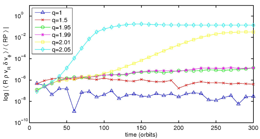
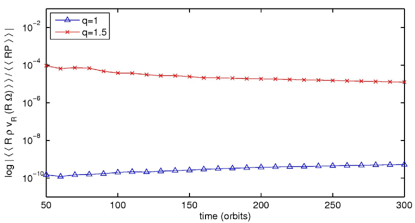
Refer to caption
Figure 3: Mean dimensionless angular momentum transport as a function of time in the Rayleigh rotational stability test for various values of q𝑞q.
Refer to caption
Figure 4: The cumulative mean (time- and space-average) of the dimensionless background radial angular momentum flux as a function of time for shear parameters q=1𝑞1q=1 and q=1.5𝑞1.5q=1.5 with unperturbed initial data.

10.3 Adiabatic Blast Wave

In this problem, we investigate a strong 2D shock using the HLLC solver. We use the parameter set of GS08 and compare the outputs of our cylindrical code with those from the Cartesian version of Athena. For the Cartesian version we use the domain (x,y)[0.5,0.5]×[0.75,0.75]𝑥𝑦0.50.50.750.75(x,y)\in[-0.5,0.5]\times[-0.75,0.75], and for the cylindrical version we use the domain (R,ϕ)[1,2]×[0.5,0.5]𝑅italic-ϕ120.50.5(R,\phi)\in[1,2]\times[-0.5,0.5] so that the physical domain spans an arc-length of Rmid(ϕmaxϕmin)=1.5subscript𝑅midsubscriptitalic-ϕmaxsubscriptitalic-ϕmin1.5R_{\text{mid}}(\phi_{\text{max}}-\phi_{\text{min}})=1.5 at Rmid=1.5subscript𝑅mid1.5R_{\text{mid}}=1.5, giving a roughly similar domain sizes. The initial conditions consist of a circular region of hot gas with radius R=0.1𝑅0.1R=0.1 and pressure P=10𝑃10P=10 in an ambient medium of uniform pressure P0=0.1subscript𝑃00.1P_{0}=0.1 and density ρ0=1subscript𝜌01\rho_{0}=1. We use a computational grid of 200×300200300200\times 300 cells, third-order reconstruction, and the HLLC fluxes with upwind-only integration for the L/R states in each version of the test. Contour plots of the density, pressure and specific kinetic energy densities of the evolved state at time t=0.2𝑡0.2t=0.2 are shown in Figure 5 using the cylindrical (left column) or Cartesian (right column) version of Athena. For additional comparison, 1D plots of these variables along a horizontal line through the center of the blast are shown in Figure 6, demonstrating excellent agreement between the Cartesian and cylindrical versions of Athena. Notice in the Cartesian version that symmetry is perfectly preserved by the integrator, which is most easily seen in the grid noise in the interior of the shell in Figure 5. Symmetry is also preserved rather well in the cylindrical version although in this case the grid is non-uniform.
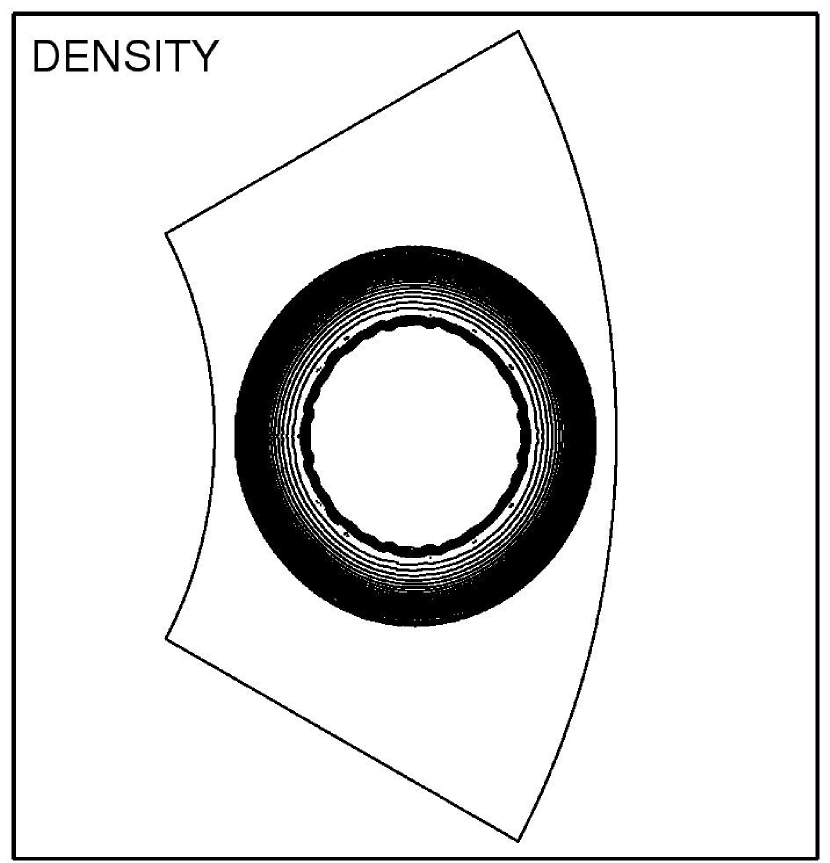
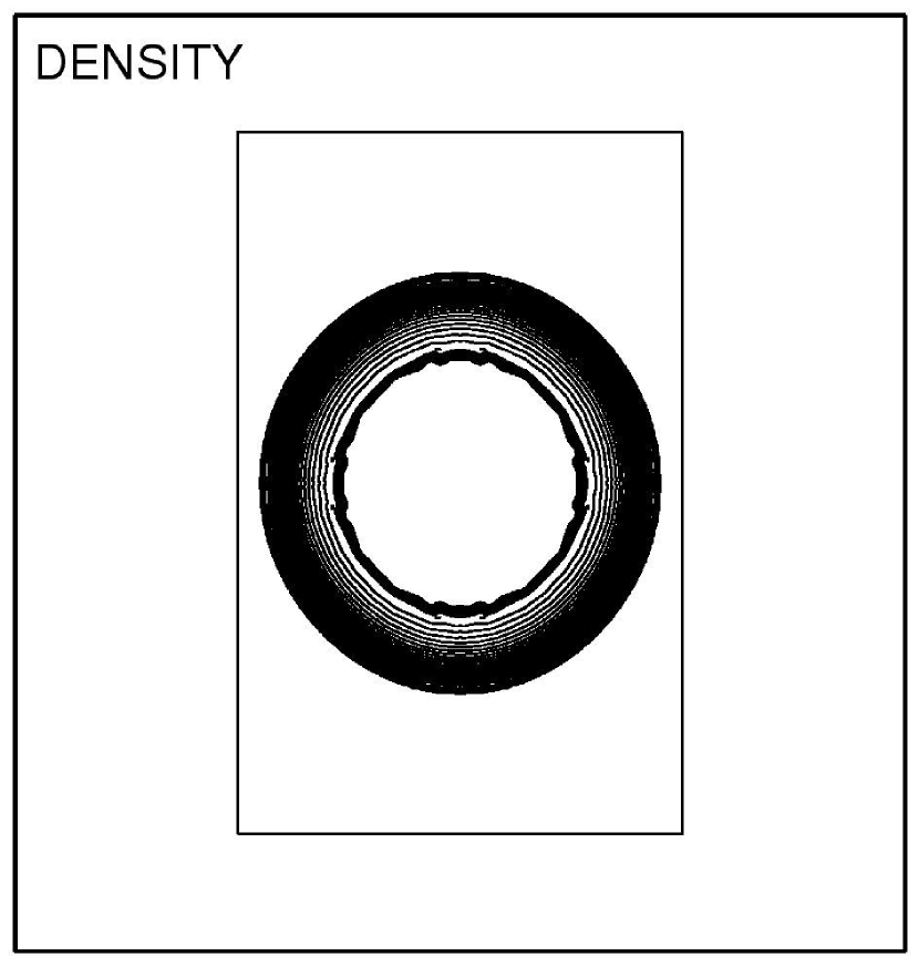
Refer to captionRefer to caption

Figure 5: Contours of selected variables of the evolved state (at time t=0.2𝑡0.2t=0.2) for the 2D hydrodynamic blast wave test using 200×300200300200\times 300 grid cells, third-order reconstruction, HLLC fluxes, and the cylindrical (left column) or Cartesian (right column) versions of Athena. Thirty equally spaced contours between the minimum and maximum are drawn in each plot.
Refer to caption
Refer to caption
Refer to caption
Figure 6: Plots of selected variables along a horizontal line through the center of the blast at time t=0.2𝑡0.2t=0.2 for the 2D hydrodynamic blast wave test (see Fig. 5 legend), using the cylindrical (circles) or Cartesian (solid line) versions of Athena.

10.4 Rotating Wind

In this problem, we investigate a steady, axisymmetric, rotating hydrodynamic wind as a test of angular momentum transport across a sonic transition. We adopt a Newtonian gravitational potential of the form Φg=GM/RsubscriptΦ𝑔𝐺𝑀𝑅\Phi_{g}=-GM/R. The constants of motion are given by

K𝐾\displaystyle K =Pργ,absent𝑃superscript𝜌𝛾\displaystyle=P\rho^{-\gamma}, (98)
M˙˙𝑀\displaystyle\dot{M} =RρvR,absent𝑅𝜌subscript𝑣𝑅\displaystyle=R\rho v_{R}, (99)
J𝐽\displaystyle J =Rvϕ.absent𝑅subscript𝑣italic-ϕ\displaystyle=Rv_{\phi}. (100)

This flow must satisfy the Bernoulli equation, =constantconstant\mathcal{B}={\rm constant}, along streamlines for

12v2+h+Φg,12superscript𝑣2subscriptΦ𝑔\mathcal{B}\equiv\text@frac{1}{2}v^{2}+h+\Phi_{g}, (101)

where

hdPρ=cs2γ1𝑑𝑃𝜌superscriptsubscript𝑐𝑠2𝛾1h\equiv\int\frac{dP}{\rho}=\frac{c_{s}^{2}}{\gamma-1} (102)

is the specific enthalpy of the gas.

We scale density and pressure to their values at infinity, ρρ()subscript𝜌𝜌\rho_{\infty}\equiv\rho(\infty) and PP()subscript𝑃𝑃P_{\infty}\equiv P(\infty), and the radial coordinate to some finite fiducial value, RBsubscript𝑅𝐵R_{B}. In terms of αρ/ρ𝛼𝜌subscript𝜌\alpha\equiv\rho/\rho_{\infty} and χR/RB𝜒𝑅subscript𝑅𝐵\chi\equiv R/R_{B}, the constant entropy parameter is K=c2/(γργ1)𝐾superscriptsubscript𝑐2𝛾superscriptsubscript𝜌𝛾1K=c_{\infty}^{2}/(\gamma\,\rho_{\infty}^{\gamma-1}), where c2γP/ρsuperscriptsubscript𝑐2𝛾subscript𝑃subscript𝜌c_{\infty}^{2}\equiv\gamma P_{\infty}/\rho_{\infty} is the square of the sound speed at infinity. At any radius, the local sound speed, radial velocity, and specific enthalpy satisfy

cs2superscriptsubscript𝑐𝑠2\displaystyle c_{s}^{2} =\displaystyle= c2αγ1,superscriptsubscript𝑐2superscript𝛼𝛾1\displaystyle c_{\infty}^{2}\alpha^{\gamma-1}, (103)
vR2superscriptsubscript𝑣𝑅2\displaystyle v_{R}^{2} =\displaystyle= R2c2αγ1,superscriptsubscript𝑅2superscriptsubscript𝑐2superscript𝛼𝛾1\displaystyle\mathcal{M}_{R}^{2}c_{\infty}^{2}\alpha^{\gamma-1}, (104)
h\displaystyle h =\displaystyle= 1γ1c2αγ1,1𝛾1superscriptsubscript𝑐2superscript𝛼𝛾1\displaystyle\frac{1}{\gamma-1}c_{\infty}^{2}\alpha^{\gamma-1}, (105)

where RvR/cssubscript𝑅subscript𝑣𝑅subscript𝑐𝑠\mathcal{M}_{R}\equiv v_{R}/c_{s} is the radial Mach number.

We define the dimensionless radial mass flux by

λM˙RBρc=χRα(γ+1)/2𝜆˙𝑀subscript𝑅𝐵subscript𝜌subscript𝑐𝜒subscript𝑅superscript𝛼𝛾12\lambda\equiv\frac{\dot{M}}{R_{B}\rho_{\infty}c_{\infty}}=\chi\mathcal{M}_{R}\alpha^{(\gamma+1)/2} (106)

and the dimensionless angular momentum by

ωJRBc=χvϕc.𝜔𝐽subscript𝑅𝐵subscript𝑐𝜒subscript𝑣italic-ϕsubscript𝑐\omega\equiv\frac{J}{R_{B}c_{\infty}}=\frac{\chi v_{\phi}}{c_{\infty}}. (107)

Solving equation (106) for α𝛼\alpha and introducing β2(γ1)/(γ+1)𝛽2𝛾1𝛾1\beta\equiv 2(\gamma-1)/(\gamma+1), we find that αγ1=[λ/(χR)]βsuperscript𝛼𝛾1superscriptdelimited-[]𝜆𝜒subscript𝑅𝛽\alpha^{\gamma-1}=[\lambda/(\chi\mathcal{M}_{R})]^{\beta}. Finally, taking RBsubscript𝑅𝐵R_{B} to be the Bondi radius, RBGM/c2subscript𝑅𝐵𝐺𝑀superscriptsubscript𝑐2R_{B}\equiv GM/c_{\infty}^{2}, we obtain the dimensionless Bernoulli equation

(12R2β+1γ1Rβ)λβ=[~γ1χβ+χβ1ω22χβ2],12superscriptsubscript𝑅2𝛽1𝛾1superscriptsubscript𝑅𝛽superscript𝜆𝛽delimited-[]~𝛾1superscript𝜒𝛽superscript𝜒𝛽1superscript𝜔22superscript𝜒𝛽2\left(\frac{1}{2}\mathcal{M}_{R}^{2-\beta}+\frac{1}{\gamma-1}\mathcal{M}_{R}^{-\beta}\right)\lambda^{\beta}=\left[\frac{\tilde{\mathcal{B}}}{\gamma-1}\chi^{\beta}+\chi^{\beta-1}-\frac{\omega^{2}}{2}\chi^{\beta-2}\right], (108)

where ~/h~subscript\tilde{\mathcal{B}}\equiv\mathcal{B}/h_{\infty} is the dimensionless Bernoulli constant, and hc2/(γ1)subscriptsuperscriptsubscript𝑐2𝛾1h_{\infty}\equiv c_{\infty}^{2}/(\gamma-1) is the specific enthalpy at infinity.

Figure 7 shows the contours of λ𝜆\lambda for various values of ω𝜔\omega, using an adiabatic index of γ=5/3𝛾53\gamma=5/3. For the ω=0𝜔0\omega=0 case, we recover a cylindrical version of Parker’s spherically symmetric wind (see, e.g., Spitzer, 1978). The bold lines represent the transonic solutions (wind and accretion) passing through the X-type saddle points. These solutions can be found by first writing equation (108) as (R)f(λ)=𝒢(χ)subscript𝑅𝑓𝜆𝒢𝜒\mathcal{F}(\mathcal{M}_{R})f(\lambda)=\mathcal{G}(\chi) and requiring that =𝒢=0superscriptsuperscript𝒢0\mathcal{F}^{\prime}=\mathcal{G}^{\prime}=0. The first constraint implies that R=1subscript𝑅1\mathcal{M}_{R}=1, i.e. the saddle point is the sonic point. The second constraint yields a quadratic in χ𝜒\chi, and for ω(0,ωmax)𝜔0subscript𝜔max\omega\in(0,\omega_{\rm max}), there are two distinct, positive solutions,

χ±=3γ±(3γ)216~ω24~,subscript𝜒plus-or-minusplus-or-minus3𝛾superscript3𝛾216~superscript𝜔24~\chi_{\pm}=\frac{3-\gamma\pm\sqrt{(3-\gamma)^{2}-16\tilde{\mathcal{B}}\omega^{2}}}{4\tilde{\mathcal{B}}}, (109)

where ωmax(3γ)/(4~1/2)subscript𝜔max3𝛾4superscript~12\omega_{\rm max}\equiv(3-\gamma)/(4\tilde{\mathcal{B}}^{1/2}). It can be shown that χsubscript𝜒\chi_{-} gives an O-type critical point and χ+subscript𝜒\chi_{+} gives the desired transonic critical point. For ω>ωmax𝜔subscript𝜔max\omega>\omega_{\rm max}, no transonic solutions exist. Note further that no transonic solutions exist for χ<χmin𝜒subscript𝜒min\chi<\chi_{\rm min}, where χminsubscript𝜒min\chi_{\rm min} represents the point at which the transonic wind solution for which Rsubscript𝑅\mathcal{M}_{R}\to\infty as χ𝜒\chi\to\infty joins the transonic accretion solution for which R0subscript𝑅0\mathcal{M}_{R}\to 0 as χ𝜒\chi\to\infty (see, e.g., the lower-left panel of Figure 7). We define χminsubscript𝜒min\chi_{\rm min} to be the smallest value of χ0𝜒0\chi\geq 0 for which 𝒢(χ)0𝒢𝜒0\mathcal{G}(\chi)\geq 0, which is given by

χmin=(γ1)+(γ1)2+2~ω22~.subscript𝜒min𝛾1superscript𝛾122~superscript𝜔22~\chi_{\rm min}=\frac{-(\gamma-1)+\sqrt{(\gamma-1)^{2}+2\tilde{\mathcal{B}}\omega^{2}}}{2\tilde{\mathcal{B}}}. (110)

Finally, the critical value of the radial mass flux, λcsubscript𝜆c\lambda_{\rm c}, is defined by equation (108) with χ=χ+𝜒subscript𝜒\chi=\chi_{+} and R=1subscript𝑅1\mathcal{M}_{R}=1, which is given by

λc=[χ+β2(χ+ω2)]1/β.subscript𝜆csuperscriptdelimited-[]superscriptsubscript𝜒𝛽2subscript𝜒superscript𝜔21𝛽\lambda_{\rm c}=\left[\chi_{+}^{\beta-2}(\chi_{+}-\omega^{2})\right]^{1/\beta}. (111)

For our code test, we use γ=5/3𝛾53\gamma=5/3 (i.e. β=1/2𝛽12\beta=1/2), ω=0.3𝜔0.3\omega=0.3, and ~=1~1\tilde{\mathcal{B}}=1, which give the transonic solution shown in Figure 7c. The critical point occurs at χ+0.479subscript𝜒0.479\chi_{+}\approx 0.479, with λc1.377subscript𝜆𝑐1.377\lambda_{c}\approx 1.377. We solve the problem on the domain χ[χ,2]𝜒subscript𝜒2\chi\in[\chi_{-},2], where χ0.188subscript𝜒0.188\chi_{-}\approx 0.188, using bisection with a tolerance of ϵ=1010italic-ϵsuperscript1010\epsilon=10^{-10} to evaluate Rsubscript𝑅\mathcal{M}_{R} at each χ𝜒\chi from equation (108). Once Rsubscript𝑅\mathcal{M}_{R} is known, vRsubscript𝑣𝑅v_{R}, ρ𝜌\rho, and P𝑃P follow algebraically. We choose units such that GM=c=1𝐺𝑀subscript𝑐1GM=c_{\infty}=1, which yields RB=1subscript𝑅𝐵1R_{B}=1. We fix the solution at the inner and outer boundaries and evolve the initial solution long enough for it to settle into equilibrium.

Figure 8 shows the convergence of the L2subscript𝐿2L_{2} norm of the L1subscript𝐿1L_{1} error vector for the solution at time t=5.0𝑡5.0t=5.0. These data were computed using the Roe fluxes, second-order reconstruction, and the 1D; the results were similar for all combinations of Roe or HLLC fluxes and second- or third-order reconstruction. The test was also performed using the 2D and 3D integrator with a few grid cells in the transverse directions.

This test clearly demonstrates the code’s ability to maintain smooth, steady hydrodynamic flows in both subsonic and supersonic regimes, as well as its ability to conserve angular momentum to second-order in cylindrical geometry.
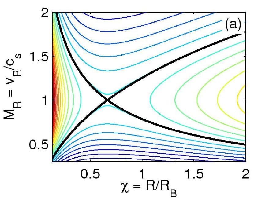
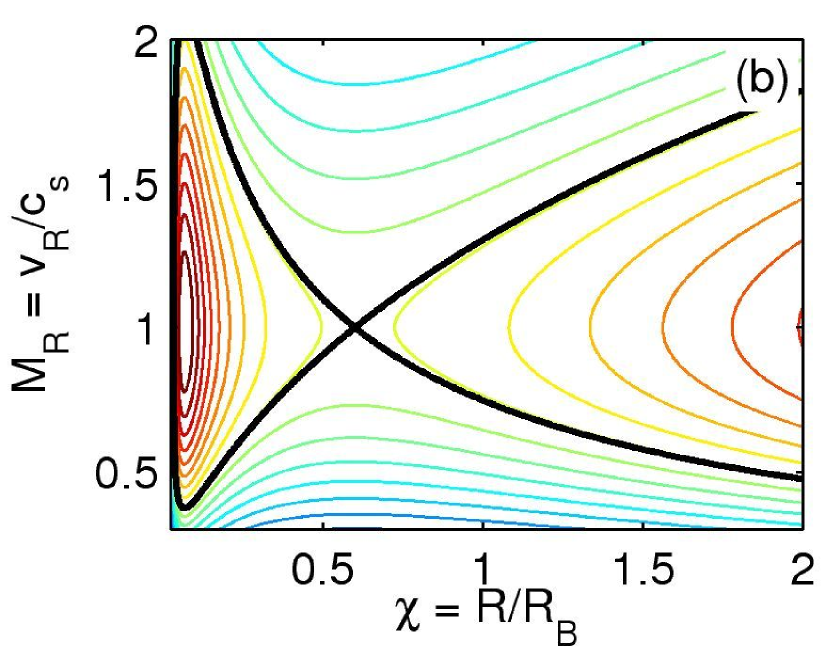
Refer to captionRefer to caption

Figure 7: Contours of the dimensionless mass flux, λ𝜆\lambda, for a rotating hydrodynamic steady flow with γ=5/3𝛾53\gamma=5/3 and dimensionless Bernoulli constant ~=1~1\tilde{\mathcal{B}}=1. The scaled angular momentum in each panel is (a) ω=0𝜔0\omega=0, (b) ω=0.2𝜔0.2\omega=0.2, (c) ω=0.3𝜔0.3\omega=0.3, and (d) ω=1/3𝜔13\omega=1/3. The critical transonic contours are shown in bold.
Refer to caption
Figure 8: Convergence of the RMS error in the L1subscript𝐿1L_{1}-norm for various levels of discretization of the rotating hydrodynamic wind test in 1D, 2D and 3D. For reference, we have plotted a line of slope 22-2 (dashed) to show that the convergence is second-order in 1/N1𝑁1/N.

10.5 Field Loop Advection

In this problem, we investigate the advection of a weak field loop in 2D and 3D cylindrical coordinates, analogous to the Cartesian test appearing in \al@gar05,gar08; \al@gar05,gar08. The main difference with our test is that we advect the field loop in the ϕitalic-ϕ\phi-direction only as opposed to a more general advection oblique to the grid. We use the computational domain (R,ϕ)[1,2]×[2/3,2/3]𝑅italic-ϕ122323(R,\phi)\in[1,2]\times[-2/3,2/3], which has the same total area as the Cartesian version of the test. We use periodic boundary conditions in ϕitalic-ϕ\phi and fixed boundary conditions in R𝑅R. We use uniform initial density ρ0=1subscript𝜌01\rho_{0}=1 and pressure P0=1subscript𝑃01P_{0}=1 with a solid-body rotation profile of vϕ=Ω0Rsubscript𝑣italic-ϕsubscriptΩ0𝑅v_{\phi}=\Omega_{0}R, where we set Ω0=4/3subscriptΩ043\Omega_{0}=4/3 so that the field loop is advected once across the grid by t=1𝑡1t=1. The initial z𝑧z-component of the magnetic field is 00, and the R𝑅R- and ϕitalic-ϕ\phi-components are set using the z𝑧z-component of the magnetic vector potential

Az{A0(a0r)for ra0,0for r>a0,subscript𝐴𝑧casessubscript𝐴0subscript𝑎0𝑟for 𝑟subscript𝑎00for 𝑟subscript𝑎0A_{z}\equiv\left\{\begin{array}[]{ll}A_{0}(a_{0}-r)&\text{for }r\leq a_{0},\\ 0&\text{for }r>a_{0}\end{array}\right., (112)

where a0subscript𝑎0a_{0} is the radius of the field loop and rR2+R022RR0cos(ϕϕ0)𝑟superscript𝑅2superscriptsubscript𝑅022𝑅subscript𝑅0italic-ϕsubscriptitalic-ϕ0r\equiv\sqrt{R^{2}+R_{0}^{2}-2RR_{0}\cos(\phi-\phi_{0})} is the distance from the center of the loop (R0,ϕ0)subscript𝑅0subscriptitalic-ϕ0(R_{0},\phi_{0}). We use A0=103subscript𝐴0superscript103A_{0}=10^{-3} and a0=0.3subscript𝑎00.3a_{0}=0.3 so that inside the field loop P/B=106𝑃𝐵superscript106P/B=10^{6} and the field loop should be advected passively.

Figure 9 shows the magnetic energy density B2/2superscript𝐵22B^{2}/2 and magnetic field lines at times t=0𝑡0t=0 and t=2𝑡2t=2 for the 2D problem. The field lines are the contours of Azsubscript𝐴𝑧A_{z} which can be readily computed since the field is planar and the CTU+CT algorithm preserves the 𝑩=0𝑩0\nabla\cdot\boldsymbol{B}=0 condition. Note that the circular shape of the field lines is nicely preserved.

Figure 10 shows the time evolution of the volume-averaged magnetic energy density. The dissipation is well-described by a power law of the form B2/2=A(1(t/τ)α)delimited-⟨⟩superscript𝐵22𝐴1superscript𝑡𝜏𝛼\langle B^{2}/2\rangle=A(1-(t/\tau)^{\alpha}) (for tτmuch-less-than𝑡𝜏t\ll\tau), with A=7.02×10⁸𝐴7.02superscript108A=7.02\times 10^{-8}, τ=1.46×10⁴𝜏1.46superscript104\tau=1.46\times 10^{4}, and α=0.342𝛼0.342\alpha=0.342, and with a residual error of 0.05800.05800.0580. Note that the overall dissipation in this problem is less than that of the Cartesian version since the advection is only in one direction; GS05 found τ=1.06×10⁴𝜏1.06superscript104\tau=1.06\times 10^{4} and α=0.291𝛼0.291\alpha=0.291 for a similar fit.

Refer to captionRefer to caption

Figure 9: For the 2D field loop advection test, we show the magnetic energy density B2/2superscript𝐵22B^{2}/2 at times t=0𝑡0t=0 and t=2𝑡2t=2 in panels (a) and (b), respectively. Panels (c) and (d) contain magnetic field lines at t=0𝑡0t=0 and t=2𝑡2t=2, respectively.
Refer to caption
Figure 10: Time evolution showing dissipation of the volume-averaged magnetic energy density B2/2superscript𝐵22B^{2}/2 for the 2D field loop advection test. The solid line represents a power law fit (for tτmuch-less-than𝑡𝜏t\ll\tau) to the data points with residual 0.05800.05800.0580.

10.6 Blast Wave in a Strong Magnetic Field

In this problem, we investigate 2D and 3D MHD shocks in a strongly magnetized medium with low plasma-β𝛽\beta, denoted βp2P/Bsubscript𝛽𝑝2𝑃𝐵\beta_{p}\equiv 2P/B. We run two problems, one with B0=1subscript𝐵01B_{0}=1 and βp=0.2subscript𝛽𝑝0.2\beta_{p}=0.2 using the parameter set of GS08, and another with B0=10subscript𝐵010B_{0}=10 and βp=0.02subscript𝛽𝑝0.02\beta_{p}=0.02 using the parameter set of Londrillo & Del Zanna (2000). In each case, we compare the outputs of the cylindrical and Cartesian versions of Athena.

The moderate B𝐵B-field, βp=0.2subscript𝛽𝑝0.2\beta_{p}=0.2 case uses HLLD fluxes and the same setup as the hydrodynamic blast described in §10.3, but with a uniform background magnetic field of strength B0=1subscript𝐵01B_{0}=1 oriented at a 45superscript4545^{\circ} angle to the positive x^^𝑥\hat{x}- or R^^𝑅\hat{R}-axis. For the 2D case, contour plots of the density, pressure, specific kinetic energy, and magnetic energy are shown in Figure 11 based on the cylindrical (left column) or Cartesian (right column) versions of Athena. Figure 12 shows a plot of these variables along a horizontal line through the center of the blast. Note that in the Cartesian version, the background field is uniformly inclined to the grid, but in the cylindrical version, the angle the background field makes with the grid changes as a function of ϕitalic-ϕ\phi; nonetheless, a high degree of symmetry is observed in the solution. We have also tested a 3D analogue of this problem on a 2003superscript2003200^{3} grid with z[0.5,0.5]𝑧0.50.5z\in[-0.5,0.5]. Again, plots of selected variables along a horizontal line through the center of the blast (in the z=0𝑧0z=0 plane) in Figure 13 show agreement between the Cartesian and cylindrical versions of Athena.

The strong B𝐵B-field, βp=0.02subscript𝛽𝑝0.02\beta_{p}=0.02 case uses the domain (x,y)[0.5,0.5]×[0.5,0.5]𝑥𝑦0.50.50.50.5(x,y)\in[-0.5,0.5]\times[-0.5,0.5] for the Cartesian version, and for the cylindrical version, uses the domain (R,ϕ)[1,2]×[2/3,2/3]𝑅italic-ϕ122323(R,\phi)\in[1,2]\times[2/3,2/3], giving a roughly similar domain size in each case. The initial conditions consist of a circular region of hot gas with radius R0=0.125subscript𝑅00.125R_{0}=0.125 and pressure P=100𝑃100P=100 in an ambient medium of uniform pressure P0=1subscript𝑃01P_{0}=1 and density ρ0=1subscript𝜌01\rho_{0}=1. There is uniform background magnetic field of strength B0=10subscript𝐵010B_{0}=10 oriented parallel to the x𝑥x-axis. We use a computational grid of 2002superscript2002200^{2} cells, third-order reconstruction and the HLLD fluxes with upwind-only integration for the L/R states. The density, pressure, specific kinetic energy, and magnetic energy along a horizontal line through the center of the blast at time t=0.02𝑡0.02t=0.02 are shown in Figure 14, with comparison to the Cartesian version of Athena. We have also conducted a 3D analogue of this test on a 2003superscript2003200^{3} grid with z[0.5,0.5]𝑧0.50.5z\in[-0.5,0.5]. Figure 15 shows a comparison of contour plots with the Cartesian version of Athena, and Figure 16 shows a comparison along a horizontal line through the center of the blast (in the z=0𝑧0z=0 plane).
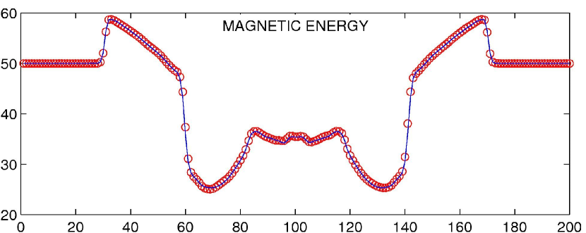
Refer to captionRefer to caption

Figure 11: Contours of selected variables of the evolved state (at time t=0.2𝑡0.2t=0.2) for the 2D MHD blast wave test with B0=1subscript𝐵01B_{0}=1 and βp=0.2subscript𝛽𝑝0.2\beta_{p}=0.2 using 200×300200300200\times 300 grid cells, third-order reconstruction, HLLD fluxes, and using the cylindrical (left column) or Cartesian (right column) versions of Athena. Thirty equally spaced contours between the minimum and maximum are drawn in each plot.
Refer to caption
Refer to caption
Refer to caption
Refer to caption
Figure 12: Plots of selected variables along a horizontal line through the center of the blast at time t=0.2𝑡0.2t=0.2 for the 2D MHD blast wave test with B0=1subscript𝐵01B_{0}=1 and βp=0.2subscript𝛽𝑝0.2\beta_{p}=0.2 using the cylindrical (circles) or Cartesian (solid line) versions of Athena.
Refer to caption
Refer to caption
Refer to caption
Refer to caption
Figure 13: Plots of selected variables along a horizontal line through the center of the blast at time t=0.2𝑡0.2t=0.2 for the 3D MHD blast wave test with B0=1subscript𝐵01B_{0}=1 and βp=0.2subscript𝛽𝑝0.2\beta_{p}=0.2 using the cylindrical (circles) or Cartesian (solid line) versions of Athena.
Refer to caption
Refer to caption
Refer to caption
Refer to caption
Figure 14: Plots of selected variables along a horizontal line through the center of the blast at time t=0.02𝑡0.02t=0.02 for the 2D MHD blast wave test with B0=10subscript𝐵010B_{0}=10 and βp=0.02subscript𝛽𝑝0.02\beta_{p}=0.02 using the cylindrical (circles) or Cartesian (solid line) versions of Athena.

Refer to captionRefer to caption

Figure 15: Contours of selected variables at time t=0.02𝑡0.02t=0.02 for the 3D MHD blast wave test with B0=10subscript𝐵010B_{0}=10 and βp=0.02subscript𝛽𝑝0.02\beta_{p}=0.02 using 2003superscript2003200^{3} grid cells and the cylindrical (top row) or Cartesian (bottom row) versions of Athena. Thirty equally spaced contours between the minimum and maximum are drawn in each plot.
Refer to caption
Refer to caption
Refer to caption
Refer to caption
Figure 16: Plots of selected variables along a horizontal line through the center of the blast at time t=0.02𝑡0.02t=0.02 for the 3D MHD blast wave test with B0=10subscript𝐵010B_{0}=10 and βp=0.02subscript𝛽𝑝0.02\beta_{p}=0.02 using the cylindrical (circles) or Cartesian (solid line) versions of Athena.

10.7 Weber-Davis Wind

In this problem, we investigate a cylindrical version of the Weber-Davis wind solution as described in Sakurai (1985). We assume a steady, axisymmetric, 2D MHD flow with planar magnetic field, and a gravitational potential Φg=GM/RsubscriptΦ𝑔𝐺𝑀𝑅\Phi_{g}=-GM/R. The constants of motion are K=Pργ𝐾𝑃superscript𝜌𝛾K=P\rho^{-\gamma}, M˙=RρvR˙𝑀𝑅𝜌subscript𝑣𝑅\dot{M}=R\rho v_{R}, f=RBR𝑓𝑅subscript𝐵𝑅f=RB_{R}, β=BR/(ρvR)𝛽subscript𝐵𝑅𝜌subscript𝑣𝑅\beta=B_{R}/(\rho v_{R}), as well as

ΩΩ\displaystyle\Omega =\displaystyle= 1R(vϕBϕβρ),1𝑅subscript𝑣italic-ϕsubscript𝐵italic-ϕ𝛽𝜌\displaystyle\text@frac{1}{R}\left(v_{\phi}-\frac{B_{\phi}}{\beta\rho}\right), (113a)
J𝐽\displaystyle J =\displaystyle= R(vϕβBϕ)=R2Ω+Ruϕ(1β2ρ),𝑅subscript𝑣italic-ϕ𝛽subscript𝐵italic-ϕsuperscript𝑅2Ω𝑅subscript𝑢italic-ϕ1superscript𝛽2𝜌\displaystyle R(v_{\phi}-\beta B_{\phi})=R^{2}\Omega+Ru_{\phi}(1-\beta^{2}\rho), (113b)
\displaystyle\mathcal{B} =\displaystyle= ½(uR2+uϕ2)+h+Φg12(ΩR)2.½superscriptsubscript𝑢𝑅2superscriptsubscript𝑢italic-ϕ2subscriptΦ𝑔12superscriptΩ𝑅2\displaystyle\text@onehalf(u_{R}^{2}+u_{\phi}^{2})+h+\Phi_{g}-\text@frac{1}{2}(\Omega R)^{2}. (113c)

Here, 𝒖(vR,vϕRΩ, 0)𝒖subscript𝑣𝑅subscript𝑣italic-ϕ𝑅Ω 0\boldsymbol{u}\equiv(v_{R},\,v_{\phi}-R\Omega,\,0) is the velocity in a frame rotating at angular velocity ΩΩ\Omega, and in this frame 𝑩=βρ𝒖𝑩𝛽𝜌𝒖\boldsymbol{B}=\beta\rho\boldsymbol{u}, so that the fluid feels no force from the magnetic field. Note that the Bernoulli parameter in the rotating frame includes a centrifugal potential contribution. The Alfvén Mach number in the rotating frame is given by Au/cA=1/β2ρsubscript𝐴𝑢subscript𝑐𝐴1superscript𝛽2𝜌\mathcal{M}_{A}\equiv u/c_{A}=1/\sqrt{\beta^{2}\rho}. Let RAsubscript𝑅𝐴R_{A} and ρAsubscript𝜌𝐴\rho_{A} denote the radius and density, respectively, at the Alfvén Mach point, i.e. where A=1subscript𝐴1\mathcal{M}_{A}=1. Then β=1/ρA𝛽1subscript𝜌𝐴\beta=1/\sqrt{\rho_{A}} and J=RA2Ω𝐽superscriptsubscript𝑅𝐴2ΩJ=R_{A}^{2}\Omega.

Letting xR/RA𝑥𝑅subscript𝑅𝐴x\equiv R/R_{A} and yρ/ρA=ρβ2=A2𝑦𝜌subscript𝜌𝐴𝜌superscript𝛽2superscriptsubscript𝐴2y\equiv\rho/\rho_{A}=\rho\beta^{2}=\mathcal{M}_{A}^{-2} denote the scaled radius and density, respectively, the Bernoulli parameter is

=GMRA[η2x2y2+ω2((1/xx1y)2x2)+θγ1yγ11x],𝐺𝑀subscript𝑅𝐴delimited-[]𝜂2superscript𝑥2superscript𝑦2𝜔2superscript1𝑥𝑥1𝑦2superscript𝑥2𝜃𝛾1superscript𝑦𝛾11𝑥\mathcal{B}=\frac{GM}{R_{A}}\left[\frac{\eta}{2x^{2}y^{2}}+\frac{\omega}{2}\left(\left(\frac{1/x-x}{1-y}\right)^{2}-x^{2}\right)+\frac{\theta}{\gamma-1}y^{\gamma-1}-\frac{1}{x}\right], (114)

where we have defined the scaled parameters

η𝜂\displaystyle\eta \displaystyle\equiv M˙2RAρA2GM,superscript˙𝑀2subscript𝑅𝐴superscriptsubscript𝜌𝐴2𝐺𝑀\displaystyle\frac{\dot{M}^{2}}{R_{A}\rho_{A}^{2}GM}, (115a)
θ𝜃\displaystyle\theta \displaystyle\equiv γKρAγ1RAGM,𝛾𝐾superscriptsubscript𝜌𝐴𝛾1subscript𝑅𝐴𝐺𝑀\displaystyle\frac{\gamma K\rho_{A}^{\gamma-1}R_{A}}{GM}, (115b)
ω𝜔\displaystyle\omega \displaystyle\equiv RA3Ω2GM.superscriptsubscript𝑅𝐴3superscriptΩ2𝐺𝑀\displaystyle\frac{R_{A}^{3}\Omega^{2}}{GM}. (115c)

Letting ~/(GM/RA)~𝐺𝑀subscript𝑅𝐴\tilde{\mathcal{B}}\equiv\mathcal{B}/(GM/R_{A}), we have

x~x𝑥~𝑥\displaystyle x\frac{\partial\tilde{\mathcal{B}}}{\partial x} =\displaystyle= ηx2y2+ω((x21/x2)(1y)2x2)+1x,𝜂superscript𝑥2superscript𝑦2𝜔superscript𝑥21superscript𝑥2superscript1𝑦2superscript𝑥21𝑥\displaystyle-\frac{\eta}{x^{2}y^{2}}+\omega\left(\frac{(x^{2}-1/x^{2})}{(1-y)^{2}}-x^{2}\right)+\frac{1}{x}, (116a)
y~y𝑦~𝑦\displaystyle y\frac{\partial\tilde{\mathcal{B}}}{\partial y} =\displaystyle= ηx2y2+ωy(1/xx)2(1y)3+θyγ1.𝜂superscript𝑥2superscript𝑦2𝜔𝑦superscript1𝑥𝑥2superscript1𝑦3𝜃superscript𝑦𝛾1\displaystyle-\frac{\eta}{x^{2}y^{2}}+\omega y\frac{(1/x-x)^{2}}{(1-y)^{3}}+\theta y^{\gamma-1}. (116b)

To find wind solutions, we solve the Bernoulli equation (114) under the constraint that the solution be locally flat at the slow- and fast-magnetosonic points, i.e. ~/x=~/y=0~𝑥~𝑦0\partial\tilde{\mathcal{B}}/\partial x=\partial\tilde{\mathcal{B}}/\partial y=0 at (xs,ys)subscript𝑥𝑠subscript𝑦𝑠(x_{s},\,y_{s}) and (xf,yf)subscript𝑥𝑓subscript𝑦𝑓(x_{f},\,y_{f}). We will specify θ𝜃\theta and ω𝜔\omega, and let η𝜂\eta, ~~\tilde{\mathcal{B}}, xssubscript𝑥𝑠x_{s}, yssubscript𝑦𝑠y_{s}, xfsubscript𝑥𝑓x_{f}, and yfsubscript𝑦𝑓y_{f} vary. Note that this becomes a system of six equations in six unknowns, so if a solution exists, it must be unique. Following Sakurai (1985), we use the parameters γ=1.2𝛾1.2\gamma=1.2, θ=1.5𝜃1.5\theta=1.5 and ω=0.3𝜔0.3\omega=0.3 as for the spherically symmetric solar wind model of Weber and Davis. The numerical solution is given in Table 1.

We solve the problem on the domain x[0.4,1.8]𝑥0.41.8x\in[0.4,1.8], so that the wind solution passes through all three critical points. We choose units such that GM=1𝐺𝑀1GM=1 and fix the initial solution at the inner- and outer-boundaries, evolving it long enough for equilibrium to develop. Figure 17 shows the convergence of the RMS error in the L1subscript𝐿1L_{1}-norm of the solution at t=5.0𝑡5.0t=5.0 compared to the initial solution. These data were computed using the Roe fluxes, second-order reconstruction, and the 1D integrator; the results were similar for all combinations of Roe/HLLD fluxes and second-/third-order reconstruction. Because the 2D and 3D algorithms differ significantly from the 1D version, especially in their treatment of magnetic fields, we present the results of the same test using these integrators on grids which are essentially one-dimensional, but contain a few grid cells in each transverse direction considered.

Evidently, the algorithm yields second-order convergence for smooth MHD flows, and is able to maintain a steady magnetized solution, also conserving angular momentum as it is exchanged between the fluid and magnetic field.
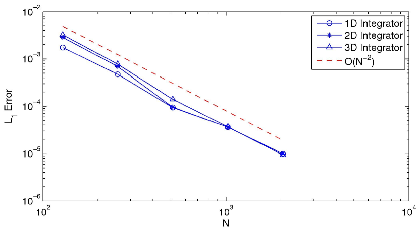
Refer to caption
Figure 17: Convergence of the RMS error in the L1subscript𝐿1L_{1}-norm for various levels of discretization of the Weber-Davis MHD wind test in 1D, 2D and 3D. For reference, we have plotted a line of slope 22-2 (dashed) to show that the convergence is second-order in 1/N1𝑁1/N.

11 Conclusion

We have described an adaptation of the Athena astrophysical MHD code for cylindrical coordinates. The original Cartesian code uses a combination of higher-order Godunov methods (based on the CTU algorithm of Colella) to evolve the mass-density, momenta, and total energy, and constrained transport (Evans & Hawley, 1988) to evolve the magnetic fields. We have described modifications to the second- and third-order reconstruction schemes, the finite-volume and finite-area formulations of the MHD equations, and the inclusion of geometric source terms.

Our approach is advantageous in that it does not require modification to the majority of the existing code, in particular to the Riemann solvers and eigensystems. Furthermore, our approach to implementing cylindrical coordinates could be applied in a straightforward manner to enable other curvilinear coordinate systems, such as spherical coordinates, in the Athena code as well as other higher-order Godunov codes.

Finally, our code and test suite are publicly available for download on the Web. The code is currently being used for a variety of applications, including studies of global accretion disks, and we hope it will be of use to many others studying problems in astrophysical fluid dynamics.

The authors would like to thank Jim Stone for helpful discussions about the Athena algorithms, and Peter Teuben for his assistance with the code package. This work was supported by grant AST 0507315 from the National Science Foundation.

References

  • Blondin & Lufkin (1993) Blondin, J. M., & Lufkin, E. A. 1993, ApJS, 88, 589
  • Colella (1990) Colella, P. 1990, J. Comp. Phys., 87, 171
  • Colella & Sekora (2008) Colella, P., & Sekora, M. D. 2008, J. Comp. Phys., 227, 7069
  • Colella & Woodward (1984) Colella, P., & Woodward, P. R. 1984, J. Comp. Phys., 54, 174
  • Einfeldt et al. (1991) Einfeldt, B., Roe, P. L., Munz, C. D., & Sjogreen, B. 1991, J. Comp. Phys., 92, 273
  • Evans & Hawley (1988) Evans, C. R., & Hawley, J. F. 1988, ApJ, 332, 659
  • Fryxell et al. (2000) Fryxell, B., et al. 2000, ApJS, 131, 273
  • Gardiner & Stone (2005) Gardiner, T. A., & Stone, J. M. 2005, J. Comp. Phys., 205, 509
  • Gardiner & Stone (2008) —. 2008, J. Comp. Phys., 227, 4123
  • Harten et al. (1983) Harten, A., Lax, P. D., & van Leer, B. 1983, SIAM Review, 25, 35
  • Ji et al. (2006) Ji, H., Burin, M., Schartman, E., & Goodman, J. 2006, Nature, 444, 343
  • Leveque (2002) Leveque, R. J. 2002, Finite Volume Methods For Hyperbolic Problems (Cambridge: Cambridge University Press)
  • Londrillo & Del Zanna (2000) Londrillo, P., & Del Zanna, L. 2000, ApJ, 530, 508
  • Mignone et al. (2007) Mignone, A., Bodo, G., Massaglia, S., Matsakos, T., Tesileanu, O., Zanni, C., & Ferrari, A. 2007, ApJS, 170, 228
  • Mihalas & Mihalas (1984) Mihalas, D., & Mihalas, B. W. 1984, Foundations of radiation hydrodynamics (New York, Oxford University Press, 1984, 731 p.)
  • Miyoshi & Kusano (2005) Miyoshi, T., & Kusano, K. 2005, Journal of Computational Physics, 208, 315
  • Powell et al. (1999) Powell, K. G., Roe, P. L., Linde, T. J., Gombosi, T. I., & de Zeeuw, D. L. 1999, J. Comp. Phys., 154, 284
  • Roe (1981) Roe, P. L. 1981, Journal of Computational Physics, 43, 357
  • Sakurai (1985) Sakurai, T. 1985, A&A, 152, 121
  • Spitzer (1978) Spitzer, L. 1978, Physical processes in the interstellar medium, ed. L. Spitzer
  • Stone et al. (2008) Stone, J. M., Gardiner, T. A., Teuben, P., Hawley, J. F., & Simon, J. B. 2008, ArXiv e-prints, 804
  • Stone & Norman (1992a) Stone, J. M., & Norman, M. L. 1992a, ApJS, 80, 753
  • Stone & Norman (1992b) —. 1992b, ApJS, 80, 791
  • Teyssier (2002) Teyssier, R. 2002, A&A, 385, 337
  • Toro (1999) Toro, E. 1999, Riemann Solvers and Numerical Methods for Fluid Dynamics: A Practical Introduction
  • Tóth (1996) Tóth, G. 1996, Astrophysical Letters Communications, 34, 245
  • Ziegler (2004) Ziegler, U. 2004, J. Comp. Phys., 196, 393
Table 1: Weber-Davis Wind Parameters
Parameter Value
γ𝛾\gamma 1.21.21.2
θ𝜃\theta 1.51.51.5
ω𝜔\omega 0.30.30.3
η𝜂\eta 2.36092.36092.3609
~~\tilde{\mathcal{B}} 7.87457.87457.8745
xssubscript𝑥𝑠x_{s} 0.52430.52430.5243
yssubscript𝑦𝑠y_{s} 2.49862.49862.4986
xfsubscript𝑥𝑓x_{f} 1.63831.63831.6383
yfsubscript𝑦𝑓y_{f} 0.53740.53740.5374