Ammann Tilings in Symplectic Geometry

Ammann Tilings in Symplectic Geometry

Fiammetta BATTAGLIA ^† and Elisa PRATO ^‡ F. Battaglia and E. Prato

^† Dipartimento di Matematica e Informatica “U. Dini”, Via S. Marta 3, 50139 Firenze, Italy fiammetta.battaglia@unifi.it http://www.dma.unifi.it/~fiamma/

^‡ Dipartimento di Matematica e Informatica “U. Dini”, Piazza Ghiberti 27, 50122 Firenze, Italy elisa.prato@unifi.it http://www.math.unifi.it/people/eprato/

Received November 09, 2012, in final form February 27, 2013; Published online March 06, 2013

In this article we study Ammann tilings from the perspective of symplectic geometry. Ammann tilings are nonperiodic tilings that are related to quasicrystals with icosahedral symmetry. We associate to each Ammann tiling two explicitly constructed highly singular symplectic spaces and we show that they are diffeomorphic but not symplectomorphic. These spaces inherit from the tiling its very interesting symmetries.

symplectic quasifold; nonperiodic tiling; quasilattice

53D20; 52C23

1 Introduction

Our general aim is to study the connection between symplectic geometry and the nonperiodic tilings that are related to the geometry of quasicrystals. Considering these tilings from the symplectic viewpoint provides a concrete way of obtaining new examples of highly singular symplectic spaces that are endowed with very rich symmetries. These examples effectively contribute to understanding the theoretical aspects of the geometry of this type of singular spaces. Moreover, we expect that symplectic geometry may be used to shed light on the study of the tilings.

We started this program with the study of two tilings of the plane: Penrose rhombus [2] and kite and dart [3] tilings.

In this article we focus our attention for the first time on three-dimensional tilings. We consider Ammann tilings, which are the three-dimensional analogues of Penrose rhombus tilings. They were introduced by Ammann in the 70’s [10] and turned out to be related to quasicrystals with icosahedral symmetry [6]. As we will see later, the third dimension yields an initially unexpected richness and complexity.

The main idea underlying the connection between symplectic geometry and tilings is a generalization [8] of the Delzant construction [5], which we use to associate to each tile an explicitly constructed symplectic space. We recall that the Delzant construction associates a symplectic toric $2n$-manifold to each simple convex polytope in $\big{(}\mbox{\bbb{R}}^{n}\big{)}^{*}$, which is rational with respect to a lattice and satisfies an additional integrality condition. The problem, in the setting of nonperiodic tilings related to quasicrystals, is that either the tiles are not individually rational, or they are not simultaneously rational with respect to the same lattice. In the generalized construction, however, the lattice is replaced by a quasilattice and rationality is replaced by the notion of quasirationality. The resulting space is a $2n$-dimensional quasifold, a generalization of manifolds and orbifolds that was first introduced by the second-named author in [8]; the group acting is no longer a torus but a quasitorus [8].

Ammann tilings are made of two kinds of tiles: an oblate rhombohedron and a prolate rhombohedron having same edge lengths. These rhombohedra, although separately rational, are not simultaneously rational with respect to the same lattice. However, the geometry of the tiling ensures that it is possible to choose a quasilattice $F$ having the property that each rhombohedron of the tiling is quasirational with respect to $F$ (Proposition 3.1). We then apply the generalized Delzant construction simultaneously to each rhombohedron and we show that there is one symplectic quasifold, $M_{b}$, associated to each of the oblate rhombohedra of the tiling and one symplectic quasifold, $M_{r}$, associated to each of the prolate rhombohedra (Theorem 4.2). Both quasifolds are globally the quotient of a manifold (the product of three $2$-spheres) modulo the action of a discrete group. There is a unique diffeotype and two symplectotypes associated to the tiling. In fact, we show that $M_{b}$ and $M_{r}$ are diffeomorphic but not symplectomorphic, consistently with the fact that the two different types of tiles have different volumes (Theorem 6.1).

We remark that quasilattices are the fundamental structure underlying both nonperiodic tilings related to quasicrystals and the corresponding symplectic quasifolds. This is particularly evident for Ammann tilings, and the related physics of icosahedral quasicrystals. The novelty here, with respect to two-dimensional tilings, is that, in this context, there are actually three important quasilattices: the quasilattice $F$ above, known as face-centered lattice, the body-centered lattice, $I$, and the simple icosahedral lattice, $P$. These are the only three quasilattices that have icosahedral symmetry [9]. The quasilattice $P$, up to a suitable rescaling, has the property of containing all of the vertices of the Ammann tiling. The quasilattices $F$ and $\frac{1}{2}I$ are usually thought of in physics as the dual of each other, as they are projections of two $6$-dimensional lattices that are dual to one another in the standard sense. Consistently, we show that, in our symplectic setting, $F$ is the group quasilattice of the quasitorus $D^{3}=R^{3}/F$ and that $\frac{1}{2}I$ can be thought of as its dual, the weight quasilattice (Section 5).

The paper is structured as follows: in Section 2 we recall the generalized Delzant construction; in Section 3 we introduce the quasilattices $F$, $I$ and $P$, and we discuss their connection with the tiling; in Section 4 we construct the symplectic quasifolds $M_{b}$ and $M_{r}$; in Section 5 we study their local geometry; finally, in Section 6 we show that they are diffeomorphic but not symplectomorphic.

2 The generalized Delzant construction

We now recall from [8] the generalized Delzant construction. For the notion of quasifold, of related geometrical objects and for a number of examples we refer the reader to the original article [8] and to [3], where some of the definitions were reformulated.

Let us recall what a simple convex polytope is.

Definition 2.1 (simple polytope).

A dimension $n$ convex polytope $\Delta\subset\big{(}\mbox{\bbb{R}}^{n}\big{)}^{*}$ is said to be simple if there are exactly $n$ edges stemming from each vertex.

Let us next define the notion of quasilattice, introduced in [7]:

Definition 2.2 (quasilattice).

Let $E$ be a real vector space. A quasilattice in $E$ is the ℤ-span of a set of ℝ-spanning vectors, $Y_{1},\ldots,Y_{d}$, of $E$.

Notice that $\hbox{Span}_{\mbox{\sbbb{Z}}}\{Y_{1},\dots,Y_{d}\}$ is a lattice if and only if it admits a set of generators which is a basis of $E$.

Consider now a dimension $n$ convex polytope $\Delta\subset\big{(}\mbox{\bbb{R}}^{n}\big{)}^{*}$ having $d$ facets. Then there exist elements $X_{1},\ldots,X_{d}$ in $\mbox{\bbb{R}}^{n}$ and $\lambda_{1},\ldots,\lambda_{d}$ in ℝ such that

$$\Delta=\bigcap_{j=1}^{d}\big{\{}\mu\in\big{(}\mbox{\bbb{R}}^{n}\big{)}^{*}\,|\,\langle\mu,X_{j}\rangle\geq\lambda_{j}\big{\}}.$$ (2.1)

Definition 2.3 (quasirational polytope).

Let $Q$ be a quasilattice in $\mbox{\bbb{R}}^{n}$. A convex polytope $\Delta\subset\big{(}\mbox{\bbb{R}}^{n}\big{)}^{*}$ is said to be quasirational with respect to $Q$ if the vectors $X_{1},\ldots,X_{d}$ in (2.1) can be chosen in $Q$.

We remark that each polytope in $\big{(}\mbox{\bbb{R}}^{n}\big{)}^{*}$ is quasirational with respect to some quasilattice $Q$: just take the quasilattice that is generated by the elements $X_{1},\ldots,X_{d}$ in (2.1). Notice that if $X_{1},\ldots,X_{d}$ can be chosen in such a way that they belong to a lattice, then the polytope is rational in the usual sense. Before we go on to describing the generalized Delzant construction we recall what a quasitorus is.

Definition 2.4 (quasitorus).

Let $Q\subset\mbox{\bbb{R}}^{n}$ be a quasilattice. We call quasitorus of dimension $n$ the group and quasifold $D=\mbox{\bbb{R}}^{n}/Q$.

For the definition of Hamiltonian action of a quasitorus on a symplectic quasifold we refer the reader to [8].

For the purposes of this article we will restrict our attention to the special case $n=3$.

Theorem 2.5 (generalized Delzant construction [8]).

Let $Q$ be a quasilattice in $\mbox{\bbb{R}}^{3}$ and let $\Delta\subset\big{(}\mbox{\bbb{R}}^{3}\big{)}^{*}$ be a simple convex polytope that is quasirational with respect to $Q$. Then there exists a $6$-dimensional compact connected symplectic quasifold $M$ and an effective Hamiltonian action of the quasitorus $D=\mbox{\bbb{R}}^{3}/Q$ on $M$ such that the image of the corresponding moment mapping is $\Delta$.

Proof 2.6.

Let us consider the space $\mbox{\bbb{C}}^{d}$ endowed with the standard symplectic form

$$\omega_{0}=\frac{1}{2\pi i}\sum_{j=1}^{d}dz_{j}\wedge d\bar{z}_{j}$$

and the action of the torus $T^{d}=\mbox{\bbb{R}}^{d}/\mbox{\bbb{Z}}^{d}$ given by

$$\tau\colon\ T^{d}\times\mbox{\bbb{C}}^{d} \longrightarrow\ \mbox{\bbb{C}}^{d}$$

$$\big{(}\big{(}e^{2\pi i\theta_{1}},\ldots,e^{2\pi i\theta_{d}}\big{)},\underline{z}\big{)} \longmapsto\ \big{(}e^{2\pi i\theta_{1}}z_{1},\ldots,e^{2\pi i\theta_{d}}z_{d}\big{)}.$$

This is an effective Hamiltonian action with moment mapping given by

$$J\colon\ \mbox{\bbb{C}}^{d} \longrightarrow\ \big{(}\mbox{\bbb{R}}^{d}\big{)}^{*}$$

$$\underline{z} \longmapsto\ \sum_{j=1}^{d}|z_{j}|^{2}e_{j}^{*}+\lambda,\qquad\lambda=\mbox{const}\in\big{(}\mbox{\bbb{R}}^{d}\big{)}^{*}.$$

The mapping $J$ is proper and its image is given by the cone ${\cal C}_{\lambda}=\lambda+{\cal C}_{0}$, where ${\cal C}_{0}$ denotes the positive orthant of $\big{(}\mbox{\bbb{R}}^{d}\big{)}^{*}$. Take now vectors $X_{1},\ldots,X_{d}\in Q$ and real numbers $\lambda_{1},\ldots,\lambda_{d}$ as in (2.1). Consider the surjective linear mapping

$$\pi\colon\ \mbox{\bbb{R}}^{d} \longrightarrow\ \mbox{\bbb{R}}^{3}$$

$$e_{j} \longmapsto\ X_{j}.$$

Consider the dimension $3$ quasitorus $D=\mbox{\bbb{R}}^{3}/Q$. Then the linear mapping $\pi$ induces a quasitorus epimorphism $\Pi\colon T^{d}\longrightarrow D$. Define now $N$ to be the kernel of the mapping $\Pi$ and choose $\lambda=\sum\limits_{j=1}^{d}\lambda_{j}e_{j}^{*}$. Denote by $i$ the Lie algebra inclusion $\mbox{Lie}(N)\rightarrow\mbox{\bbb{R}}^{d}$ and notice that $\Psi=i^{*}\circ J$ is a moment mapping for the induced action of $N$ on $\mbox{\bbb{C}}^{d}$. Then the quasitorus $T^{d}/N$ acts in a Hamiltonian fashion on the compact symplectic quasifold $M=\Psi^{-1}(0)/N$. If we identify the quasitori $D$ and $T^{d}/N$ via the epimorphism $\Pi$, we get a Hamiltonian action of the quasitorus $D$ whose moment mapping $\Phi$ has image equal to ${(\pi^{*})}^{-1}({\cal C}_{\lambda}\cap\ker{i^{*}})={(\pi^{*})}^{-1}({\cal C}_{\lambda}\cap\mbox{im}\,\pi^{*})={(\pi^{*})}^{-1}(\pi^{*}(\Delta))$ which is exactly $\Delta$. This action is effective since the level set $\Psi^{-1}(0)$ contains points of the form $\underline{z}\in\mbox{\bbb{C}}^{d}$, $z_{j}\neq 0$, $j=1,\ldots,d$, where the $T^{d}$-action is free. Notice finally that $\dim{M}=2d-2\dim{N}=2d-2(d-3)=6$.

Remark 2.7.

If we want to apply this construction to any simple convex polytope in $\big{(}\mbox{\bbb{R}}^{3}\big{)}^{*}$, then there are two arbitrary choices involved. The first is the choice of a quasilattice $Q$ with respect to which the polytope is quasirational, and the second is the choice of vectors $X_{1},\ldots,X_{d}$ in $Q$ that are orthogonal to the facets of $\Delta$ and inward-pointing as in (2.1).

3 Ammann tilings and quasilattices

The purpose of this section is to introduce three quasilattices $P$, $F$ and $I$, that are relevant for our construction.

Let $\phi=\frac{1+\sqrt{5}}{2}$ be the golden ratio. We will be using extensively the following fundamental identity

$$\phi=1+\frac{1}{\phi}.$$ (3.1)

Let $\sigma$ be a positive real number and let us consider an Ammann tiling $\cal T$ with fixed edge length $\sigma$. Ammann tilings are nonperiodic tilings of three-dimensional space by so-called golden rhombohedra; rhombohedra are called golden when their facets are given by golden rhombuses, namely rhombuses with diagonals that are in the ratio of $\phi$. There are two types of such rhombohedra which are called oblate and prolate (see Figs. 2 and 2). For a review of Ammann tilings we refer the reader to [10, 12].

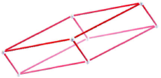
Figure 1: The oblate rhombohedron.

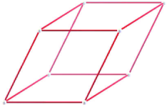
Figure 2: The prolate rhombohedron.

Consider now the vectors in $\big{(}\mbox{\bbb{R}}^{3}\big{)}^{*}$

$$\alpha_{1}=\tfrac{1}{\sqrt{2}}(\phi-1,1,0),\qquad \alpha_{2}=\tfrac{1}{\sqrt{2}}(0,\phi-1,1),\qquad \alpha_{3}=\tfrac{1}{\sqrt{2}}(1,0,\phi-1),$$

$$\alpha_{4}=\tfrac{1}{\sqrt{2}}(1-\phi,1,0),\qquad \alpha_{5}=\tfrac{1}{\sqrt{2}}(0,1-\phi,1),\qquad \alpha_{6}=\tfrac{1}{\sqrt{2}}(1,0,1-\phi).$$

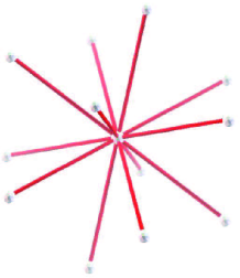
Figure 3: The vectors $\pm\alpha_{1},\ldots,\pm\alpha_{6}$.

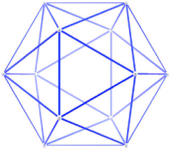
Figure 4: The icosahedron.

These six vectors and their opposites point to the twelve vertices of an icosahedron that is inscribed in the sphere of radius $\sqrt{\frac{3-\phi}{2}}$ (see Figs. 4 and 4); they generate a quasilattice $P$ that is known in physics as the simple icosahedral lattice [9].

Let $\delta=\sqrt{\frac{2}{3-\phi}}\sigma$ and consider the two following golden rhombohedra: the oblate rhombohedron $\Delta_{b}^{o}$, having nonparallel edges $\delta\alpha_{4}$, $\delta\alpha_{5}$, $\delta\alpha_{6}$, and the prolate rhombohedron $\Delta_{r}^{o}$, having nonparallel edges $\delta\alpha_{1}$, $\delta\alpha_{2}$, $\delta\alpha_{3}$.

Denote by $AB$ one edge of the tiling $\cal T$. From now on we will choose our coordinates so that $A=O$ and so that $B-A$ is parallel to $\alpha_{1}$ with the same orientation.

Proposition 3.1.

Let $\cal T$ be an Ammann tiling with edges of length $\sigma$. Each vertex of the tiling lies in the quasilattice $\delta P$. Moreover, for each oblate rhombohedron $\Delta_{b}$ in $\cal T$ $($respectively prolate rhombohedron $\Delta_{r}$ in $\cal T)$ there is a rigid motion $\rho$, given by the composition of a translation with a transformation of the icosahedral group, such that $\rho(\Delta_{b})$ is $\Delta_{b}^{o}$ $($respectively $\rho(\Delta_{r})$ is $\Delta_{r}^{o})$.

Proof 3.2.

Consider first the icosahedron with its twenty pairwise parallel facets. To each pair of parallel facets there correspond two oblate rhombohedra, one the translate of the other, and two prolate rhombohedra, also one the translate of the other. Pick one representative for each such couple. This gives a total of ten oblate rhombohedra and ten prolate rhombohedra. Each of the ten oblate rhombohedra can be mapped to $\Delta_{b}^{o}$ via a transformation of the icosahedral group, and in the same way each of the ten prolate rhombohedra can be mapped to $\Delta_{r}^{o}$.

Now, let $C$ be a vertex of the tiling that is different from $0$ and the above vertex $B$. We can join $B$ to $C$ with a broken line made of subsequent edges of the tiling. We denote the vertices of the broken line thus obtained by $T_{0}=A,T_{1}=B,\dots,T_{j},\dots,T_{m}=C$. Since the tiles are oblate and prolate rhombohedra, each vector $Y_{j}=T_{j}-T_{j-1}$ is one of the vectors $\pm\alpha_{k}$, $k=1,\ldots,6$. Therefore we have that $C-A=T_{m}-T_{0}=Y_{m}+\cdots+Y_{1}$. This implies that the vertex $C$ lies in $\delta P$, that each oblate rhombohedron having $C$ as vertex is the translate of one of the ten oblate rhombohedra described above and that each prolate rhombohedron having $C$ as vertex is the translate of one of the ten prolate rhombohedra described above. We can therefore conclude that, for each oblate rhombohedron $\Delta_{b}$ having $C$ as vertex, there exists a rigid motion $\rho$, given by the composition of a translation with a transformation of the icosahedral group, such that $\rho(\Delta_{b})=\Delta_{b}^{o}$. The same is true for the prolate rhombohedra.

We introduce now a quasilattice $F\subset\mbox{\bbb{R}}^{3}$ with respect to which all of the rhombohedra of the tiling are quasirational (cf. Remark 2.7). This is necessary in order to apply the generalized Delzant procedure simultaneously to all of the rhombohedra in the tiling. We take $F$ to be the quasilattice that is generated by the six vectors

$$U_{1}=\tfrac{1}{\sqrt{2}}(1,\phi-1,\phi),\qquad U_{2}=\tfrac{1}{\sqrt{2}}(\phi,1,\phi-1),\qquad U_{3}=\tfrac{1}{\sqrt{2}}(\phi-1,\phi,1),$$

$$U_{4}=\tfrac{1}{\sqrt{2}}(-1,\phi-1,\phi),\qquad U_{5}=\tfrac{1}{\sqrt{2}}(\phi,-1,\phi-1),\qquad U_{6}=\tfrac{1}{\sqrt{2}}(\phi-1,\phi,-1).$$

The quasilattice $F$ is known in physics as the face-centered lattice [9].

The vectors $U_{i}$ have norm equal to $\sqrt{2}$. It can be easily seen that there are exactly $30$ vectors in $F$ having the same norm. These thirty vectors point to the vertices of an icosidodecahedron inscribed in the sphere of radius $\sqrt{2}$ (see Figs. 6 and 6).

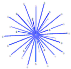
Figure 5: The star of norm $\sqrt{2}$ vectors of the quasilattice $F$.

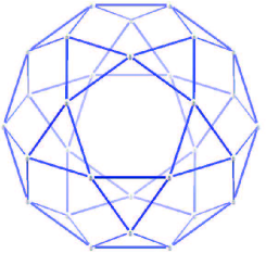
Figure 6: The icosidodecahedron.

Remark 3.3.

Proposition 3.1 implies that, for each facet of the Ammann tiling, there is a pair of vectors $\{\alpha_{i},\alpha_{j}\}$ such that the given facet is parallel to the plane $\Pi_{ij}$ generated by $\{\alpha_{i},\alpha_{j}\}$. We have $15$ such possible pairs $\{\alpha_{i},\alpha_{j}\}$, with $i,j=1,\ldots,6$, $i\neq j$. For each one of them, two of the $30$ vectors above are orthogonal to the corresponding plane $\Pi_{ij}$. This ensures that all of the rhombohedra of the tiling are quasirational with respect to $F$.

Another quasilattice that will be useful in the sequel is the quasilattice $I\subset\big{(}\mbox{\bbb{R}}^{3}\big{)}^{*}$ that is generated by the vectors $\{2\alpha_{1},2\alpha_{2},2\alpha_{3},2\phi\alpha_{4},2\phi\alpha_{5},2\phi\alpha_{6}\}$. The quasilattice $I$ is known in physics as the body centered lattice [9].

Remark 3.4.

The quasilattices $P$, $F$ and $I$ are invariant under icosahedral symmetries and are dense in their respective ambient spaces. One can show that, if we identify $\mbox{\bbb{R}}^{3}$ with its dual using the standard inner product, we have the following proper inclusions:

$$I\subset F\subset P\subset\tfrac{1}{2}I.$$ (3.2)

Using the notation of Conway–Sloane [4], the lattices $P$, $F$ and $\frac{1}{2}I$ can be obtained as the respective projections from the following lattices in $\mbox{\bbb{R}}^{6}$: $\mbox{\bbb{Z}}^{6}$,

$$D_{6}=\hbox{Span}\left\{\sum_{j=1}^{6}n_{j}e_{j}\;\Big{|}\;\sum_{j=1}^{6}n_{j}\;\hbox{is even}\right\},$$

and

$$D_{6}^{*}=\hbox{Span}\left\{\frac{1}{2}\sum_{j=1}^{6}n_{j}e_{j}\;\Big{|}\;n_{j}\equiv n_{k}\ (\hbox{mod}\,2)\right\},$$

the projection being given by

$${\mbox{\bbb{R}}^{6}} \longrightarrow\ \mbox{\bbb{R}}^{3}$$

$${e_{j}} \longmapsto\ \alpha_{j}.$$

Coherently with (3.2) we have the following proper inclusions:

$$2D_{6}^{*}\subset D_{6}\subset\mbox{\bbb{Z}}^{6}\subset D_{6}^{*}.$$

The lattice $\mbox{\bbb{Z}}^{6}$ is self dual, whilst $D_{6}$ and $D_{6}^{*}$ are the dual of one another. A notion of duality for the icosahedral quasilattices in dimension $3$ is derived from the above relations of duality in $\mbox{\bbb{R}}^{6}$. This is coherent with the symplectic setup. In fact, we will see that the quasilattice $F$ is the group quasilattice (see Remark 4.1) and that the quasilattice $\frac{1}{2}I$ plays the role of its dual, the weight quasilattice (see Section 5).

4 The tiling from a symplectic viewpoint

In this section we perform the Delzant construction to obtain symplectic quasifolds that can be associated to the oblate and prolate rhombohedra of an Ammann tiling having edge length $\sigma$.

Let us consider the quasilattice $F$ that we introduced in Section 3. As we have seen, all of the rhombohedra of our tiling are quasirational with respect to $F$.

We begin by considering the oblate rhombohedron $\Delta_{b}^{o}$ which has one of its vertices at the origin and is determined by the three non-parallel vectors $\delta\alpha_{4}$, $\delta\alpha_{5}$, $\delta\alpha_{6}$. This simple polytope has $6$ facets. For our construction we choose the $6$ vectors given by $X_{1}=U_{1}$, $X_{2}=U_{2}$, $X_{3}=U_{3}$, $X_{4}=-U_{1}$, $X_{5}=-U_{2}$ and $X_{6}=-U_{3}$. Then the corresponding coefficients are given by $\lambda_{1}=\lambda_{2}=\lambda_{3}=0$ and $\lambda_{4}=\lambda_{5}=\lambda_{6}=-\frac{\delta}{2\phi}$. Take now the surjective linear mapping defined by

$$\pi\colon\ \mbox{\bbb{R}}^{6} \rightarrow\ \mbox{\bbb{R}}^{3}$$

$$e_{i} \mapsto\ X_{i}.$$

Its kernel, $\mathfrak{n}$, is the $3$-dimensional subspace of $\mbox{\bbb{R}}^{6}$ that is spanned by $e_{1}+e_{4}$, $e_{2}+e_{5}$ and $e_{3}+e_{6}$. It is the Lie algebra of $N=\{\exp(X)\in T^{6}\,|\,X\in\mbox{\bbb{R}}^{6},\pi(X)\in F\}$. If $\Psi_{b}$ is the moment mapping of the induced $N$-action, then

$$\Psi_{b}\colon\ \mbox{\bbb{C}}^{6} \longrightarrow\ \big{(}\mbox{\bbb{R}}^{3}\big{)}^{*}$$

$$\underline{z} \longmapsto\ \left(|z_{1}|^{2}+|z_{4}|^{2}-\tfrac{\delta}{2\phi},|z_{2}|^{2}+|z_{5}|^{2}-\tfrac{\delta}{2\phi},|z_{3}|^{2}+|z_{6}|^{2}-\tfrac{\delta}{2\phi}\right).$$

Therefore $\Psi_{b}^{-1}(0)=S^{3}_{b}\times S^{3}_{b}\times S^{3}_{b}$, where $S^{3}_{b}$ is the sphere in $\mbox{\bbb{R}}^{4}$ centered at the origin with radius $b=\sqrt{\frac{\delta}{2\phi}}$. In order to compute the group $N$ we need the following linear relations between the generators of the quasilattice $F$:

$$\left(\begin{matrix}U_{4}\\ U_{5}\\ U_{6}\end{matrix}\right)=\left(\begin{matrix}1&-\phi&1\\ 1&1&-\phi\\ -\phi&1&1\end{matrix}\right)\left(\begin{matrix}U_{1}\\ U_{2}\\ U_{3}\end{matrix}\right).$$

Then a straightforward computation gives that

$$N=\left\{\exp(X)\in T^{6}\,|\,X=(r+\phi h,s+\phi k,t+\phi l,r,s,t),\,r,s,t\in\mbox{\bbb{R}},\,h,k,l\in\mbox{\bbb{Z}}\right\}.$$

We can think of

$$S^{1}\times S^{1}\times S^{1}=\big{\{}\exp(X)\in T^{6}\,|\,X=(r,s,t,r,s,t),\,r,s,t\in\mbox{\bbb{R}}\big{\}}$$ (4.1)

as being naturally embedded in $N$. The quotient group

$$\Gamma=\frac{N}{S^{1}\times S^{1}\times S^{1}}$$

is discrete. In conclusion, the symplectic quotient $M_{b}$ is given by

$$M_{b}=\frac{\Psi_{b}^{-1}(0)}{N}=\frac{S^{3}_{b}\times S^{3}_{b}\times S^{3}_{b}}{N}=\frac{S^{2}_{b}\times S^{2}_{b}\times S^{2}_{b}}{\Gamma},$$

where $S^{2}_{b}$ is the sphere in $\mbox{\bbb{R}}^{3}$ centered at the origin with radius $b$. The quasitorus $D^{3}=\mbox{\bbb{R}}^{3}/F$ acts on $M_{b}$ in a Hamiltonian fashion, with image of the corresponding moment mapping given exactly by the oblate rhombohedron $\Delta_{b}^{o}$.

Consider now the prolate rhombohedron $\Delta_{r}^{o}$ that has one vertex in the origin and is determined by the three nonparallel vectors $\delta\alpha_{1}$, $\delta\alpha_{2}$, $\delta\alpha_{3}$. We now choose the vectors given by $X_{1}=U_{4}$, $X_{2}=U_{5}$, $X_{3}=U_{6}$, $X_{4}=-U_{4}$, $X_{5}=-U_{5}$ and $X_{6}=-U_{6}$. Then the corresponding coefficients are given by $\lambda_{1}=\lambda_{2}=\lambda_{3}=0$ and $\lambda_{4}=\lambda_{5}=\lambda_{6}=-\frac{\delta}{2}$. It is immediate to check that we obtain the same Lie algebra $\mathfrak{n}$ as in the case of the oblate rhombohedron. In order to see what happens to the corresponding group we need here the inverse relations:

$$\left(\begin{matrix}U_{1}\\ U_{2}\\ U_{3}\end{matrix}\right)=\left(\begin{matrix}1&1&\frac{1}{\phi}\\ \frac{1}{\phi}&1&1\\ 1&\frac{1}{\phi}&1\end{matrix}\right)\left(\begin{matrix}U_{4}\\ U_{5}\\ U_{6}\end{matrix}\right).$$

To write the relations in this form we used the fundamental identity (3.1). This identity also implies that we obtain the same group $N$ as in the case of the oblate rhombohedron.

The moment mapping $\Psi_{r}$ is given by

$$\Psi_{r}\colon\ \mbox{\bbb{C}}^{6} \longrightarrow\ \big{(}\mbox{\bbb{R}}^{3}\big{)}^{*}$$

$$\underline{z} \longmapsto\ \left(|z_{1}|^{2}+|z_{4}|^{2}-\tfrac{\delta}{2},|z_{2}|^{2}+|z_{5}|^{2}-\tfrac{\delta}{2},|z_{3}|^{2}+|z_{6}|^{2}-\tfrac{\delta}{2}\right).$$

Therefore

$$M_{r}=\frac{\Psi_{r}^{-1}(0)}{N}=\frac{S^{3}_{r}\times S^{3}_{r}\times S^{3}_{r}}{N}=\frac{S^{2}_{r}\times S^{2}_{r}\times S^{2}_{r}}{\Gamma},$$

where $S^{2}_{r}\subset\mbox{\bbb{R}}^{3}$ and $S^{3}_{r}\subset\mbox{\bbb{R}}^{4}$ are the spheres centered at the origin with radius $r=\sqrt{\frac{\delta}{2}}$. The quasifold $M_{r}$ is acted on by the same quasitorus $D^{3}=\mbox{\bbb{R}}^{3}/F$ that we obtained for the oblate rhombohedron. This action is Hamiltonian and the image of the corresponding moment mapping is exactly the prolate rhombohedron $\Delta_{r}^{o}$.

Remark 4.1.

Let us remark that $M_{b}$ and $M_{r}$ are both global quotients and that this defines their quasifold structures. The quasilattice $F$ can be viewed as the group quasilattice of the quasitorus $D^{3}$ acting on both.

Remark now that, by Proposition 3.1, each of the oblate and prolate rhombohedra in the tiling can be obtained from $\Delta_{b}^{o}$ and $\Delta_{r}^{o}$ respectively by a transformation of the icosahedral group composed with a translation. We can then prove the following

Theorem 4.2.

Consider an Ammann tiling having edge length $\sigma$. Then the compact connected symplectic quasifold corresponding to each oblate rhombohedron in the tiling is given by $M_{b}$, while the compact connected symplectic quasifold corresponding to each prolate rhombohedron is given by $M_{r}$.

Proof 4.3.

Observe that, for each oblate rhombohedron, there exists a transformation $T$ in the icosahedral group that leaves the quasilattice $F$ invariant, that sends the orthogonal vectors relative to the chosen oblate rhombohedron to the orthogonal vectors relative to $\Delta_{b}^{o}$, and such that the dual transformation $T^{*}$ sends $\Delta_{b}^{o}$ to a translate of the chosen oblate rhombohedron. The same reasoning applies to the prolate rhombohedra of the tiling. This implies that the reduced space corresponding to each oblate rhombohedron of the tiling, with the choice of orthogonal vectors and quasilattice specified above, is exactly $M_{b}$. This yields a unique symplectic quasifold, $M_{b}$, for all the oblate rhombohedra in the tiling. In the same way we prove that we obtain a unique symplectic quasifold, $M_{r}$, for all the prolate rhombohedra in the tiling.

The quasifolds $M_{b}$ and $M_{r}$ can also be constructed as complex quotients and are Kähler [1].

5 Local geometry of the quasifolds $\boldsymbol{M_{b}}$ and $\boldsymbol{M_{r}}$

In this section we study the equivariant geometry of the quasifolds $M_{b}$ and $M_{r}$ in a neighborhood of the $D^{3}$-fixed points.

Let us begin by describing an atlas for the quasifold $M_{b}$. The charts of this atlas are indexed by the vertices of the polytope: in our case we find an atlas given by eight charts, each of which corresponds to a vertex of the oblate rhombohedron. Consider for example the origin: it is given by the intersection of the facets whose orthogonal vectors are $X_{1}$, $X_{2}$ and $X_{3}$. Let $B_{b}$ be the ball in ℂ of radius $b$, namely

$$B_{b}=\{z\in\mbox{\bbb{C}}\,|\,|z|<b\}.$$

Consider the following mapping, which gives a slice of $\Psi_{b}^{-1}(0)$ transversal to the $N$-orbits

$$B_{b}\times B_{b}\times B_{b} \stackrel{{\scriptstyle t_{1}}}{{\longrightarrow}}\ \big{\{}\underline{z}\in\Psi^{-1}_{b}(0)\,|\,z_{4}\neq 0,\,z_{5}\neq 0,\,z_{6}\neq 0\big{\}}$$

$$(z_{1},z_{2},z_{3}) \longmapsto\ \Big{(}z_{1},z_{2},z_{3},\sqrt{b^{2}-|z_{1}|^{2}},\sqrt{b^{2}-|z_{2}|^{2}},\sqrt{b^{2}-|z_{3}|^{2}}\Big{)}.$$

This induces the homeomorphism

$$(B_{b}\times B_{b}\times B_{b})/\Gamma_{1} \stackrel{{\scriptstyle\tau_{1}}}{{\longrightarrow}}\ U_{1}$$

$$[\underline{z}] \longmapsto\ [t_{1}(\underline{z})],$$

where the open subset $U_{1}$ of $M_{b}$ is the quotient

$$\big{\{}\underline{z}\in\Psi_{b}^{-1}(0)\,|\,z_{4}\neq 0,\,z_{5}\neq 0,\,z_{6}\neq 0\big{\}}/N$$

and the discrete group $\Gamma_{1}$ is given by $\Gamma_{1}\simeq N\cap(S^{1}\times S^{1}\times S^{1}\times\{1\}\times\{1\}\times\{1\}),$ hence

$$\Gamma_{1}=\exp\left\{\left(\phi h,\phi k,\phi l\right)\,|\,h,k,l\in\mbox{\bbb{Z}}\right\}.$$ (5.1)

The triple $(U_{1},\tau_{1},(B_{b}\times B_{b}\times B_{b})/\Gamma_{1})$ is a chart of $M_{b}$. Analogously, we can construct seven other charts, corresponding to the remaining vertices of the oblate rhombohedron, each of which is characterized by a different combination of the variables. One can show that these eight charts are compatible and give an atlas of $M_{b}$.

One can check that the moment map, locally, on the first chart is given by

$$\Phi([z_{1}:z_{2}:z_{3}])=\frac{\phi\alpha_{5}}{\langle\phi\alpha_{5},U_{1}\rangle}|z_{1}|^{2}+\frac{\phi\alpha_{6}}{\langle\phi\alpha_{6},U_{2}\rangle}|z_{2}|^{2}+\frac{\phi\alpha_{4}}{\langle\phi\alpha_{4},U_{3}\rangle}|z_{3}|^{2}$$

$$\phantom{\Phi([z_{1}:z_{2}:z_{3}])}=\phi\alpha_{5}|z_{1}|^{2}+\phi\alpha_{6}|z_{2}|^{2}+\phi\alpha_{4}|z_{3}|^{2},$$

while the isotropy action of $D^{3}$ on $\mbox{\bbb{C}}^{3}/\Gamma_{1}$ is given by

$$\big{(}D^{3},\mbox{\bbb{C}}^{3}/\Gamma_{1}\big{)} \longrightarrow\ \mbox{\bbb{C}}^{3}/\Gamma_{1}$$

$$([X],(z_{1},z_{2},z_{3})) \longmapsto\ \big{(}e^{2\pi i\phi\alpha_{5}(X)}z_{1},e^{2\pi i\phi\alpha_{6}(X)}z_{2},e^{2\pi i\phi\alpha_{4}(X)}z_{3}\big{)}.$$ (5.2)

To obtain the local expression of the moment mapping on the other seven charts it suffices to replace $\phi\alpha_{5}$, $\phi\alpha_{6}$, $\phi\alpha_{4}$ in (5.2) with all the possible combinations of $\pm\phi\alpha_{5}$, $\pm\phi\alpha_{6}$, $\pm\phi\alpha_{4}$ respectively. Notice that the vectors $U_{1}$, $U_{2}$, $U_{3}$ are three of the six generators of $F$, while $\phi\alpha_{4}$, $\phi\alpha_{5}$, $\phi\alpha_{6}$ are three of the six generators of $\frac{1}{2}I$.

An atlas for the the quasifold $M_{r}$ can be constructed in the same way. It can be shown that the moment mapping for the prolate rhomobohedron, is given, locally on the chart corresponding to the origin, by

$$\Phi([z_{1}:z_{2}:z_{3}])=\frac{\alpha_{2}}{\langle\alpha_{2},U_{4}\rangle}|z_{1}|^{2}\!+\frac{\alpha_{3}}{\langle\alpha_{3},U_{5}\rangle}|z_{2}|^{2}\!+\frac{\alpha_{1}}{\langle\alpha_{1},U_{6}\rangle}|z_{3}|^{2}=\alpha_{2}|z_{1}|^{2}\!+\alpha_{3}|z_{2}|^{2}\!+\alpha_{1}|z_{3}|^{2},$$

while the isotropy action of $D^{3}$ on $\mbox{\bbb{C}}^{3}/\Gamma_{1}$ is given by

$$\big{(}D^{3},\mbox{\bbb{C}}^{3}/\Gamma_{1}\big{)} \longrightarrow\ \mbox{\bbb{C}}^{3}/\Gamma_{1}$$

$$([X],(z_{1},z_{2},z_{3})) \longmapsto\ \big{(}e^{2\pi i\alpha_{2}(X)}z_{1},e^{2\pi i\alpha_{3}(X)}z_{2},e^{2\pi i\alpha_{1}(X)}z_{3}\big{)}.$$

Again, notice that the vectors $U_{4}$, $U_{5}$, $U_{6}$ are the three remaining generators of $F$, while $\alpha_{1}$, $\alpha_{2}$, $\alpha_{3}$ are the three remaining generators of $\frac{1}{2}I$. In conclusion, the weights of the isotropy action of the quasitorus $D^{3}$ on a neighboorhood of the $D^{3}$-fixed points for both $M_{b}$ and $M_{r}$ generate the quasilattice $\frac{1}{2}I$. Therefore $\frac{1}{2}I$ can be thought of, in this setting, as the weight quasilattice of $D^{3}$. This is consistent with the fact that $\frac{1}{2}I$ is dual to the group quasilattice $F$ (cf. Remark 3.4).

Remark 5.1.

Remark that, since $\alpha_{i}(X)$, $\phi\alpha_{i}(X)$ lie in $\mbox{\bbb{Z}}+\phi\mbox{\bbb{Z}}$ whenever $X\in F$, and since the local group in each chart of $M_{b}$ and $M_{r}$ is equal to $\Gamma_{1}$, the above actions are well defined.

Remark 5.2.

If we choose as group lattice $tF$ instead, $t\in\mbox{\bbb{R}}$, then the corresponding weight lattice would have to be $\frac{1}{2t}I$. But this would not be consistent with the inclusion and projection schemes in Remark 3.4. This is the main reason underlying our choice of the norm of the vectors $\alpha_{j}$, $j=1,\ldots,6$.

6 Diffeotype and symplectotype of the tiles

The purpose of this section is to prove the following

Theorem 6.1.

The quasifolds $M_{b}$ and $M_{r}$ are diffeomorphic but not symplectomorphic.

Before proceeding with the proof of this theorem we need a few more facts on the local geometry of the quasifold $M_{b}$. Let us denote by $p_{b}$ the projection

$$S^{2}_{b}\times S^{2}_{b}\times S^{2}_{b}\rightarrow M_{b}.$$

Denote by $V_{n}$ the open subset of $S^{2}_{b}$ given by $S^{2}_{b}$ minus the south pole and by $V_{s}$ the open subset of $S^{2}_{b}$ given by $S^{2}_{b}$ minus the north pole. Then, on $\Psi_{b}^{-1}(0)$, consider the action of $S^{1}\times S^{1}\times S^{1}$ given by (4.1). We obtain

$$V_{n}\times V_{n}\times V_{n}=\big{\{}\underline{z}\in\Psi_{b}^{-1}(0)\,|\,z_{4}\neq 0,\,z_{5}\neq 0,\,z_{6}\neq 0\big{\}}/\big{(}S^{1}\times S^{1}\times S^{1}\big{)}$$

and

$$U_{1}=(V_{n}\times V_{n}\times V_{n})/\Gamma.$$

We have the following commutative diagram:

$$\begin{gathered}\lx@xy@svg{\hbox{\raise 0.0pt\hbox{\kern 41.87126pt\hbox{\ignorespaces\ignorespaces\ignorespaces\hbox{\vtop{\kern 0.0pt\offinterlineskip\halign{\entry@#!@&&\entry@@#!@\cr&\\&\\&\crcr}}}\ignorespaces{\hbox{\kern-28.73518pt\raise 0.0pt\hbox{\hbox{\kern 0.0pt\raise 0.0pt\hbox{\hbox{\kern 3.0pt\raise 0.0pt\hbox{$\textstyle{B_{b}\times B_{b}\times B_{b}\ignorespaces\ignorespaces\ignorespaces\ignorespaces\ignorespaces\ignorespaces\ignorespaces\ignorespaces}$}}}}}}}\ignorespaces\ignorespaces\ignorespaces\ignorespaces{}{\hbox{\lx@xy@droprule}}\ignorespaces\ignorespaces\ignorespaces{\hbox{\kern 39.60738pt\raise 5.79723pt\hbox{{}\hbox{\kern 0.0pt\raise 0.0pt\hbox{\hbox{\kern 3.0pt\hbox{\hbox{\kern 0.0pt\raise-1.50835pt\hbox{$\scriptstyle{t_{1}}$}}}\kern 3.0pt}}}}}}\ignorespaces{\hbox{\kern 65.87126pt\raise 0.0pt\hbox{\hbox{\kern 0.0pt\raise 0.0pt\hbox{\lx@xy@tip{1}\lx@xy@tip{-1}}}}}}{\hbox{\lx@xy@droprule}}{\hbox{\lx@xy@droprule}}\ignorespaces\ignorespaces\ignorespaces\ignorespaces{}{\hbox{\lx@xy@droprule}}\ignorespaces{\hbox{\kern 0.0pt\raise-30.12444pt\hbox{\hbox{\kern 0.0pt\raise 0.0pt\hbox{\lx@xy@tip{1}\lx@xy@tip{-1}}}}}}{\hbox{\lx@xy@droprule}}{\hbox{\lx@xy@droprule}}{\hbox{\kern 65.87126pt\raise 0.0pt\hbox{\hbox{\kern 0.0pt\raise 0.0pt\hbox{\hbox{\kern 3.0pt\raise 0.0pt\hbox{$\textstyle{\big{\{}\underline{z}\in\Psi_{b}^{-1}(0)\,|\,z_{4}\neq 0,\,z_{5}\neq 0,\,z_{6}\neq 0\big{\}}\ignorespaces\ignorespaces\ignorespaces\ignorespaces}$}}}}}}}\ignorespaces\ignorespaces\ignorespaces\ignorespaces{}{\hbox{\lx@xy@droprule}}\ignorespaces{\hbox{\kern 138.71373pt\raise-30.12444pt\hbox{\hbox{\kern 0.0pt\raise 0.0pt\hbox{\lx@xy@tip{1}\lx@xy@tip{-1}}}}}}{\hbox{\lx@xy@droprule}}{\hbox{\lx@xy@droprule}}{\hbox{\kern-28.73518pt\raise-39.95775pt\hbox{\hbox{\kern 0.0pt\raise 0.0pt\hbox{\hbox{\kern 3.0pt\raise 0.0pt\hbox{$\textstyle{B_{b}\times B_{b}\times B_{b}\ignorespaces\ignorespaces\ignorespaces\ignorespaces\ignorespaces\ignorespaces\ignorespaces\ignorespaces}$}}}}}}}\ignorespaces\ignorespaces\ignorespaces\ignorespaces{}{\hbox{\lx@xy@droprule}}\ignorespaces\ignorespaces\ignorespaces{\hbox{\kern 62.57907pt\raise-32.7022pt\hbox{{}\hbox{\kern 0.0pt\raise 0.0pt\hbox{\hbox{\kern 3.0pt\hbox{\hbox{\kern 0.0pt\raise-2.96667pt\hbox{$\scriptstyle{\tilde{\tau}_{1}}$}}}\kern 3.0pt}}}}}}\ignorespaces{\hbox{\kern 108.58846pt\raise-39.95775pt\hbox{\hbox{\kern 0.0pt\raise 0.0pt\hbox{\lx@xy@tip{1}\lx@xy@tip{-1}}}}}}{\hbox{\lx@xy@droprule}}{\hbox{\lx@xy@droprule}}\ignorespaces\ignorespaces\ignorespaces\ignorespaces{}{\hbox{\lx@xy@droprule}}\ignorespaces\ignorespaces\ignorespaces{\hbox{\kern-11.52188pt\raise-59.65218pt\hbox{{}\hbox{\kern 0.0pt\raise 0.0pt\hbox{\hbox{\kern 3.0pt\hbox{\hbox{\kern 0.0pt\raise-0.8264pt\hbox{$\scriptstyle{p_{1}}$}}}\kern 3.0pt}}}}}}\ignorespaces{\hbox{\kern 0.0pt\raise-68.84662pt\hbox{\hbox{\kern 0.0pt\raise 0.0pt\hbox{\lx@xy@tip{1}\lx@xy@tip{-1}}}}}}{\hbox{\lx@xy@droprule}}{\hbox{\lx@xy@droprule}}{\hbox{\kern 108.58846pt\raise-39.95775pt\hbox{\hbox{\kern 0.0pt\raise 0.0pt\hbox{\hbox{\kern 3.0pt\raise 0.0pt\hbox{$\textstyle{V_{n}\times V_{n}\times V_{n}\ignorespaces\ignorespaces\ignorespaces\ignorespaces}$}}}}}}}\ignorespaces\ignorespaces\ignorespaces\ignorespaces{}{\hbox{\lx@xy@droprule}}\ignorespaces\ignorespaces\ignorespaces{\hbox{\kern 138.71373pt\raise-59.65218pt\hbox{{}\hbox{\kern 0.0pt\raise 0.0pt\hbox{\hbox{\kern 3.0pt\hbox{\hbox{\kern 0.0pt\raise-0.8125pt\hbox{$\scriptstyle{p_{b}}$}}}\kern 3.0pt}}}}}}\ignorespaces{\hbox{\kern 138.71373pt\raise-69.5133pt\hbox{\hbox{\kern 0.0pt\raise 0.0pt\hbox{\lx@xy@tip{1}\lx@xy@tip{-1}}}}}}{\hbox{\lx@xy@droprule}}{\hbox{\lx@xy@droprule}}{\hbox{\kern-41.87126pt\raise-79.34662pt\hbox{\hbox{\kern 0.0pt\raise 0.0pt\hbox{\hbox{\kern 3.0pt\raise 0.0pt\hbox{$\textstyle{(B_{b}\times B_{b}\times B_{b})/\Gamma_{1}\ignorespaces\ignorespaces\ignorespaces\ignorespaces}$}}}}}}}\ignorespaces\ignorespaces\ignorespaces\ignorespaces{}{\hbox{\lx@xy@droprule}}\ignorespaces\ignorespaces\ignorespaces{\hbox{\kern 63.82683pt\raise-74.19524pt\hbox{{}\hbox{\kern 0.0pt\raise 0.0pt\hbox{\hbox{\kern 3.0pt\hbox{\hbox{\kern 0.0pt\raise-0.8625pt\hbox{$\scriptstyle{\tau_{1}}$}}}\kern 3.0pt}}}}}}\ignorespaces{\hbox{\kern 128.96582pt\raise-79.34662pt\hbox{\hbox{\kern 0.0pt\raise 0.0pt\hbox{\lx@xy@tip{1}\lx@xy@tip{-1}}}}}}{\hbox{\lx@xy@droprule}}{\hbox{\lx@xy@droprule}}{\hbox{\kern 128.96582pt\raise-79.34662pt\hbox{\hbox{\kern 0.0pt\raise 0.0pt\hbox{\hbox{\kern 3.0pt\raise 0.0pt\hbox{$\textstyle{U_{1}.}$}}}}}}}\ignorespaces}}}}\ignorespaces\end{gathered} \textstyle{B_{b}\times B_{b}\times B_{b}\ignorespaces\ignorespaces\ignorespaces\ignorespaces\ignorespaces\ignorespaces\ignorespaces\ignorespaces} \scriptstyle{t_{1}} \textstyle{\big{\{}\underline{z}\in\Psi_{b}^{-1}(0)\,|\,z_{4}\neq 0,\,z_{5}\neq 0,\,z_{6}\neq 0\big{\}}\ignorespaces\ignorespaces\ignorespaces\ignorespaces} \textstyle{B_{b}\times B_{b}\times B_{b}\ignorespaces\ignorespaces\ignorespaces\ignorespaces\ignorespaces\ignorespaces\ignorespaces\ignorespaces} \scriptstyle{\tilde{\tau}_{1}} \scriptstyle{p_{1}} \textstyle{V_{n}\times V_{n}\times V_{n}\ignorespaces\ignorespaces\ignorespaces\ignorespaces} \scriptstyle{p_{b}} \textstyle{(B_{b}\times B_{b}\times B_{b})/\Gamma_{1}\ignorespaces\ignorespaces\ignorespaces\ignorespaces} \scriptstyle{\tau_{1}} \textstyle{U_{1}.} \textstyle{B_{b}\times B_{b}\times B_{b}\ignorespaces\ignorespaces\ignorespaces\ignorespaces\ignorespaces\ignorespaces\ignorespaces\ignorespaces} \scriptstyle{t_{1}} \textstyle{\big{\{}\underline{z}\in\Psi_{b}^{-1}(0)\,|\,z_{4}\neq 0,\,z_{5}\neq 0,\,z_{6}\neq 0\big{\}}\ignorespaces\ignorespaces\ignorespaces\ignorespaces} \textstyle{B_{b}\times B_{b}\times B_{b}\ignorespaces\ignorespaces\ignorespaces\ignorespaces\ignorespaces\ignorespaces\ignorespaces\ignorespaces} \scriptstyle{\tilde{\tau}_{1}} \scriptstyle{p_{1}} \textstyle{V_{n}\times V_{n}\times V_{n}\ignorespaces\ignorespaces\ignorespaces\ignorespaces} \scriptstyle{p_{b}} \textstyle{(B_{b}\times B_{b}\times B_{b})/\Gamma_{1}\ignorespaces\ignorespaces\ignorespaces\ignorespaces} \scriptstyle{\tau_{1}} \textstyle{U_{1}.}$$ (6.8)

The mapping $\tilde{\tau}_{1}$ is induced by the diagram and can be written as $\tau_{n}\times\tau_{n}\times\tau_{n}$, with $\tau_{n}\colon B_{b}\rightarrow V_{n}$. Observe that the mapping

ℂ $$\longrightarrow\ V_{n}$$

$$w \longmapsto\ \big{[}\tau_{n}\big{(}bw/\sqrt{1+|w|^{2}}\big{)}\big{]}$$

is just the stereographic projection from the north pole. We denote by $\tau_{s}$ the analogous mapping $\tau_{s}\colon B_{b}\longrightarrow V_{s}$. The two charts $(B_{b},\tau_{n},V_{n})$ and $(B_{b},\tau_{s},V_{s})$ give a symplectic atlas of $S^{2}_{b}$, whose standard symplectic structure is induced by the standard symplectic structure on $B_{b}$. Analogously, at a local level, the symplectic structure of the quotient $M_{b}$ is induced by the standard symplectic structure on $B_{b}\times B_{b}\times B_{b}$.

We have already seen that the quasifold $M_{b}$ is a global quotient of a product of three $2$-spheres by the discrete group $\Gamma$. We remark that the atlas above is the quotient by $\Gamma$ of the atlas of the product of three spheres, given by the eight triples $V_{n}\times V_{n}\times V_{n}$, $V_{n}\times V_{n}\times V_{s}$, $V_{n}\times V_{s}\times V_{n}$, $V_{s}\times V_{n}\times V_{n}$, $V_{n}\times V_{s}\times V_{s}$, $V_{s}\times V_{n}\times V_{s}$, $V_{s}\times V_{s}\times V_{n}$, $V_{s}\times V_{s}\times V_{s}$.

We are now ready to prove Theorem 6.1:

Proof 6.2.

Let us begin by showing that $M_{b}$ and $M_{r}$ are diffeomorphic. Let us denote by $p_{r}$ the projection

$$S^{2}_{r}\times S^{2}_{r}\times S^{2}_{r}\rightarrow M_{r}.$$

The natural $\Gamma$-equivariant diffeomorphism $f^{\dagger}\colon S^{2}_{b}\times S^{2}_{b}\times S^{2}_{b}\rightarrow S^{2}_{r}\times S^{2}_{r}\times S^{2}_{r}$ induces a homeomorphism $f\colon M_{b}\rightarrow M_{r}$; in general, a homeomorphism between two global quotients that is induced by an equivariant diffeomorphism of the manifolds turns out to be a quasifold diffeomorphism [3, Definition A.2].

Let us now show that $M_{b}$ and $M_{r}$ are not symplectomorphic. Denote by $\omega_{b}$ and $\omega_{r}$ the symplectic forms of $M_{b}$ and $M_{r}$ respectively. Suppose that there is a symplectomorphism $h\colon M_{b}\longrightarrow M_{r}$, namely a diffeomorphism $h$ such that $h^{*}(\omega_{r})=\omega_{b}$. We prove that this implies that the homeomorphism $h\colon M_{b}\rightarrow M_{r}$ lifts to a symplectomorphism $\tilde{h}\colon S^{2}_{b}\times S^{2}_{b}\times S^{2}_{b}\rightarrow S^{2}_{r}\times S^{2}_{r}\times S^{2}_{r}$, leading thus to a contradiction: such symplectomorphism cannot exists, since the two manifolds have different symplectic volumes. To start with recall from [3, Remark 2.9] that, to each point $m\in M_{b}$, one can associate the groups $\Gamma_{m}$ and $\Gamma_{h(m)}$. The definition of diffeomorphism implies that these two groups are isomorphic. Let $n_{b}\in S^{2}_{b}$ be the north pole and take $m_{0}=p_{b}(n_{b}\times n_{b}\times n_{b})$. Then, since $\Gamma_{m}\simeq\Gamma_{h(m)}$, without loss of generality the point $h(m_{0})$ can be taken to be $p_{r}(n_{r}\times n_{r}\times n_{r})$, where $n_{r}\in S^{2}_{r}$ is the north pole. Consider the chart $U_{1}$ that we constructed above. Then, by definition of quasifold diffeomorphism [3, Definition A.23] and [3, Remark A.24], there exists an open subset $U\subset U_{1}$ such that $m_{0}\in U$ and $h\circ\tau_{1}^{-1}\colon\tau_{1}^{-1}(U)\rightarrow h(U)$ is a diffeomorphism of the universal covering models induced by $\tau_{1}^{-1}(U)\subset B_{b}\times B_{b}\times B_{b}/\Gamma_{1}$ and $h(U)\subset M_{r}$ respectively. Moreover, by [3, Proposition A.9], any open subset $W\subset U$ enjoys the same property. We can choose $W_{0}\subset U_{1}$ such that $\tilde{W}_{0}=(\tau_{1}\circ p_{1})^{-1}(W_{0}))$ is a product of three balls. In particular, $\tilde{W}_{0}$ is simply connected. Denote now by $\tilde{W}_{r,0}=(p_{r})^{-1}(h(W)))$; this is an open subset of $S^{2}_{r}\times S^{2}_{r}\times S^{2}_{r}$, which is also connected, due to the action of $\Gamma$ on $S^{2}_{r}\times S^{2}_{r}\times S^{2}_{r}$. Denote by $W^{\sharp}_{r,0}$ its universal covering. Now consider a point $\underline{z}^{1}\in B_{b}\times B_{b}\times B_{b}$ such that $z_{1}^{1}\neq 0$, $z_{2}^{1}\neq 0$ and $z_{3}^{1}\neq 0$ and let $m=(\tau_{1}\circ p_{1})(\underline{z}^{1})$. For the sequel it is crucial to remark that, because of the action of $\Gamma_{1}$ given in (5.1), any $\Gamma_{1}$-invariant open subset of $B_{b}\times B_{b}\times B_{b}$ that contains the point $\underline{z}^{1}$, contains also the product of circles $\{(z_{1},z_{2},z_{3})\in B_{b}\times B_{b}\times B_{b}\,|\,|z_{1}|=|z^{1}_{1}|,\,|z_{2}|=|z^{2}_{1}|,\,|z_{3}|=|z^{3}_{1}|\}$. Hence, for each point $(\tau_{1}\circ p_{1})(t\underline{z}^{1})$ with $t\in[0,1]$, we can find an open subset $W_{t}\subset U_{1}$, containing that point, such that the homeomorphism $\tau_{1}^{-1}\circ h$, restricted to $\tau_{1}^{-1}(W_{t})$, is a diffeomorphism, and $(\tau_{1}\circ p_{1})^{-1}(W_{t})$ is the product of three open annuli. We can cover the curve by a finite number of these $W_{t}$’s: $W_{0},W_{1},\ldots,W_{s}$, with $W_{j}\cap W_{j+1}\neq\varnothing$. Notice that $(\tau_{1}\circ p_{1})^{-1}(W_{j}\cap W_{j+1})$, $j=0,\ldots,s-1$, is itself a product of three open annuli. The subsets $\tilde{W}_{j}=(\tau_{1}\circ p_{1})^{-1}(W_{j})$ and $\tilde{W}_{r,j}=(p_{r})^{-1}(h(W_{j}))$ are open and connected.

We divide the remaining part of the proof in subsequent steps:

Step 1: consider first $W_{0}$. Since the isotropy of $\Gamma_{1}$ at $0$ is the whole $\Gamma_{1}$, we can apply [3, Lemma 6.2]. We find that $\tilde{W}_{r,0}$ is itself simply connected and that the homeomorphism $h\circ\tau_{1}$ lifts to a diffeomorphism $\tilde{h_{0}}\,\colon\,\tilde{W}_{0}\rightarrow\tilde{W}_{r,0}$.

Step 2: consider the homeomorphism $h_{1}=h\circ\tau_{1}$ defined on $\tau_{1}^{-1}(W_{1})$. By construction $h_{1}$ is a diffeomorphism of the universal covering models of the induced models. We find the following diagram:

Consider the restriction of $h_{1}$ to $\tau_{1}^{-1}(W_{0}\cap W_{1})$. This restriction admits a lift, given by the restriction of $h^{\sharp}_{1}$ to $(\pi_{1}\circ p_{1})^{-1}(\tau_{1}^{-1}(W_{0}\cap W_{1}))$. Furthermore, by Step 1, the restriction of $h_{1}$ admits another lift, defined on $p_{1}^{-1}(\tau_{1}^{-1}(W_{0}\cap W_{1}))$, which is the restriction of $\tilde{h}_{0}$. Therefore, by [3, Lemma 6.3], the restriction of $\rho_{1}\circ h_{1}^{\sharp}$ to $(\pi_{1}\circ p_{1})^{-1}(\tau_{1}^{-1}(W_{0}\cap W_{1}))$ descends to a diffeomorphism defined on $p_{1}^{-1}(\tau_{1}^{-1}(W_{0}\cap W_{1}))$.

Step 3: we consider $W_{0}\cap W_{1}\subset W_{1}$ and we apply [3, Lemma 6.5] to the homeomorphism $h\circ\tau_{1}$ defined on $\tau_{1}^{-1}(W_{1})$. We deduce that $h\circ\tau_{1}$ is a diffeomorphism of the model $(\tau_{1}\circ p_{1})^{-1}(W_{1})/\Gamma_{1}$ with the model induced by $h(W_{1})\subset M_{r}$.

Step 4: we apply Step 3 to the other successive intersections. We find that $h\circ\tau_{1}$ is a diffeomorphism of the model $(\tau_{1}\circ p_{1})^{-1}(\mathop{\cup}\limits_{i=1}^{k}W_{i})/\Gamma_{1}$ with the model induced by $h(\mathop{\cup}\limits_{i=1}^{k}W_{i})\subset M_{r}$. Remark now that a slight modification of the above argument applies to any choice of point $\underline{z}^{1}\in B_{b}\times B_{b}\times B_{b}$, $\underline{z}_{1}\neq 0$.

Let $\epsilon>0$ be arbitrarily small. Consider the product of closed balls $\overline{B}_{b-\epsilon}\times\overline{B}_{b-\epsilon}\times\overline{B}_{b-\epsilon}$. This, by Step 4, can be covered by a finite number of connected open subsets of the kind $(\tau_{1}\circ p_{1})^{-1}(\mathop{\cup}\limits_{i=1}^{k}W_{i})/\Gamma_{1}$, whose intersection is a product of three balls centered at the origin. Now [3, Lemma A.3], which guarantees the uniqueness of the lift up to the action of $\Gamma$, implies that the homeomorphism $h$ admits a lift to $\tilde{\tau}_{1}(\overline{B}_{b-\epsilon}\times\overline{B}_{b-\epsilon}\times\overline{B}_{b-\epsilon})$. This in turn implies that $h\colon U_{1}\rightarrow h(U_{1})$ admits a lift

$$\tilde{h}_{1}\colon\ V_{n}\times V_{n}\times V_{n}\rightarrow p_{r}^{-1}(h(U_{1})).$$

We apply the same argument to the other eight charts. These charts intersect on the dense connected open subset where the action of the quasitorus $D^{3}$ is free. By the uniqueness of the lift [3, Lemma A.3], we obtain a global lift $\tilde{h}\,\colon\,S^{2}_{b}\times S^{2}_{b}\times S^{2}_{b}\rightarrow S^{2}_{r}\times S^{2}_{r}\times S^{2}_{r}$. Moreover, since diagram (6.8) preserves the symplectic structures, we have that $\tilde{h}$ is a symplectomorphism between $S^{2}_{b}\times S^{2}_{b}\times S^{2}_{b}$ to $S^{2}_{r}\times S^{2}_{r}\times S^{2}_{r}$, which is impossible.

In conclusion, similarly to what happens in dimension two for Penrose rhombus tilings [2], there is a unique quasifold structure that is naturally associated to any Ammann tiling with fixed edge length, and two distinct symplectic structures that distinguish the oblate and the prolate rhombohedra.

Acknowledgements

We would like to thank Ron Lifshitz for his help on the theory of quasicrystals.

References

- [1] Battaglia F., Prato E., Generalized toric varieties for simple nonrational convex polytopes, Int. Math. Res. Not. (2001), 1315–1337, math.CV/0004066.
- [2] Battaglia F., Prato E., The symplectic geometry of Penrose rhombus tilings, J. Symplectic Geom. 6 (2008), 139–158, arXiv:0711.1642.
- [3] Battaglia F., Prato E., The symplectic Penrose kite, Comm. Math. Phys. 299 (2010), 577–601, arXiv:0712.1978.
- [4] Conway J.H., Sloane N.J.A., Sphere packings, lattices and groups, Grundlehren der Mathematischen Wissenschaften, Vol. 290, 3rd ed., Springer-Verlag, New York, 1999.
- [5] Delzant T., Hamiltoniens périodiques et images convexes de l’application moment, Bull. Soc. Math. France 116 (1988), 315–339.
- [6] Levine D., Steinhardt P.J., Quasicrystals: a new class of ordered structures, Phys. Rev. Lett. 53 (1984), 2477–2480.
- [7] Mackay A.L., De nive quinquangula: on the pentagonal snowflake, Sov. Phys. Cryst. (1981), 517–522.
- [8] Prato E., Simple non-rational convex polytopes via symplectic geometry, Topology 40 (2001), 961–975, math.SG/9904179.
- [9] Rokhsar D.S., Mermin N.D., Wright D.C., Rudimentary quasicrystallography: the icosahedral and decagonal reciprocal lattices, Phys. Rev. B 35 (1987), 5487–5495.
- [10] Senechal M., The mysterious Mr. Ammann, Math. Intelligencer 26 (2004), 10–21.
- [11] Shechtman D., Blech I., Gratias D., Cahn J.W., Metallic phase with long-range orientational order and no translational symmetry, Phys. Rev. Lett. 53 (1984), 1951–1953.
- [12] Steurer W., Deloudi S., Crystallography of quasicrystals: concepts, methods and structures, Springer Series in Materials Science, Vol. 126, Springer-Verlag, Berlin, 2009.