Fast solitons on star graphs

Abstract

We define the Schrödinger equation with focusing, cubic nonlinearity on one-vertex graphs. We prove global well-posedness in the energy domain and conservation laws for some self-adjoint boundary conditions at the vertex, i.e. Kirchhoff boundary condition and the so called $\delta$ and $\delta^{\prime}$ boundary conditions. Moreover, in the same setting we study the collision of a fast solitary wave with the vertex and we show that it splits in reflected and transmitted components. The outgoing waves preserve a soliton character over a time which depends on the logarithm of the velocity of the ingoing solitary wave. Over the same timescale the reflection and transmission coefficients of the outgoing waves coincide with the corresponding coefficients of the linear problem. In the analysis of the problem we follow ideas borrowed from the seminal paper [17] about scattering of fast solitons by a delta interaction on the line, by Holmer, Marzuola and Zworski; the present paper represents an extension of their work to the case of graphs and, as a byproduct, it shows how to extend the analysis of soliton scattering by other point interactions on the line, interpreted as a degenerate graph.

Keywords: quantum graphs, non-linear Schrödinger equation, solitary waves.
MSC 2010: 35Q55, 81Q35, 37K40.

1 Introduction

In the present paper we study the nonlinear wave propagation on graphs. As far as we know the subject of nonlinear Schrödinger evolution on graphs is at its beginnings. An extensive literature on the behaviour of linear wave and Schrödinger equations on graphs exists ([22, 23, 21, 7, 8], and references therein) and a certain activity concerning the so called discrete nonlinear Schrödinger equation (DNLSE) in chains with edges and graphs inserted (“decorations”, interpreted as defects in the chain), both from the physical and the numerical point of view (see for example [20, 9]). To our knowledge, however, there are only very few papers in which nonlinear Schrödinger evolution on graphs has been introduced and studied (see [6, 26]). In the first paper [6] (and similar ones quoted therein) NLS on graphs emerges in some models of quantum field theory on “bulks”; the second recent paper [26] addresses from a physical point of view some general questions related to the ones here studied and is briefly commented in the conclusions of the present paper. Besides several results on existence and stability of stationary states for the NLS on star graphs can be found in [2].

In any case the study of nonlinear propagation in ramified structures could be of relevance in several branches of pure and applied science, from condensed matter physics to nonlinear fiber optics, hydrodynamics and fluid transport (a non-traditional example is blood flow in veins and arterias), and finally neural networks (see for example the study of reaction-diffusion type FitzHugh-Nagumo-Rall equations on networks in [12], and references therein).

In all these examples there is a strong dependence on the modelization. The nonlinear Schrödinger equation with cubic nonlinearity is especially suitable to describe nonlinear electromagnetic pulse propagation in optical fibers and, under the name of Gross-Pitaevskii equation, the dynamics of Bose-Einstein condensates. Better suited for other applications, for example the hydrodynamic flow, is the KdV equation or its relatives, not treated here.

Of course real networks are not strictly one dimensional, and an abstract graph, which is just a set of copies of $\mathbb{R}^{+}$ (“edges”, or “branches”) with functions living on it satisfying certain boundary conditions at $0$ lacks some of the geometric meaningful characteristics of a real network, such as thickness and curvature of the branch or orientation between edges. On the other hand, problems related to wave propagation on networks are far from being well understood also for the linear propagation (see for example [4, 10]), and so we content ourselves with posing and analysing the nonlinear problem in the idealized and simplified framework of an abstract graph.

We study here the special case of a star graph with three edges. A generalization to a star graph with $n$ edges would be straightforward, but here our interest is in clarifying the main features of the evolution and the techniques involved in its analysis. A preliminary point and not a trivial issue is the definition of the dynamics. Let us recall that for a star graph $\mathcal{G}$, the linear Schrödinger dynamics is defined by giving a self-adjoint operator $H$ on the product of $n$ copies of $L^{2}(\mathbb{R}^{+})$ (briefly $L^{2}(\mathcal{G})$), with a domain $D(H)$ in which appears a linear condition involving the values at $0$ of the functions of the domain and of their derivatives. The admissible boundary conditions characterize the interaction at the vertex of the star graph. For the nonlinear problem, we establish the well-posedness of the dynamics in the case of a star graph with some distinguished boundary condition at the vertex, namely the free (or Kirchhoff), and the $\delta$ and $\delta^{\prime}$ boundary conditions (see section $2$ for the relevant definitions).

To clarify the exact problem we are faced to, the differential equation to be studied is of the form

$$i\frac{d}{dt}\Psi_{t}\ =\ H\Psi_{t}-|\Psi_{t}|^{2}\Psi_{t}\,,\qquad t\geqslant 0\,,$$ (1.1)

where the function $\Psi$ is, for a three-edge graph, a column vector

$$\Psi=\left(\begin{array}[]{c}\psi_{1}\\ \psi_{2}\\ \psi_{3}\end{array}\right)\ ,$$

that lies in the domain $D(H)$ of the linear Hamiltonian $H$ on the graph, so emboding the relevant boundary conditions. This is the abstract strong form of the equation, which is equivalent to a particular nonlinear coupled system of scalar equations. The coupling is not due to the nonlinearity, because of the definition

$$|\Psi|^{2}\Psi\equiv\left(\begin{array}[]{c}|\psi_{1}|^{2}\psi_{1}\\ |\psi_{2}|^{2}\psi_{2}\\ |\psi_{3}|^{2}\psi_{3}\end{array}\right)\ ,$$

but to the boundary condition at the vertex. For example, in the simple case of a Kirchhoff boundary condition, the coupling between the edges is given by

$$\Psi\in L^{2}(\mathcal{G})\text{ s.t. }\psi_{i}\in H^{2}(\mathbb{R}^{+}),\,\psi_{1}(0)=\psi_{2}(0)=\psi_{3}(0),\,\psi_{1}^{\prime}(0)+\psi_{2}^{\prime}(0)+\psi_{3}^{\prime}(0)=0\ .$$

The $\delta$ or $\delta^{\prime}$ boundary conditions allow a coupling between the values of the function $\Psi$ and the values of their derivatives at the origin, but in principle the nature of the problem is unaltered.

In the present paper, for several reasons, we prefer to write the dynamics in weak form, which is the following

$$\Psi_{t}\ =\ e^{-iHt}\Psi_{0}+i\int_{0}^{t}e^{-iH(t-s)}|\Psi_{s}|^{2}\Psi_{s}\,ds\,,\qquad t\geqslant 0\ ;$$ (1.2)

here the $\Psi$ belongs to the form domain ${\mathcal{D}}({\mathcal{E}}_{lin})$, where ${\mathcal{E}}_{lin}$ is the quadratic form of the linear Hamiltonian $H$. We interpret, according to the use, the form domain as the finite energy space. An adaptation of the methods in [3] gives the local well-posedness of the equation (1.2) for every initial data in ${\mathcal{D}}({\mathcal{E}}_{lin})$. Moreover, charge and energy conservation laws hold true for such weak solutions, and as a consequence, the NLS on graph admits global solutions. The generalization of the well-posedness result to the case of general self-adjoint boundary conditions will be treated elsewhere.

Apart from well-posedness, the main goal of this paper is to provide information on the interaction between a solitary wave and the boundary condition at the vertex. As it is well-known, the NLS on the line admits a family of solitary non dispersive solutions, rigidly translating with a fixed velocity. A rich family of solitary solutions (“solitons”) is given by the action of the Galilei group on the function

$$\phi(x)\ =\ \sqrt{2}\cosh^{-1}x\ ,\qquad x\in\mathbb{R}\,,$$

or explicitly,

$$\phi_{x_{0},v}(x,t)=e^{i\frac{v}{2}x}{e^{-it\frac{v^{2}}{4}}}e^{it}\phi(x-x_{0}-vt)\,\qquad x\in\mathbb{R}\ ,\ t\in\mathbb{R}\ ,\ v\in\mathbb{R}.$$

We show that, after the collision of a solitary wave with the vertex there exists a timescale during which the dynamics can be described as the scattering of three split solitary waves, one reflected on the same branch where the originary soliton was running asymptotically in the past, and two transmitted solitary waves on the other branches. On the same timescale, the amplitudes of the reflected and transmitted solitary waves are given by the scattering matrix of the linear dynamics on the graph. The soliton-like character persists over time intervals that depend on the velocity of the impinging original soliton: the faster is the original soliton, the (logarithmically in the velocity $v$) longer is the survival time of the solitary wave behaviour on every branch of the graph. The non-trivial point is that the persistence time of solitary behaviour after collision with the vertex is much longer, for fast solitons, than the time over which it is reasonable to approximate the nonlinear dynamics with the linear one. The same timescale of the order $\ln v$ of persistence of solitary behaviour appears in the paper [1] where the collision of two solitary waves with an underlying smooth potential is studied, and in the paper by Holmer, Marzuola and Zworski [17] on the fast NLS-soliton scattering by a delta potential on the line, which is the main source of inspiration for our result and for the techniques employed in the present paper.

We give now an outline of our result and its proof.

The initial data are of the following form

$$\Psi_{0}(x)\ =\ \left(\begin{array}[]{c}\chi(x)e^{-i\frac{v}{2}x}\phi(x-x_{0})\\ 0\\ 0\end{array}\right),\qquad x_{0}\geqslant v^{1-\delta},\ 0<\delta<1,$$ (1.3)

where $\chi$ is a cut off function, that is $\chi\in C^{\infty}({\mathbb{R}}^{+})$, $\chi=1$ in $(2,+\infty)$ and $\chi=0$ in $(0,1)$. Apart from a small tail term truncated by the cutoff function, the first component is the initial condition of a free (i.e. without external potentials) NLS which on the line yields a solitary wave running with velocity $v$; the center $x_{0}$ of the initial soliton is chosen far from the vertex. We are interested in the evolution $\Psi_{t}$ of this initial condition.

The dynamics can be divided into three phases. The pre-interaction phase, where the evolved initial condition is far from the vertex, and the undisturbed NLS evolution dominates. At the end of this phase, the solution enters the vertex zone, and differs (in $L^{2}$ norm) from the evolved solitary wave by an exponentially small error in the velocity $v$. The second phase is the interaction phase, in which a substantial fraction of the mass of the initial soliton has reached the vertex, and the linear dynamics dominates due to the shortness of the interaction time, leaving the system at the end of this phase with three scattered waves, the amplitudes of which are given by the action of the scattering matrix of the associated linear graph on the incoming solitary wave. The size of the corresponding error is (again in $L^{2}$ norm) a suitable negative inverse power ($v^{{-\frac{1}{2}}\delta}$) of the velocity. In the phase one, the main technical tool consists in the accurate use, as fixed by [17], of the Strichartz’s estimates to control the deviations between the unperturbed NLS flow and the NLS flow on the graph. In the phase two, we need to compare the nonlinear evolution with the linear flow on the graph in the relevant time interval. Finally there is the post-interaction phase, where the free NLS dynamics dominates again; however, now the initial data are not exact solitary waves, but waves with soliton-like profiles and “wrong” amplitudes (due to the scattering process in the interaction phase).

The true evolution is compared with a reference dynamics given by the superposition of the nonlinear evolution of the outgoing scattered profiles, and it turns out that the error is, in $L^{2}$ norm, of the order of an inverse power of velocity (depending on the size of the time interval of approximation). For a precise formulation one has to tackle the problem of representing the reference soliton dynamics to be compared with the true dynamics. This problem arises because one would like to use crucial and known properties of NLS on the line (such as existence of an infinite number of constants of motion), and various associated estimates, while on a star graph one has a NLS on halflines, jointly with boundary conditions. The problem occurs, of course, in each of the three phases in which the dynamics is decomposed.

Our choice of reference dynamics is the following. We associate to every edge of the star graph a companion edge chosen between the other two, in such a way to have three fictitious lines; then we glue the soliton on every single edge with the right tail on the companion edge, respecting the free nonlinear dynamics. One of the main technical points in the analysis of the true dynamics is to have a control in the errors brought by this schematization. More precisely, let us define

$$\tilde{\Phi}^{1}_{t}(x_{1},x_{2},x_{3})\equiv\begin{pmatrix}\tilde{r}e^{-i\frac{v^{2}}{4}t}e^{i\frac{v}{2}x_{1}}e^{it}\phi(x_{1}+x_{0}-vt)\\ \tilde{r}e^{-i\frac{v^{2}}{4}t}e^{-i\frac{v}{2}x_{2}}e^{it}\phi(x_{2}-x_{0}+vt)\\ 0\end{pmatrix}$$

$$\tilde{\Phi}^{2}_{t}(x_{1},x_{2},x_{3})\equiv\begin{pmatrix}0\\ \tilde{t}e^{-i\frac{v^{2}}{4}t}e^{i\frac{v}{2}x_{2}}e^{it}\phi(x_{2}+x_{0}-vt)\\ \tilde{t}e^{-i\frac{v^{2}}{4}t}e^{-i\frac{v}{2}x_{3}}e^{it}\phi(x_{3}-x_{0}+vt)\end{pmatrix}$$ (1.4)

$$\tilde{\Phi}^{3}_{t}(x_{1},x_{2},x_{3})\equiv\begin{pmatrix}\tilde{t}e^{-i\frac{v^{2}}{4}t}e^{-i\frac{v}{2}x_{1}}e^{it}\phi(x_{1}-x_{0}+vt)\\ 0\\ \tilde{t}e^{-i\frac{v^{2}}{4}t}e^{i\frac{v}{2}x_{3}}e^{it}\phi(x_{3}+x_{0}-vt)\end{pmatrix}$$

Each of these vectors represents a soliton on the fictitious line given by an edge and its companion, multiplied by the scattering coefficients of the linear dynamics considered, Kirchhoff, $\delta$ or $\delta^{\prime}$ (and here left unspecified). Up to a small error, these functions represent outgoing waves at the end ($t=t_{2}$) of the interaction phase, which is essentially a scattering process. Taking these as initial data for the free nonlinear dynamics on the pertinent fictitious line, we define their time evolution $\Phi_{t}^{j}$ as given by

$$\Phi^{j}_{t}=e^{-iH_{j}(t-t_{2})}\tilde{\Phi}^{j}_{t_{2}}+i\int_{t_{2}}^{t}ds\,e^{-iH_{j}(t-s)}|\Phi^{j}_{s}|^{2}\Phi^{j}_{s}\qquad j=1,2,3,\,t\geqslant t_{2}\,,$$

where the $H_{j}$ are the linear Hamiltonians that decouple the $j+2$-branch from the others. With these premises, the main result of the paper is the following.

Theorem 1.1.

Let $\Psi_{t}$ the unique, global solution to the Cauchy problem (1.1) with initial data (1.3). There exist $\tau_{*}>0$ and $T_{\ast}>0$ such that for $0<T<T_{\ast}$ one has

$$\|\Psi_{t}-\Phi^{1}_{t}-\Phi^{2}_{t}-\Phi^{3}_{t}\|_{L_{x}^{2}(\mathcal{G})}\ \leqslant\ Cv^{-\frac{T_{\ast}-T}{\tau_{*}}}$$

for every time $t$ in the interval $t_{2}<t<t_{2}+T\ln v\ ,$ where $C$ is a positive constant independent of $t$ and $v$.

To be precise, the Hamiltonians in (1.1) to which the theorem refers have to be rescaled in order to give a nontrivial scattering matrix in the regime of high velocity (see section 4, in particular theorem 4.3).

To get the previous result, Strichartz estimates do not suffice, and more direct properties coming from the integrable character of the cubic NLS are needed. In particular, thanks to the existence of an infinite number of integrals of motion, in [17] a spatial localization property of the solution of NLS with smooth data is proven, with a polynomial (and not exponential) bound in time. This gives a control on the tails of the difference between the solution and the reference modified solitary dynamics. An analogous method applies in our case. Let us note that as a consequence of the previous result, we can give the scattered amplitudes in terms of the incoming amplitude and scattering coefficients of the linear dynamics, in the time range of applicability of the main theorem (see remark 4.4).

We give a brief summary of the content of the various sections of the papers. In section 2 we give some generalities on linear dynamics on graphs, including Hamiltonians, their quadratic forms, resolvents and propagators. Moreover the essential Strichartz estimates are recalled.

In section 3 local and global well posedness of nonlinear Schrödinger equations on star graphs is proved.

In section 4 the main result (theorem 4.3) is introduced and stated.

Section 5 is devoted to the proof of the result. In section 6 some final remarks are given and further possible developments are discussed.

1.1 Setting and notations

We consider a graph $\mathcal{G}$ given by three infinite half lines attached to a common vertex. In order to study a quantum mechanical problem on $\mathcal{G}$, the natural Hilbert space is then $L^{2}(\mathcal{G})\equiv L^{2}(\mathbb{R}^{+})\oplus L^{2}(\mathbb{R}^{+})\oplus L^{2}(\mathbb{R}^{+})$.

We denote the elements of $L^{2}(\mathcal{G})$ by capital greek letters, while functions in $L^{2}(\mathbb{R}^{+})$ are denoted by lowercase greek letters. It is convenient to represent functions in $L^{2}(\mathcal{G})$ as column vectors of functions in $L^{2}(\mathbb{R}^{+})$, namely

$$\Psi=\left(\begin{array}[]{c}\psi_{1}\\ \psi_{2}\\ \psi_{3}\end{array}\right).$$

The norm of $L^{2}$-functions on $\mathcal{G}$ is naturally defined by

$$\|\Psi\|_{L^{2}(\mathcal{G})}:=\left(\sum_{j=1}^{3}\|\psi_{j}\|^{2}_{L^{2}({\mathbb{R}}^{+})}\right)^{\frac{1}{2}}.$$

Analogously, given $1\leqslant r\leqslant\infty$, we define the space $L^{r}(\mathcal{G})$ as the set of functions on the graph whose components are elements of the space $L^{r}({\mathbb{R}}^{+})$, and the norm is correspondingly defined by

$$\big{\|}\Psi\big{\|}_{L^{r}(\mathcal{G})}=\bigg{(}\sum_{j=1}^{3}\|\psi_{j}\|_{L^{r}(\mathbb{R}^{+})}^{r}\bigg{)}^{\frac{1}{r}},\ 1\leqslant r<\infty,\qquad\big{\|}\Psi\big{\|}_{L^{\infty}(\mathcal{G})}=\sup_{1\leqslant j\leqslant 3}\|\psi_{j}\|_{L^{\infty}(\mathbb{R}^{+})}.$$

When a functional norm refers to a function defined on the graph, we omit the symbol $\mathcal{G}$. Furthermore, from now on, when such a norm is $L^{2}$, we drop the subscript, and simply write $\|\cdot\|$. Accordingly, we denote by $(\cdot,\cdot)$ the scalar product in $L^{2}$.

As it is standard when dealing with Strichartz’s estimates, we make use of spaces of functions that are measurable as functions of both time (on the interval $[T_{1},T_{2}]$) and space (on the graph). We denote such spaces by $L^{p}_{[T_{1},T_{2}]}{L^{r}(\mathcal{G})}$, with indices $1\leqslant r\leqslant\infty$, $1\leqslant p<\infty$; we endow them with the norm

$$\big{\|}\Psi\big{\|}_{L^{p}_{[T_{1},T_{2}]}L^{r}{(\mathcal{G})}}=\bigg{(}\int_{T_{1}}^{T_{2}}\big{\|}\Psi_{s}\big{\|}_{L^{r}}^{p}ds\bigg{)}^{1/p},\ 1\leqslant p<\infty,\qquad\big{\|}\Psi\big{\|}_{L^{\infty}_{[T_{1},T_{2}]}L^{r}{(\mathcal{G})}}=\sup_{t\in[T_{1},T_{2}]}\|\Psi_{s}\big{\|}_{L^{r}}.$$

The extension of the definitions given above to the case $p=\infty$ $r=\infty$ is straightforward.

Besides, we need to introduce the spaces

$$H^{1}(\mathcal{G})\equiv H^{1}({\mathbb{R}}^{+})\oplus H^{1}({\mathbb{R}}^{+})\oplus H^{1}({\mathbb{R}}^{+}),\qquad H^{2}(\mathcal{G})\equiv H^{2}({\mathbb{R}}^{+})\oplus H^{2}({\mathbb{R}}^{+})\oplus H^{2}({\mathbb{R}}^{+}),$$

equipped with the norms

$$\|\Psi\|_{H^{1}(\mathcal{G})}^{2}\ =\ \sum_{i=1}^{3}\|\psi_{i}\|_{H^{1}({\mathbb{R}}^{+})}^{2},\qquad\|\Psi\|_{H^{2}(\mathcal{G})}^{2}\ =\ \sum_{i=1}^{3}\|\psi_{i}\|_{H^{2}({\mathbb{R}}^{+})}^{2}.$$ (1.5)

The product of functions is defined componentwise,

$$\Psi\Phi\equiv\left(\begin{array}[]{c}\psi_{1}\phi_{1}\\ \psi_{2}\phi_{2}\\ \psi_{3}\phi_{3}\end{array}\right),\qquad\text{so that}\qquad|\Psi|^{2}\Psi\equiv\left(\begin{array}[]{c}|\psi_{1}|^{2}\psi_{1}\\ |\psi_{2}|^{2}\psi_{2}\\ |\psi_{3}|^{2}\psi_{3}\end{array}\right).$$

We denote by $\mathbb{I}$ the $3\times 3$ identity matrix, while $\mathbb{J}$ is the $3\times 3$ matrix whose elements are all equal to one.

When an element of $L^{2}(\mathcal{G})$ evolves in time, we use in notation the subscript $t$: for instance, $\Psi_{t}$. Sometimes we shall write $\Psi(t)$ in order to highlight the dependence on time, or whenever such a notation is more understandable.

2 Summary on linear dynamics on graphs

2.1 Hamiltonians and quadratic forms

Standard references about the linear Schrödinger equation on graphs are [7, 8, 22, 23, 21], to which we refer for more extensive treatments. Here we only give the definitions needed to have a self-contained exposition.

We consider three Hamiltonian operators, denoted by $H_{F}$, $H_{\delta}^{\alpha}$, $H_{\delta^{\prime}}^{\beta}$ (with $\alpha,\beta\in\mathbb{R}$), and called, respectively, the Kirchhoff, the Dirac’s delta, and the delta-prime Hamiltonian. These operators act as

$$\Psi\ \longmapsto\ \left(\begin{array}[]{c}-\psi_{1}^{\prime\prime}\\ -\psi_{2}^{\prime\prime}\\ -\psi_{3}^{\prime\prime}\end{array}\right)$$ (2.1)

on some subspace of $H^{2}(\mathcal{G})$, to be defined by suitable boundary conditions at the vertex.

Here and in the following subsection we collect some basic facts (see [21], [22],[23] [7]) on $H_{F}$, $H_{\delta}^{\alpha}$, and $H_{\delta^{\prime}}^{\beta}$.

The Kirchhoff Hamiltonian $H_{F}$ acts on the domain

$${\mathcal{D}}(H_{F}):=\{\Psi\in H^{2}(\mathcal{G})\text{ s.t. }\,\psi_{1}(0)=\psi_{2}(0)=\psi_{3}(0),\,\psi_{1}^{\prime}(0)+\psi_{2}^{\prime}(0)+\psi_{3}^{\prime}(0)=0\}.$$ (2.2)

It is well-known, see [21], that (2.2) and (2.1) define a self-adjoint Hamiltonian on $L^{2}(\mathcal{G})$. Boundary conditions in (2.2) are usually called Kirchhoff boundary conditions. We use the index $F$ to remind that $H_{F}$ reduces to the free Hamiltonian on the line for a degenerate graph composed of two half lines.

The quadratic form ${\mathcal{E}}_{F}$ associated to $H_{F}$ is defined on the subspace

$${\mathcal{D}}({\mathcal{E}}_{F})=\{\Psi\in H^{1}(\mathcal{G})\text{ s.t. }\,\psi_{1}(0)=\psi_{2}(0)=\psi_{3}(0)\}$$

and reads

$${\mathcal{E}}_{F}[\Psi]=\sum_{i=1}^{3}\int_{0}^{+\infty}|\psi_{i}^{\prime}(x)|^{2}\,dx\,.$$

The Dirac’s delta Hamiltonian is defined on the domain

$${\mathcal{D}}(H_{\delta}^{\alpha}):=\{\Psi\in H^{2}(\mathcal{G})\text{ s.t. }\,\psi_{1}(0)=\psi_{2}(0)=\psi_{3}(0),\,\psi_{1}^{\prime}(0)+\psi_{2}^{\prime}(0)+\psi_{3}^{\prime}(0)=\alpha\psi_{1}(0)\}$$ (2.3)

Again, $H_{\delta}^{\alpha}$ is a self-adjoint opeator on $L^{2}(\mathcal{G})$ ([21]). It appears that $H_{\delta}^{\alpha}$ generalizes the ordinary Dirac’s delta interaction with strength parameter $\alpha$ on the line, see, e.g. [5].

The quadratic form ${\mathcal{E}}_{\delta}^{\alpha}$ associated to $H_{\delta}^{\alpha}$ is defined on

$${\mathcal{D}}({\mathcal{E}}_{\delta}^{\alpha})=\{\Psi\in H^{1}(\mathcal{G})\text{ s.t. }\,\psi_{1}(0)=\psi_{2}(0)=\psi_{3}(0)\}$$

and is given by

$${\mathcal{E}}_{\delta}^{\alpha}[\Psi]=\sum_{i=1}^{3}\int_{0}^{+\infty}|\psi_{i}^{\prime}(x)|^{2}\,dx\,+\alpha|\psi_{1}(0)|^{2}.$$

The delta-prime Hamiltonian is defined on the domain

$${\mathcal{D}}(H_{\delta^{\prime}}^{\beta}):=\{\Psi\in H^{2}(\mathcal{G})\text{ s.t. }\,\psi_{1}^{\prime}(0)=\psi_{2}^{\prime}(0)=\psi_{3}^{\prime}(0),\,\psi_{1}(0)+\psi_{2}(0)+\psi_{3}(0)=\beta\psi_{1}^{\prime}(0)\}$$ (2.4)

Again, $H_{\delta^{\prime}}^{\beta}$ is a self-adjoint opeator on $L^{2}(\mathcal{G})$ ([21]).

The quadratic form ${\mathcal{E}}_{\delta^{\prime}}^{\beta}$ associated to $H_{\delta^{\prime}}^{\beta}$ is defined on ${\mathcal{D}}({\mathcal{E}}_{\delta^{\prime}}^{\beta})\ =\ H^{1}(\mathcal{G})$ and is given by

$${\mathcal{E}}_{\delta^{\prime}}^{\beta}[\Psi]=\sum_{i=1}^{3}\int_{0}^{+\infty}|\psi_{i}^{\prime}(x)|^{2}\,dx\,+\frac{1}{\beta}\left|\sum_{i=1}^{3}\psi_{i}(0)\right|^{2}.$$

Notice that $H_{\delta^{\prime}}^{\beta}$ does not reduce to the standard $\delta^{\prime}$ interaction on the line, see, e.g., [5], when it is restricted to a two-edge graph. Here we are following the notation in [22], [23]. The present $\delta^{\prime}$ vertex is called sometimes $\delta^{\prime}_{s}$ graph, where $s$ is for symmetric. A discussion of the correct extension of the usual $\delta^{\prime}$ interaction is given in [15] and [8]. For completeness, we give the operator domain (the action is the same as in the other cases). We use the denomination $\tilde{\delta}^{\prime}$ to avoid confusion with the previously defined interaction.

$${\mathcal{D}}(H_{\tilde{\delta}^{\prime}}^{\beta}):=\bigg{\{}\Psi\in H^{2}(\mathcal{G})\text{ s.t. }\,\sum_{j=1}^{n}\psi_{j}^{\prime}(0)=0\ ,\quad\psi_{j}(0)-\psi_{k}(0)=\frac{\beta}{n}(\psi_{j}^{\prime}(0)-\psi_{k}^{\prime}(0))\ ,\quad j,k=1,2,...,n\bigg{\}}\ .$$

Throughout the paper we restrict to the case of repulsive delta and delta-prime ($\delta^{\prime}$) interaction, i.e., $\alpha,\beta>0$. It is easily proved, for example by inspection of the operator resolvents in the following subsection, that such a condition prevents the corresponding Hamiltonian operator from possessing bound states.

We also point out that the Hamiltonian $H_{\delta}^{\alpha}$ is well defined for $\alpha=0$ and that indeed $H_{\delta}^{\alpha}\big{|}_{\alpha=0}\equiv H_{F}$. We finally point out that, fixed $\tilde{\alpha},\tilde{\beta}>0$, we shall consider the Hamiltonian operators $H_{\delta}^{\tilde{\alpha}v}$ and $H_{\delta^{\prime}}^{\tilde{\beta}/v}$, namely, in the following we rescale $\alpha=\tilde{\alpha}v$ and $\beta=\tilde{\beta}/v$.

2.2 Resolvents, propagators and scattering

For any complex number $k$ with $\operatorname{Im}\,k>0$ we denote by $R_{F}(k),R_{\delta}^{\alpha}(k),R_{\delta^{\prime}}^{\beta}$ the resolvents $(H_{F}-k^{2})^{-1},(H_{\delta}^{\alpha}-k^{2})^{-1},(H_{\delta^{\prime}}^{\beta}-k^{2})^{-1}$, respectively.

We define the function $U_{t}$ by

$$U_{t}(x)\ :=\ \frac{e^{i\frac{x^{2}}{4t}}}{\sqrt{4\pi it}}\ ,\qquad t\neq 0.$$

In the following we shall use the same symbol $U_{t}$ to denote the operator in $L^{2}(\mathbb{R})$ defined by

$$\big{[}U_{t}\psi\big{]}(x):=\int_{-\infty}^{\infty}U_{t}(x-y)\psi(y)dy\ ,\quad t\neq 0\,.$$

Moreover, we define two integral operators $U_{t}^{\pm}$ acting on $L^{2}({\mathbb{R}}^{+})$

$$U_{t}^{\pm}\ :\ L^{2}({\mathbb{R}}^{+})\rightarrow L^{2}({\mathbb{R}}^{+}),\quad\big{[}U_{t}^{\pm}\psi\big{]}(x)=\int_{0}^{+\infty}U_{t}(x\pm y)\psi(y)\,dy\ ,\qquad t\neq 0\ .$$

We stress that, according to our definitions, the operators $U^{-}_{t}$ and $U_{t}$ have the same integral kernel, but act on different Hilbert spaces.

For the cases we consider, resolvents and propagators can be easily computed (see, e.g. [7, pp. 201–226] for resolvent formulas with generic boundary conditions in the vertex). The results are summarized in the following theorem.

Theorem 2.1.

For any complex number $k$ with $\operatorname{Im}\,k>0$, the integral kernel of the resolvent operators $R_{F}(k),R_{\delta}^{\alpha}(k),R_{\delta^{\prime}}^{\beta}(k)$ are given by

$$R_{F}(k;x,y) = \frac{i}{2k}e^{ik|x-y|}\mathbb{I}+\frac{i}{2k}e^{ik(x+y)}\frac{1}{3}\left(\begin{array}[]{ccc}-1&2&2\\ 2&-1&2\\ 2&2&-1\end{array}\right)\,,$$ (2.8)

$$R_{\delta}^{\alpha}(k;x,y) = \frac{i}{2k}e^{ik|x-y|}{\mathbb{I}}-\frac{i}{2k}\frac{e^{ik(x+y)}}{\alpha-3ik}\left(\begin{array}[]{ccc}{\alpha-ik}&{2ik}&{2ik}\\ {2ik}&{\alpha-ik}&{2ik}\\ {2ik}&{2ik}&{\alpha-ik}\end{array}\right)\,,$$ (2.12)

$$R_{\delta^{\prime}}^{\beta}(k;x,y) = \frac{i}{2k}e^{ik|x-y|}{\mathbb{I}}-\frac{i}{2k}\frac{e^{ik(x+y)}}{3-i\beta k}\left(\begin{array}[]{ccc}-1+i\beta k&{2}&{2}\\ {2}&-1+i\beta k&{2}\\ {2}&{2}&-1+i\beta k\end{array}\right).$$ (2.16)

Furthermore, the unitary group of the related time evolution operators reads

$$e^{-iH_{F}t} = U_{t}^{-}\mathbb{I}+U_{t}^{+}\frac{1}{3}\left(\begin{array}[]{ccc}-1&2&2\\ 2&-1&2\\ 2&2&-1\end{array}\right)\,=\,(U_{t}^{-}-U_{t}^{+}){\mathbb{I}}+\frac{2}{3}U_{t}^{+}{\mathbb{J}}$$ (2.20)

$$U_{\delta,t}^{\alpha}(x,y) = [U_{t}(x-y)-U_{t}(x+y)]{\mathbb{I}}+\frac{2}{3}\left[U_{t}(x+y)-\frac{\alpha}{3}\int_{0}^{+\infty}du\,e^{-\frac{\alpha}{3}u}U_{t}(x+y+u)\right]{\mathbb{J}},$$ (2.21)

$$U_{\delta^{\prime},t}^{\beta}(x,y) = [U_{t}(x-y)+U_{t}(x+y)]{\mathbb{I}}-\frac{2}{\beta}\int_{0}^{+\infty}du\,e^{-\frac{3}{\beta}u}U_{t}(x+y+u){\mathbb{J}},$$ (2.22)

where $x,y\in\mathbb{R}^{+}$, $\alpha,\beta>0$.

Proof.

We start from the proof of (2.12). Let $(\Psi)_{i}=\psi_{i}$ for $i=1,2,3$ and define $R\Psi$ by

$$\left(R\Psi\right)_{i}(x)=\frac{i}{2k}\int_{0}^{+\infty}e^{ik|x-y|}\psi_{i}(y)\,dy+\frac{i}{2k}e^{ikx}c_{i}\qquad i=1,2,3$$ (2.23)

where $c_{i}=c_{i}(\Psi)$ are constant to be specified. It is obvious that $\left(R\Psi\right)_{i}$ satisfies

$$\left(-\frac{d^{2}}{dx^{2}}-k^{2}\right)\left(R\Psi\right)_{i}=0\qquad i=1,2,3$$ (2.24)

then it is sufficient to fix $c_{i}$ such that $R\Psi$ belongs to ${\mathcal{D}}(H_{\alpha}^{\delta})$ in order to compute $R_{\alpha}^{\delta}$. The boundary conditions in (2.3) translate to the following linear system for $c_{i}$.

$$\left\{\begin{aligned} &\int_{0}^{+\infty}e^{iky}\psi_{1}(y)\,dy+c_{1}=\int_{0}^{+\infty}e^{iky}\psi_{2}(y)\,dy+c_{2}\\ &\int_{0}^{+\infty}e^{iky}\psi_{2}(y)\,dy+c_{2}=\int_{0}^{+\infty}e^{iky}\psi_{3}(y)\,dy+c_{3}\\ &\int_{0}^{+\infty}e^{iky}(\psi_{1}(y)+\psi_{2}(y)+\psi_{3}(y))\,dy-(c_{1}+c_{2}+c_{3})=\frac{i\alpha}{k}\left(\int_{0}^{+\infty}e^{iky}\psi_{2}(y)\,dy+c_{2}\right)\end{aligned}\right.$$ (2.25)

the solution is easily computed and it is given by

$$\left\{\begin{aligned} &c_{1}=\int_{0}^{+\infty}e^{iky}\left(-\frac{k+i\alpha}{3k+i\alpha}\psi_{1}(y)+\frac{2k}{3k+i\alpha}\psi_{2}(y)+\frac{2k}{3k+i\alpha}\psi_{3}(y)\right)\,dy\\ &c_{2}=\int_{0}^{+\infty}e^{iky}\left(\frac{2k}{3k+i\alpha}\psi_{1}(y)-\frac{k+i\alpha}{3k+i\alpha}\psi_{2}(y)+\frac{2k}{3k+i\alpha}\psi_{3}(y)\right)\,dy\\ &c_{3}=\int_{0}^{+\infty}e^{iky}\left(\frac{2k}{3k+i\alpha}\psi_{1}(y)+\frac{2k}{3k+i\alpha}\psi_{2}(y)-\frac{k+i\alpha}{3k+i\alpha}\psi_{3}(y)\right)\,dy\end{aligned}\right.$$ (2.26)

which gives (2.12). In order to obtain (2.8) it is sufficient to put $\alpha=0$ in (2.12). Formula (2.16) can be proved by the same method.

Now we prove (2.21). We start from the standard formula

$$U_{\delta,t}^{\alpha}(x,y)\ =\ \frac{1}{\pi i}\int_{-\infty}^{+\infty}R_{\delta}^{\alpha}(k;x,y)\,kdk,$$

use (2.12) and recall the following identity

$$\frac{1}{2\pi}\int_{-\infty}^{+\infty}\frac{e^{ik(x+y)}}{a-ik}\,e^{-ik^{2}t}\,dk\ =\ \int_{0}^{+\infty}e^{-au}\,\frac{e^{i\frac{(x+y+u)^{2}}{4t}}}{\sqrt{4\pi it}}\,du,$$ (2.27)

then we immediately arrive at (2.21). Formula (2.20) can be obtained by putting $\alpha=0$ into (2.21). Formula (2.22) can be proved in the same way. ∎

Corollary 2.2.

From the expression of the resolvent one immediately has the reflection and transmission coefficients:

$$r(k) = -\frac{1}{3},\qquad t(k)\ =\ \frac{2}{3},$$ (2.28)

$$r_{H_{\delta}^{\alpha}}(k) = -\frac{k+i\alpha}{3k+i\alpha},\qquad t_{H_{\delta}^{\alpha}}(k)\ =\ \frac{2k}{3k+i\alpha},$$ (2.29)

$$r_{H_{\delta^{\prime}}^{\beta}}(k) = \frac{\beta k+i}{\beta k+3i},\qquad t_{H_{\delta^{\prime}}^{\beta}}(k)\ =\ -\frac{2i}{\beta k+3i}.$$ (2.30)

We refer to [21] for a comprehensive analysis of the scattering on star graphs. Indeed by using the results in [21] the reflection and transmission coefficients can be obtained directly by the boundary conditions in the vertex.

Throughout the paper we shall need some auxiliary dynamics to be compared with the dynamics described by (1.1), so, for later convenience, we introduce the two-edge Hamiltonians $H_{j}$ and the corresponding two-edge propagators $e^{-iH_{j}t}$, $j=1,2,3$.

Let $H_{j}$ be defined by:

$${\mathcal{D}}(H_{j}):=\{\Psi\in H^{2}(\mathcal{G})\text{ s.t. } \psi_{j}(0)=\psi_{j+1}(0)\,,\,\psi_{j}^{\prime}(0)+\psi_{j+1}^{\prime}(0)=0\,,\psi_{k}(0)=0\,,\,k\neq j,j+1\}$$

$$H_{j}\Psi:=\left(\begin{array}[]{c}-\psi_{1}^{\prime\prime}\\ -\psi_{2}^{\prime\prime}\\ -\psi_{3}^{\prime\prime}\end{array}\right)\,,$$

where in equation (2.2) it is understood that $j=\{1,2,3\}$ modulo 3.

The Hamiltonian $H_{j}$ couples the edges $j$ and $j+1$ with a Kirchhoff boundary condition and sets a Dirichlet boundary condition for the remaining edge, so that there is free propagation between the edges $j$ and $j+1$ and no propagation between them and the edge $j+2$.

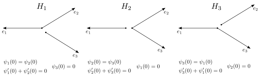
Figure 1: The open graphs depict the Hamiltonians $H_{1}$, $H_{2}$ and $H_{3}$. Under each graph we report the boundary conditions on vectors in the domain of the corresponding Hamiltonian.

With a straightforward computation we have

$$e^{-iH_{j}t}\ =\ U_{t}^{-}\mathbb{I}+U_{t}^{+}{\mathbb{T}}_{j}\,,\qquad t\in\mathbb{R}\,,$$ (2.31)

where ${\mathbb{T}}_{j}$ are the matrices

$${\mathbb{T}}_{1}=\begin{pmatrix}0&1&0\\ 1&0&0\\ 0&0&-1\end{pmatrix}\;;\quad{\mathbb{T}}_{2}=\begin{pmatrix}-1&0&0\\ 0&0&1\\ 0&1&0\end{pmatrix}\;;\quad{\mathbb{T}}_{3}=\begin{pmatrix}0&0&1\\ 0&-1&0\\ 1&0&0\end{pmatrix}\,.$$

2.3 Strichartz’s estimates

A key tool in our method is the extension of the standard Strichartz’s estimates (see e.g. [13]) to the dynamics on $\mathcal{G}$ described by the propagators $e^{-iH_{F}t}$, $e^{-iH_{\delta}^{\alpha}t}$, and $e^{-iH_{\delta^{\prime}}^{\beta}t}$.

In this subsection we use the symbol $H$ to denote any of the three Hamiltonians of interest described in section 2.1.

As a preliminary step, we remark that from equations (2.20), (2.21), (2.22), the standard dispersive estimate immediately follows:

$$\big{\|}e^{-iHt}\Psi\big{\|}_{L^{\infty}}\leqslant\frac{c}{t^{1/2}}\big{\|}\Psi\big{\|}_{L^{1}},\quad t\neq 0\,.$$ (2.32)

Proposition 2.3 (Strichartz Estimates for $e^{-iHt}$).

Let $\Psi_{0}\in L^{2}(\mathcal{G})$, $\Gamma\in L^{q}_{\mathbb{R}}L^{k}$, with $1\leqslant q,k\leqslant 2,\frac{2}{q}+\frac{1}{k}=\frac{5}{2}$, and define

$$\Psi(t)=e^{-iHt}\Psi_{0}\qquad\Phi(t)=\int_{0}^{t}ds\,e^{-iH(t-s)}\Gamma(s)\,.$$

The following estimates hold true:

$$\left\|\Psi\right\|_{L^{p}_{\mathbb{R}}L^{r}}\leqslant c\|\Psi_{0}\|$$ (2.33)

$$\left\|\Phi\right\|_{L^{p}_{\mathbb{R}}L^{r}}\leqslant c\left\|\Gamma\right\|_{L^{q}_{\mathbb{R}}L^{k}}$$ (2.34)

for any pair of indices $(r,p)$ satisfying

$$2\leqslant p,r\leqslant\infty\;,\;\frac{2}{p}+\frac{1}{r}=\frac{1}{2}.$$ (2.35)

The constants $c$ in (2.33) and (2.34) are independent of $T$.

Proof.

The proof is standard due to the dispersive estimate (2.32), see for instance [13] and [19]. ∎

Remark 2.4.

If $H=H^{\alpha}_{\delta}$ ($H^{\beta}_{\delta^{\prime}}$), the constants appearing in (2.32), (2.33) and (2.34) are independent of $\alpha$ ($\beta$). Indeed, by the change of variable $u\to u\alpha$ ($u\to u/\beta$) the integral term in (2.21) ((2.22)) can be easily estimated independently of $\alpha$ ($\beta$), obtaining a dispersive estimate (2.32) independent of the parameters and therefore, by the standard Strichartz machinery, uniform inequalities (2.33) and (2.34).

3 Well-posedness and conservation laws

Here we treat the problem of the well-posedness (in the sense of, e.g., [13]), i.e., the existence and uniqueness of the solution to equation (1.2) in the energy domain of the system. Such a domain turns out to coincide with the form domain of the linear part of equation (1.1). Throughout this section, such a linear part is denoted by $H$, and, according to the particular case under consideration, it can be understood as the Hamiltonian operator $H_{F}$, $H_{\delta}^{\alpha}$, or $H_{\delta^{\prime}}^{\beta}$. Correspondingly, we denote the associated energy domain simply by ${\mathcal{D}}({\mathcal{E}})$. All of the following formulas can be specialized to the particular cases ${\mathcal{D}}({\mathcal{E}}_{F})$, ${\mathcal{D}}({\mathcal{E}}_{\delta}^{\alpha})$, or ${\mathcal{D}}({\mathcal{E}}_{\delta^{\prime}}^{\beta})$.

Let us stress that throughout the paper we do not approximate the dynamics in $H^{1}$, but rather in $L^{2}$. Furthermore, local well-posedness in $L^{2}$ is ensured by Strichartz estimates (proposition 2.3), as is easily seen following the line exposed in [13], chapters 2 and 3. Nonetheless, we prefer to deal with functions in the energy domain, since they are physically more meaningful.

We follow the traditional line of proving, first of all, local well-posedness, and then extending it to all times by means of a priori estimates provided by the conservation laws.

For a more extended treatment of the analogous problem for a two-edge vertex (namely, the real line with a point interaction at the origin), see [3].

First, we endow the energy domain ${\mathcal{D}}({\mathcal{E}})$ with the $H^{1}$-norm defined in (1.5). Second, we denote by ${\mathcal{D}}({\mathcal{E}})^{\star}$ the dual of ${\mathcal{D}}({\mathcal{E}})$, i.e., the set of the continuous linear functionals on ${\mathcal{D}}({\mathcal{E}})$. We denote the dual product of $\Gamma\in{\mathcal{D}}({\mathcal{E}})^{\star}$ and $\Psi\in{\mathcal{D}}({\mathcal{E}})$ by $\langle\Gamma,\Psi\rangle$. In such a bracket we sometimes exchange the place of the factor in ${\mathcal{D}}({\mathcal{E}})^{\star}$ with the place of the factor in ${\mathcal{D}}({\mathcal{E}})$: indeed, the duality product follows the same algebraic rules of the standard scalar product.

As usual, one can extend the action of $H$ to the space ${\mathcal{D}}({\mathcal{E}})$, with values in ${\mathcal{D}}({\mathcal{E}})^{\star}$, by

$$\langle H\Psi_{1},\Psi_{2}\rangle\ :=\ (H^{\frac{1}{2}}\Psi_{1},H^{\frac{1}{2}}\Psi_{2}),$$

where $(\cdot,\cdot)$ denotes the standard scalar product in $L^{2}({\mathcal{G}})$.

Furthermore, for any $\Psi\in{\mathcal{D}}({\mathcal{E}})$ the identity

$$\frac{d}{dt}e^{-iHt}\Psi\ =\ -iHe^{-iHt}\Psi$$ (3.1)

holds in ${\mathcal{D}}({\mathcal{E}})^{\star}$ too. To prove it, one can first test the functional $\frac{d}{dt}e^{-iHt}\Psi$ on an element $\Xi$ in the operator domain ${\mathcal{D}}(H)$, obtaining

$$\left\langle\frac{d}{dt}e^{-iHt}\Psi,\Xi\right\rangle\ =\ \lim_{h\to 0}\left(\Psi,\frac{e^{iH(t+h)}\Xi-e^{iHt}\Xi}{h}\right)\ =\ (\Psi,iHe^{iHt}\Xi)\ =\ \langle-iHe^{-iHt}\Psi,\Xi\rangle.$$

Then, the result can be extended to $\Xi\in{\mathcal{D}}({\mathcal{E}})$ by a density argument.

Besides, by (3.1), the differential version (1.1) of the Schrödinger equation holds in ${\mathcal{D}}({\mathcal{E}})^{\star}$.

In order to prove a well-posedness result we need to generalize standard one-dimensional Gagliardo-Nirenberg estimates to graphs, i.e.

$$\|\Psi\|_{L^{p}}\ \leqslant\ C\|\Psi^{\prime}\|^{\frac{1}{2}-\frac{1}{p}}_{L^{2}}\|\Psi\|^{\frac{1}{2}+\frac{1}{p}}_{L^{2}}\ \qquad+\infty\geqslant p\geqslant 1\ ,$$ (3.2)

where the $C>0$ is a positive constant which depends on the index $p$ only. The proof of (3.2) follows immediately from the analogous estimates for functions of the real line, considering that any function in $H^{1}({\mathbb{R}}^{+})$ can be extended to an even function in $H^{1}({\mathbb{R}})$, and applying this reasoning to each component of $\Psi$.

Proposition 3.1 (Local well-posedness in ${\mathcal{D}}({\mathcal{E}})$).

For any $\Psi_{0}\in{\mathcal{D}}({\mathcal{E}})$, there exists $T>0$ such that the equation (1.2) has a unique solution $\Psi\in C^{0}([0,T),{\mathcal{D}}({\mathcal{E}}))\cap C^{1}([0,T),{\mathcal{D}}({\mathcal{E}})^{\star})$.

Moreover, eq. (1.2) has a maximal solution $\Psi^{\rm{max}}$ defined on an interval of the form $[0,T^{\star})$, and the following “blow-up alternative” holds: either $T^{\star}=\infty$ or

$$\lim_{t\to T^{\star}}\|\Psi_{t}^{\rm{max}}\|_{{\mathcal{D}}({\mathcal{E}})}\ =\ +\infty,$$

where we denoted by $\Psi_{t}^{\rm{max}}$ the function $\Psi^{\rm{max}}$ evaluated at time $t$.

Proof.

We define the space ${\mathcal{X}}:=L^{\infty}([0,T),{\mathcal{D}}({\mathcal{E}})),$ endowed with the norm $\|\Psi\|_{\mathcal{X}}\ :=\ \sup_{t\in[0,T)}\|\Psi_{t}\|_{{\mathcal{D}}({\mathcal{E}})}.$ Given $\Psi_{0}\in{\mathcal{D}}({\mathcal{E}})$, we define the map $G:{\mathcal{X}}\longrightarrow{\mathcal{X}}$ as

$$G\Phi:=e^{-iH\cdot}\Psi_{0}+i\int_{0}^{\cdot}e^{-iH(\cdot-s)}|\Phi_{s}|^{2}\Phi_{s}\,ds.$$

Notice that the nonlinearity preserves the space ${\mathcal{D}}({\mathcal{E}})$. Indeed, since any component $\psi_{i}$ of $\Psi$ belongs to $H^{1}({\mathbb{R}}^{+})$, then $|\psi_{i}|^{2}\psi_{i}$ belongs to $L^{2}({\mathbb{R}}^{+})$ too, and so the energy space for the delta-prime case is preserved. Furthermore, the product preserves the continuity at zero required by the Kirchhoff and the delta case.

By estimates (3.2) one obtains

$$\||\Phi_{s}|^{2}\Phi_{s}\|_{{\mathcal{D}}({\mathcal{E}})}\ \leqslant\ C\|\Phi_{s}\|_{{\mathcal{D}}({\mathcal{E}})}^{3},$$

so

$$\begin{split}\|G\Phi\|_{\mathcal{X}}\ \leqslant\ &\|\Psi_{0}\|_{{\mathcal{D}}({\mathcal{E}})}+C\int_{0}^{T}\|\Phi_{s}\|_{{\mathcal{D}}({\mathcal{E}})}^{3}\,ds\ \leqslant\ \|\Psi_{0}\|_{{\mathcal{D}}({\mathcal{E}})}+CT\|\Phi\|_{\mathcal{X}}^{3}\,.\end{split}$$ (3.3)

Analogously, given $\Phi,\Xi\in{\mathcal{D}}({\mathcal{E}})$,

$$\begin{split}\|G\Phi-G\Xi\|_{\mathcal{X}}\ \leqslant\ &CT\left(\|\Phi\|_{\mathcal{X}}^{2}+\|\Xi\|_{\mathcal{X}}^{2}\right)\|\Phi-\Xi\|_{\mathcal{X}}\,.\end{split}$$ (3.4)

We point out that the constant $C$ appearing in (3.3) and (3.4) is independent of $\Psi_{0}$, $\Phi$, and $\Xi$. Now let us restrict the map $G$ to elements $\Phi$ such that $\|\Phi\|_{\mathcal{X}}\leqslant 2\|\Psi_{0}\|_{{\mathcal{D}}({\mathcal{E}})}$. From (3.3) and (3.4), if $T$ is chosen to be strictly less than $(8C\|\Psi_{0}\|_{{\mathcal{D}}({\mathcal{E}})}^{2})^{-1}$, then $G$ is a contraction of the ball in ${\mathcal{X}}$ of radius $2\|\Psi_{0}\|_{{\mathcal{D}}({\mathcal{E}})}$, and so, by the contraction lemma, there exists a unique solution to (1.2) in the time interval $[0,T)$. By a standard one-step boostrap argument one immediately has that the solution actually belongs to $C^{0}([0,T),{\mathcal{D}}({\mathcal{E}}))$, and due to the validity of (1.1) in the space ${\mathcal{D}}({\mathcal{E}})^{\star}$ we immediately have that the solution $\Psi$ actually belongs to $C^{0}([0,T),{\mathcal{D}}({\mathcal{E}})))\cap C^{1}([0,T),{\mathcal{D}}({\mathcal{E}})^{\star})$.

The proof of the existence of a maximal solution is standard, while the blow-up alternative is a consequence of the fact that, whenever the ${\mathcal{D}}({\mathcal{E}})$-norm of the solution is finite, it is possible to extend it for a further time by the same contraction argument. ∎

The next step consists in the proof of the conservation laws.

Proposition 3.2.

For any solution $\Psi\in C^{0}([0,T),{\mathcal{D}}({\mathcal{E}}))\cap C^{1}([0,T),{\mathcal{D}}({\mathcal{E}})^{\star})$ to the problem (1.2), the following conservation laws hold at any time $t$:

$$\|\Psi_{t}\|\ =\ \|\Psi_{0}\|,\qquad{\mathcal{E}}(\Psi_{t})\ =\ {\mathcal{E}}(\Psi_{0}),$$

where the symbol ${\mathcal{E}}$ denotes the energy functional

$${\mathcal{E}}(\Psi_{t})\ :=\ \frac{1}{2}{\mathcal{E}}_{lin}(\Psi_{t})-\frac{1}{4}\|\Psi_{t}\|_{L^{4}}^{4}.$$

Here the functional ${\mathcal{E}}_{lin}$ coincides with ${\mathcal{E}}_{F}$, ${\mathcal{E}}_{\delta}^{\alpha}$ or ${\mathcal{E}}_{\delta^{\prime}}^{\beta}$, according to the case one considers.

Proof.

The conservation of the $L^{2}$-norm can be immediately obtained by the validity of equation (1.1) in the space ${\mathcal{D}}({\mathcal{E}})$:

$$\frac{d}{dt}\|\Psi_{t}\|^{2}\ =\ 2\,{\rm{Re}}\,\left\langle\Psi_{t},\frac{d}{dt}\Psi_{t}\right\rangle\ =\ 2\,{\rm{Im}}\,\langle\Psi_{t},H\Psi_{t}\rangle\ =\ 0$$

by the self-adjointness of $H$. In order to prove the conservation of the energy, first we notice that $\langle\Psi_{t},H\Psi_{t}\rangle$ is differentiable as a function of time. Indeed,

$$\begin{split}&\frac{1}{h}\left[\langle\Psi_{t+h},H\Psi_{t+h}\rangle-\langle\Psi_{t},H\Psi_{t}\rangle\right]\ =\ \left\langle\frac{\Psi_{t+h}-\Psi_{t}}{h},H\Psi_{t+h}\right\rangle+\left\langle H\Psi_{t},\frac{\Psi_{t+h}-\Psi_{t}}{h}\right\rangle\end{split}$$

and then, passing to the limit $h\to 0$,

$$\frac{d}{dt}(\Psi_{t},H\Psi_{t})\ =\ 2\,{\rm{Re}}\,\left\langle\frac{d}{dt}\Psi_{t},H\Psi_{t}\right\rangle\ =\ 2\,{\rm{Im}}\,\langle|\Psi_{t}|^{2}\Psi_{t},H\Psi_{t}\rangle,$$ (3.5)

where we used the self-adjointness of $H$ and (1.1). Furthermore,

$$\frac{d}{dt}(\Psi_{t},|\Psi_{t}|^{2}\Psi_{t})\ =\ \frac{d}{dt}(\Psi_{t}^{2},\Psi_{t}^{2})\ =\ 4\,{\rm{Im}}\,\langle|\Psi_{t}|^{2}\Psi_{t},H\Psi_{t}\rangle.$$ (3.6)

From (3.5) and (3.6) one then obtains

$$\frac{d}{dt}{\mathcal{E}}(\Psi_{t})\ =\ \frac{1}{2}\frac{d}{dt}\langle\Psi_{t},H\Psi_{t}\rangle-\frac{1}{4}\frac{d}{dt}(\Psi_{t},|\Psi_{t}|^{2}\Psi_{t})_{L^{2}}\ =\ 0$$

and the proposition is proved. ∎

Corollary 3.3.

The solutions are globally defined in time.

Proof.

By estimate (3.2) with $p=\infty$ and conservation of the $L^{2}$-norm, there exists a constant $M$, that depends on $\Psi_{0}$ only, such that

$${\mathcal{E}}(\Psi_{0})\ =\ {\mathcal{E}}(\Psi_{t})\ \geq\ \frac{1}{2}\|\Psi_{t}^{\prime}\|^{2}-M\|\Psi_{t}^{\prime}\|$$

Therefore a uniform (in $t$) bound on $\|\Psi_{t}^{\prime}\|^{2}$ is obtained. As a consequence, one has that no blow-up in finite time can occur, and therefore, by the blow-up alternative, the solution is global in time. ∎

4 Main Result

In this section we describe the asymptotic dynamics of a particular initial state, which resembles a soliton for the standard cubic NLS on the line.

According to section 3, we use the symbol $H$ to generically denote the linear part of the evolution, regardless of the fact that we are considering the Kirchhoff, delta, or delta-prime boundary conditions. When necessary, we will distinguish between the three of them.

We use the notation

$$\phi(x)\ =\ \sqrt{2}\cosh^{-1}x\,,\quad x\in\mathbb{R}\,,$$

and for any $x_{0}\in\mathbb{R}$ and $v\in\mathbb{R}$ we define

$$\phi_{x_{0},v}(x,t)=e^{i\frac{v}{2}x}{e^{-it\frac{v^{2}}{4}}}e^{it}\phi(x-x_{0}-vt)\,,\quad x\in\mathbb{R},\ t\in\mathbb{R}\,.$$ (4.1)

The function $\phi_{x_{0},v}$ represents a soliton for the cubic NLS on the line which at time $t=0$ is centered in $x=x_{0}$ and has velocity $v$. Therefore, $\phi_{x_{0},v}$ is the solution of the integral equation

$$\phi_{x_{0},v}(x,t)=\big{[}U_{t}e^{i\frac{v}{2}\cdot}\phi(\cdot-x_{0})\big{]}(x)+i\int_{0}^{t}\big{[}U_{t-s}|\phi_{x_{0},v}(\cdot,s)|^{2}\phi_{x_{0},v}(\cdot,s)\big{]}(x)ds\,,\quad t\in\mathbb{R}\,.$$ (4.2)

Let $\chi$ be the cut off function $\chi\in C^{\infty}({\mathbb{R}}^{+})$, $\chi=1$ in $(2,+\infty)$ and $\chi=0$ in $(0,1)$. For later use we define also $\chi_{+}=\chi_{[0,+\infty)}$ and $\chi_{-}=\chi_{(-\infty,0]}$, where $\chi_{[a,b]}$ denotes the characteristic function of the interval $[a,b]$.

Moreover let $x_{0}$ and $v$ be two positive constants and $0<\delta<1$.

We take as initial condition the following function

$$\Psi_{0}(x)\ =\ \left(\begin{array}[]{c}\chi(x)e^{-i\frac{v}{2}x}\phi(x-x_{0})\\ 0\\ 0\end{array}\right)\,,\qquad x_{0}\ \geqslant\ v^{1-\delta}\,,$$ (4.3)

and we denote by $\Psi_{H,t}$ the solution of the equation

$$\Psi_{H,t}\ =\ e^{-iHt}\Psi_{0}+i\int_{0}^{t}ds\,e^{-iH(t-s)}|\Psi_{H,s}|^{2}\Psi_{H,s}\,,\quad t\geqslant 0\,.$$ (4.4)

The choice of the vector $\Psi_{0}$ is used to render the idea that the initial condition is a soliton centered away from the vertex and moving towards the vertex with velocity $v$. The cut off function $\chi$ in formula (4.3) is aimed at setting $\Psi_{0}$ in the domain of the Hamiltonian $H$, see section 2.1.

Let us set $t_{2}:=x_{0}/v+v^{-\delta}$ and define the following functions:

$$\Phi^{1}_{H,t_{2}}(x_{1},x_{2},x_{3})\equiv\begin{pmatrix}\tilde{r}_{H}e^{-i\frac{v^{2}}{4}t_{2}}e^{i\frac{v}{2}x_{1}}e^{it_{2}}\phi(x_{1}+x_{0}-vt_{2})\\ \tilde{r}_{H}e^{-i\frac{v^{2}}{4}t_{2}}e^{-i\frac{v}{2}x_{2}}e^{it_{2}}\phi(x_{2}-x_{0}+vt_{2})\\ 0\end{pmatrix}$$ (4.5)

$$\Phi^{2}_{H,t_{2}}(x_{1},x_{2},x_{3})\equiv\begin{pmatrix}0\\ \tilde{t}_{H}e^{-i\frac{v^{2}}{4}t_{2}}e^{i\frac{v}{2}x_{2}}e^{it_{2}}\phi(x_{2}+x_{0}-vt_{2})\\ \tilde{t}_{H}e^{-i\frac{v^{2}}{4}t_{2}}e^{-i\frac{v}{2}x_{3}}e^{it_{2}}\phi(x_{3}-x_{0}+vt_{2})\end{pmatrix}$$ (4.6)

$$\Phi^{3}_{H,t_{2}}(x_{1},x_{2},x_{3})\equiv\begin{pmatrix}\tilde{t}_{H}e^{-i\frac{v^{2}}{4}t_{2}}e^{-i\frac{v}{2}x_{1}}e^{it_{2}}\phi(x_{1}-x_{0}+vt_{2})\\ 0\\ \tilde{t}_{H}e^{-i\frac{v^{2}}{4}t_{2}}e^{i\frac{v}{2}x_{3}}e^{it_{2}}\phi(x_{3}+x_{0}-vt_{2})\end{pmatrix}$$ (4.7)

They represent solitons on the line multiplied by the scattering coefficients of the linear dynamics $\tilde{r}_{H}$ and $\tilde{t}_{H}$, that, in the particular regime we consider, are defined as follows:

$$\begin{split}&\tilde{r}_{H_{F}}\ =\ -1/3,\qquad\tilde{t}_{H_{F}}\ =\ 2/3\\ &\tilde{r}_{H_{\delta}^{\tilde{\alpha}v}}\ =\ -\frac{1+2i\tilde{\alpha}}{3+2i\tilde{\alpha}},\qquad\tilde{t}_{H_{\delta}^{\tilde{\alpha}v}}\ =\ \frac{2}{3+2i\tilde{\alpha}}\\ &\tilde{r}_{H_{\delta^{\prime}}^{\tilde{\beta}/v}}\ =\ \frac{\tilde{\beta}+2i}{\tilde{\beta}+6i},\qquad\tilde{t}_{H_{\delta^{\prime}}^{\tilde{\beta}/v}}\ =\ -\frac{4i}{\tilde{\beta}+6i}\,.\end{split}$$ (4.8)

Remark 4.1.

Notice that the coefficients $\tilde{r}_{H}$ and $\tilde{t}_{H}$ can be obtained by the scattering coefficients (2.29), (2.30), identifying $k$ with $v/2$ and replacing $\alpha$ by $\tilde{\alpha}v$ and $\beta$ by $\tilde{\beta}/v$. This is due to the fact that we implicitly considered a particle with mass equal to $1/2$, therefore the momentum $k$ is linked to the speed $v$ by $k=v/2$.

For any $t>t_{2}$ we define the vectors $\Phi^{j}_{H,t}$ as the evolution of $\Phi^{j}_{H,t_{2}}$ with the nonlinear flow generated by $H_{j}$, i.e., they are solutions of the equation

$$\Phi^{j}_{H,t}=e^{-iH_{j}(t-t_{2})}\Phi^{j}_{H,t_{2}}+i\int_{t_{2}}^{t}ds\,e^{-iH_{j}(t-s)}|\Phi^{j}_{H,s}|^{2}\Phi^{j}_{H,s}\qquad j=1,2,3\,.$$ (4.9)

Remark 4.2.

The vectors $\Phi^{j}_{H,t}$ can be represented by

$$\Phi^{1}_{H,t}(x_{1},x_{2},x_{3})=\begin{pmatrix}e^{-i\frac{v^{2}}{4}t_{2}}e^{it_{2}}\phi^{ref}_{t-t_{2}}(x_{1})\\ e^{-i\frac{v^{2}}{4}t_{2}}e^{it_{2}}\phi^{ref}_{t-t_{2}}(-x_{2})\\ 0\end{pmatrix}\;;\quad\Phi^{2}_{H,t}(x_{1},x_{2},x_{3})=\begin{pmatrix}0\\ e^{-i\frac{v^{2}}{4}t_{2}}e^{it_{2}}\phi^{tr}_{t-t_{2}}(x_{2})\\ e^{-i\frac{v^{2}}{4}t_{2}}e^{it_{2}}\phi^{tr}_{t-t_{2}}(-x_{3})\end{pmatrix}$$ (4.10)

$$\Phi^{3}_{H,t}(x_{1},x_{2},x_{3})=\begin{pmatrix}e^{-i\frac{v^{2}}{4}t_{2}}e^{it_{2}}\phi^{tr}_{t-t_{2}}(-x_{1})\\ 0\\ e^{-i\frac{v^{2}}{4}t_{2}}e^{it_{2}}\phi^{tr}_{t-t_{2}}(x_{3})\end{pmatrix}\,$$ (4.11)

where, for any $t\geqslant 0$, the functions $\phi^{ref}_{t}$ and $\phi^{tr}_{t}$ are the solutions to the following NLS on the line

$$\phi^{ref}_{t}(x)=\tilde{r}_{H}\int_{-\infty}^{\infty}U_{t}(x-y)e^{i\frac{v}{2}y}\phi(y-v^{1-\delta})dy+i\int_{0}^{t}ds\int_{-\infty}^{\infty}U_{t-s}(x-y)|\phi^{ref}_{s}(y)|^{2}\phi^{ref}_{s}(y)dy$$ (4.12)

$$\phi^{tr}_{t}(x)=\tilde{t}_{H}\int_{-\infty}^{\infty}U_{t}(x-y)e^{i\frac{v}{2}y}\phi(y-v^{1-\delta})dy+i\int_{0}^{t}ds\int_{-\infty}^{\infty}U_{t-s}(x-y)|\phi^{tr}_{s}(y)|^{2}\phi^{tr}_{s}(y)dy\,.$$ (4.13)

Our main result is summarized in the following theorem:

Theorem 4.3.

Fixed $\tilde{\alpha},\tilde{\beta}>0$, let $H$ be any of the self-adjoint operators $H_{F}$, $H_{\delta}^{\tilde{\alpha}v}$, $H_{\delta^{\prime}}^{\tilde{\beta}/v}$ acting on $L^{2}(\mathcal{G})$, where ${\mathcal{G}}$ is the three-edge star graph, and defined by (2.1), (2.2), (2.3), (2.4). Call $\Psi_{t}$ the unique, global solution to the Cauchy problem (4.4) with initial data (4.3).

Then, there exist $\tau_{*}>0$ and $T_{\ast}>0$ such that for $0<T<T_{\ast}$ one has

$$\|\Psi_{t}-\Phi^{1}_{t}-\Phi^{2}_{t}-\Phi^{3}_{t}\|_{L_{x}^{2}(\mathcal{G})}\ \leqslant\ Cv^{-\frac{T_{\ast}-T}{\tau_{*}}}$$ (4.14)

for any time $t$ in the interval $x_{0}/v+v^{1-\delta}<t<x_{0}/v+v^{1-\delta}+T\ln v$.

In (4.14), $C$ is a positive constant independent of $t$ and $v$, the functions $\Phi_{t}^{j}$ are defined by formulas (1.4), $\tilde{t}$ and $\tilde{r}$, given in (4.8), are the scattering coefficients associated to $H$.

The proof of the theorem will be broken into three steps or equivalently we break the time evolution of $\Psi_{H,t}$ into three phases.

Remark 4.4.

A further consequence of Theorem 4.3, as in the case of [17], is the fact that fast solitons have reflection and transmission coefficients which, up to negligible corrections, coincide with the corresponding coefficients of the linear graph. For example, a definition of the transmission coefficients along the branches $j=2,3$ could be given considering the ratio between the amount of mass on the $j-$edge and the total mass, in the limit $t\to\infty$:

$$\lim_{t\to\infty}\frac{\|\Psi^{j}_{t}\|}{\|\Psi_{t}\|}\equiv|t^{j}(v)|\ ,$$

where $\Psi^{j}$ denotes the restriction of the solution to the $j-$edge. In our case we do not have at our disposal the rigorous asymptotics for $t\to\infty$; nevertheless, we can obtain a weaker result. We have the results of Theorem 1.1, which give, in the time interval $t_{2}<t<t_{2}+T\ln v\ ,$ the estimate

$$\frac{\|\Psi^{j}_{t}\|}{\|\Psi_{t}\|}=|\tilde{t}^{j}|+{\mathcal{O}}(v^{-\sigma})$$

for a certain $\sigma>0$ and where $\tilde{t}^{j}$ is the scattering coefficient of the linear Hamiltonian which describes the vertex. So, in the limit of fast solitons, i.e. $v\to\infty$, one can assert that the ratio which defines the nonlinear scattering coefficient converges to the corresponding linear scattering coefficient. And analogously for the case of reflection coefficient $r(v)$, i.e. $j=1$, one has (for $t>t_{2}$, as before)

$$\lim_{v\to\infty}\frac{\|\Psi^{1}_{t}\|}{\|\Psi_{t}\|}=|\tilde{r}|\ .$$

This is true for every coupling between the ones considered, i.e. Kirchhoff, $\delta$ or $\delta^{\prime}$.

5 Proof of theorem 4.3

In the proof we drop the subscript $H$. When convenient, we specify the particular Hamiltonian operator we refer to.

For any $t\in\mathbb{R}$ we introduce the soliton

$$\Phi_{t}(x_{1},x_{2},x_{3})\ =\ \left(\begin{array}[]{c}e^{-i\frac{v^{2}}{4}t}e^{-i\frac{v}{2}x_{1}}e^{it}\phi(x_{1}-x_{0}+vt)\\ e^{-i\frac{v^{2}}{4}t}e^{i\frac{v}{2}x_{2}}e^{it}\phi(x_{2}+x_{0}-vt)\\ 0\end{array}\right)\,.$$ (5.1)

Then, the function $\Phi_{t}$ satisfies the equation

$$\Phi_{t}\ =\ e^{-iH_{1}t}\Phi_{0}+i\int_{0}^{t}ds\,e^{-iH_{1}(t-s)}|\Phi_{s}|^{2}\Phi_{s}\,,\quad t\geqslant 0\,.$$ (5.2)

5.1 Phase 1

We call “phase 1” the dynamics in the time interval $\left(0,t_{1}\right)$ with $t_{1}=\frac{x_{0}}{v}-v^{-\delta}$. In this interval we approximate the solution by the soliton (5.1). The content of this subsection is the estimate of the error due to such an approximation, that is contained in proposition 5.3. Before proving it, we need two lemmas.

Lemma 5.1.

Given $0\leqslant t_{a}\leqslant t_{b}\leqslant t_{1}$, for the functions

$$\begin{split}K_{1}(t,x)&\ :=\ \int_{0}^{\infty}U_{t-t_{a}}(x+y)e^{-i\frac{v}{2}y}\phi(y-x_{0})\,dy+i\int_{t_{a}}^{t}ds\int_{0}^{\infty}U_{t-s}(x+y)e^{-i\frac{v}{2}y}{e^{-is\frac{v^{2}}{4}}}e^{is}\phi^{3}(y-x_{0}+vs)\,dy\\ K_{2}(t,x)&\ :=\ \int_{0}^{\infty}U_{t-t_{a}}(x+y)e^{i\frac{v}{2}y}\phi(y+x_{0})\,dy+i\int_{t_{a}}^{t}ds\int_{0}^{\infty}U_{t-s}(x+y)e^{i\frac{v}{2}y}{e^{-is\frac{v^{2}}{4}}}e^{is}\phi^{3}(y+x_{0}-vs)\,dy\end{split}$$ (5.3)

the following estimate holds:

$$\|K_{i}\|_{X_{t_{a},t_{b}}({\mathbb{R}}^{+})}\leqslant\ Ce^{-x_{0}+vt_{b}},\qquad i=1,2,$$

where $X_{t_{a},t_{b}}({\mathbb{R}}^{+}):=L^{\infty}_{[t_{a},t_{b}]}L^{2}({\mathbb{R}}^{+})\cap L^{6}_{[t_{a},t_{b}]}L^{6}({\mathbb{R}}^{+})$.

Proof.

Let us start with $K_{1}$. Adding and subtracting a contribution to negative values of $y$ one can write

$$\begin{split}K_{1}(t,x)&\ =\ \int_{-\infty}^{\infty}U_{t-t_{a}}(x+y)e^{-i\frac{v}{2}y}\phi(y-x_{0})\,dy+i\int_{t_{a}}^{t}ds\int_{-\infty}^{\infty}U_{t-s}(x+y)e^{-i\frac{v}{2}y}{e^{-is\frac{v^{2}}{4}}}e^{is}\phi^{3}(y-x_{0}+vs)\,dy\\ &\ -\int_{-\infty}^{0}U_{t-t_{a}}(x+y)e^{-i\frac{v}{2}y}\phi(y-x_{0})\,dy-i\int_{t_{a}}^{t}ds\int_{-\infty}^{0}U_{t-s}(x+y)e^{-i\frac{v}{2}y}{e^{-is\frac{v^{2}}{4}}}e^{is}\phi^{3}(y-x_{0}+vs)\,dy\\ =&\ e^{i\frac{v}{2}x}{e^{-it\frac{v^{2}}{4}}}e^{it}\phi(x+x_{0}-vt)\\ &\ -\int_{-\infty}^{0}U_{t-t_{a}}(x+y)e^{-i\frac{v}{2}y}\phi(y-x_{0})\,dy-i\int_{t_{a}}^{t}ds\int_{-\infty}^{0}U_{t-s}(x+y)e^{-i\frac{v}{2}y}{e^{-is\frac{v^{2}}{4}}}e^{is}\phi^{3}(y-x_{0}+vs)\,dy\end{split}$$ (5.4)

where we used the integral equation (4.2). By a straightforward computation, the $X_{t_{a},t_{b}}({\mathbb{R}}^{+})$-norm of the first term can be bounded by $Ce^{-(x_{0}-vt_{b})}.$ To evaluate the size of the second term, let us write it as follows:

$$\int_{0}^{\infty}U_{t-t_{a}}(x-y)e^{i\frac{v}{2}y}\phi(y+x_{0})dy\ =[U^{-}_{t-t_{a}}e^{i\frac{v}{2}\cdot}\phi(\cdot+x_{0})](x)=\ [U_{t-t_{a}}\chi_{+}e^{i\frac{v}{2}\cdot}\phi(\cdot+x_{0})](x),\quad x>0.$$ (5.5)

Using the one-dimensional homogeneous Strichartz’s estimates for $U_{t-t_{a}}$, namely, the analogous of (2.33) for functions of the half line, we can estimate the $X_{t_{a},t_{b}}(\mathbb{R}^{+})$-norm of this term as

$$\|U_{t-t_{a}}\chi_{+}e^{i\frac{v}{2}\cdot}\phi(\cdot+x_{0})\|_{X_{t_{a},t_{b}}(\mathbb{R})}\leqslant C\|\chi_{+}e^{i\frac{v}{2}\cdot}\phi(\cdot+x_{0})\|\ \leqslant Ce^{-x_{0}},$$

where we used the notation $X_{t_{a},t_{b}}({\mathbb{R}}):=L^{\infty}_{[t_{a},t_{b}]}L^{2}({\mathbb{R}})\cap L^{6}_{[t_{a},t_{b}]}L^{6}({\mathbb{R}})$.

The norm of the last term on the r.h.s. of equation (5.4) can be estimated in a similar way by

$$\left\|\int_{t_{a}}^{\cdot}\big{[}U_{\cdot-s}|\phi_{-x_{0},v}(s)|^{2}\phi_{-x_{0},v}(s)\big{]}ds\right\|_{X_{t_{a},t_{b}}(\mathbb{R}^{+})}\ \leqslant C\|\phi_{-x_{0},v}^{3}\|_{L^{1}_{[t_{a},t_{b}]}L^{2}(\mathbb{R}^{+})}\leqslant C\frac{1}{v}e^{-x_{0}+vt_{b}}.$$ (5.6)

Therefore, from (5.4), (5.5), and (5.6) we get

$$\|K_{1}\|_{X_{t_{a},t_{b}}({\mathbb{R}}^{+})}\ \leqslant\ Ce^{-x_{0}+vt_{b}}.$$

To estimate $K_{2}$, the first term in its definition (5.3) can be treated as in (5.5), while the second is estimated following the line of (5.6). ∎

Lemma 5.2.

Given $0\leqslant t_{a}\leqslant t_{b}\leqslant t_{1}$, let $a$ and $b$ two strictly positive numbers, with

$$b\leqslant\frac{1}{8a^{2}+4a}.$$

Moreover, let $y$ be a real, continuous function such that $0\leqslant y(t_{a})\leqslant a$, and

$$0\leqslant y(t)\leqslant a+by^{2}(t)+by^{3}(t),\qquad{\mbox{for any }}\ t\in[t_{a},t_{b}].$$ (5.7)

Then,

$$\max_{t\in[t_{a},t_{b}]}y(t)\,\leqslant\,2a.$$

Proof.

Consider the function $f_{b}(x):=bx^{3}+bx^{2}-x+a$. Denoted $\bar{b}:=\frac{1}{8a^{2}+4a}$, one has $f_{\bar{b}}(2a)\ =0$.

If $b\leqslant\bar{b}$, then $f_{b}(x)\leqslant f_{\bar{b}}(x)$ for any $x>0$. Besides, notice that $f_{b}(0)=a>0$, then there must be a point $\tilde{x}\in(0,2a]$ s.t. $f_{b}(\tilde{x})=0$. Finally, since the function $y$ is continuous, in order to satisfy the constraint (5.7) one must have

$$y(t)\leqslant\tilde{x}\leqslant 2a,\qquad{\mbox{for any }}\ t\in[t_{a},t_{b}].$$

∎

Proposition 5.3.

Let $\Psi_{t}$ be the solution of the equation (4.4), and $\Phi_{t}$ be the solution of equation (5.2). There exists $C>0$, independent of $t$ and $v$, such that

$$\|\Psi_{t}-\Phi_{t}\|\ \leqslant\ Ce^{-v^{1-\delta}}$$ (5.8)

for any $t\in[0,t_{1}]$.

Proof.

Let us define $\Xi_{t}:=\Psi_{t}-\Phi_{t}$, and fix $t_{a}\in[0,t_{1}]$. Then, from equations (4.4) and (5.2), we have

$$\begin{split}\Xi_{t}\ =&\ e^{-iH(t-t_{a})}\Xi_{t_{a}}+(e^{-iH(t-t_{a})}-e^{-iH_{1}(t-t_{a})})\Phi_{t_{a}}+i\int_{t_{a}}^{t}(e^{-iH(t-s)}-e^{-iH_{1}(t-s)})|\Phi_{s}|^{2}\Phi_{s}\,ds\\ &\ +i\int_{t_{a}}^{t}e^{-iH(t-s)}\left[|\Xi_{s}|^{2}\Xi_{s}+|\Xi_{s}|^{2}\Phi_{s}+|\Phi_{s}|^{2}\Xi_{s}+2{\mbox{Re}}(\overline{\Xi_{s}}\Phi_{s})\Xi_{s}+2{\mbox{Re}}(\overline{\Xi_{s}}\Phi_{s})\Phi_{s}\right]\\ =&\ e^{-iH(t-t_{a})}\Xi_{t_{a}}+F(t_{a},t)\\ &+i\int_{t_{a}}^{t}e^{-iH(t-s)}\left[|\Xi_{s}|^{2}\Xi_{s}+|\Xi_{s}|^{2}\Phi_{s}+|\Phi_{s}|^{2}\Xi_{s}+2{\mbox{Re}}(\overline{\Xi_{s}}\Phi_{s})\Xi_{s}+2{\mbox{Re}}(\overline{\Xi_{s}}\Phi_{s})\Phi_{s}\right],\end{split}$$

where we defined

$$F(t_{a},t)\ :=\ (e^{-iH(t-t_{a})}-e^{-iH_{1}(t-t_{a})})\Phi_{t_{a}}+i\int_{t_{a}}^{t}(e^{-iH(t-s)}-e^{-iH_{1}(t-s)})|\Phi_{s}|^{2}\Phi_{s}\,ds\,.$$

Let us fix $t_{b}\in[t_{a},t_{1}]$, and denote $X_{t_{a},t_{b}}=L^{\infty}_{[t_{a},t_{b}]}L^{2}\cap L^{6}_{[t_{a},t_{b}]}L^{6}$. Then

$$\begin{split}\|\Xi\|_{X_{t_{a},t_{b}}}\ \leqslant&\ \|e^{-iH(\cdot-t_{a})}\Xi_{t_{a}}\|_{X_{t_{a},t_{b}}}+\|F(t_{a},\cdot)\|_{X_{t_{a},t_{b}}}\\ &+\left\|\int_{t_{a}}^{\cdot}e^{-iH(\cdot-s)}\left[|\Xi_{s}|^{2}\Xi_{s}+|\Xi_{s}|^{2}\Phi_{s}+|\Phi_{s}|^{2}\Xi_{s}+2{\mbox{Re}}(\overline{\Xi_{s}}\Phi_{s})\Xi_{s}+2{\mbox{Re}}(\overline{\Xi_{s}}\Phi_{s})\Phi_{s}\right]\right\|_{X_{t_{a},t_{b}}}.\end{split}$$ (5.9)

Using (2.33) the first term on the r.h.s can be estimated as

$$\|e^{-iH(\cdot-t_{a})}\Xi_{t_{a}}\|_{X_{t_{a},t_{b}}}\ \leqslant\ C\|\Xi_{t_{a}}\|.$$

We estimate the integral term on the r.h.s. of (5.9) also using Strichartz’s estimates. Let us analyse in detail the cubic term. Since both pairs of indices $(\infty,2)$ and $(6,6)$ fulfil (2.35), in (2.34) we can choose $q=k=6/5$ and obtain

$$\left\|\int_{t_{a}}^{\cdot}e^{-iH(\cdot-s)}|\Xi_{s}|^{2}\Xi_{s}\,ds\right\|_{X_{t_{a},t_{b}}}\leqslant C\||\Xi_{\cdot}|^{2}\Xi_{\cdot}\|_{L^{6/5}_{[t_{a},t_{b}]}L^{6/5}}.$$ (5.10)

Moreover, by standard Hölder estimates,

$$\||\Xi_{\cdot}|^{2}\Xi_{\cdot}\|_{L^{6/5}_{[t_{a},t_{b}]}L^{6/5}}\ \leqslant\ \left\|\|\Xi_{\cdot}\|^{2}_{L^{6}}\|\Xi_{\cdot}\|_{L^{2}}\right\|_{L^{6/5}_{[t_{a},t_{b}]}}\ \leqslant\ \|\Xi\|^{2}_{L^{6}_{[t_{a},t_{b}]}L^{6}}\|\Xi\|_{L^{2}_{[t_{a},t_{b}]}L^{2}}\ \leqslant\ (t_{b}-t_{a})^{\frac{1}{2}}\|\Xi\|^{2}_{L^{6}_{[t_{a},t_{b}]}L^{6}}\|\Xi\|_{L^{\infty}_{[t_{a},t_{b}]}L^{2}}.$$ (5.11)

Then, by (5.10) and (5.11),

$$\left\|\int_{t_{a}}^{\cdot}e^{-iH(\cdot-s)}|\Xi_{s}|^{2}\Xi_{s}\,ds\right\|_{X_{t_{a},t_{b}}}\leqslant C(t_{b}-t_{a})^{1/2}\|\Xi\|^{3}_{X_{t_{a},t_{b}}}.$$ (5.12)

Notice that the constant $C$ can be chosen independently of $t_{a},t_{b}$, and of the boundary condition at the vertex.

The other terms in the integral on the r.h.s. of (5.9) can be estimated analogously. One ends up with

$$\begin{split}\|\Xi\|_{X_{t_{a},t_{b}}}\leqslant&\ C\ \|\Xi_{t_{a}}\|+\|F(t_{a},\cdot)\|_{X_{t_{a},t_{b}}}+C(t_{b}-t_{a})^{\frac{1}{2}}\|\Xi\|^{3}_{X_{t_{a},t_{b}}}+C(t_{b}-t_{a})^{\frac{2}{3}}\|\Xi\|^{2}_{X_{t_{a},t_{b}}}+C(t_{b}-t_{a})^{\frac{5}{6}}\|\Xi\|_{X_{t_{a},t_{b}}},\end{split}$$

where the arising norms of $\Phi$ were absorbed in the constant $C$.

If $t_{b}$ and $t_{a}$ are sufficiently close, then $C(t_{b}-t_{a})^{\frac{5}{6}}<1/2$. Furthermore, since the quantity $t_{b}-t_{a}$ is upper bounded, one can estimate $(t_{b}-t_{a})^{\frac{2}{3}}$ by $C(t_{b}-t_{a})^{\frac{1}{2}}$. So, for some $\widetilde{C}>0$

$$\begin{split}\|\Xi\|_{X_{t_{a},t_{b}}}\leqslant&\ \widetilde{C}\ \|\Xi_{t_{a}}\|+\widetilde{C}\ \|F(t_{a},\cdot)\|_{X_{t_{a},t_{b}}}+\widetilde{C}(t_{b}-t_{a})^{\frac{1}{2}}\left[\|\Xi\|^{3}_{X_{t_{a},t_{b}}}+\|\Xi\|^{2}_{X_{t_{a},t_{b}}}\right].\end{split}$$ (5.13)

Applying lemma 5.2 to the function $y(t)=\|\Xi\|_{X_{t_{a},t}}$, which is continuous and monotone, one has that, if

$$t_{b}-t_{a}\ \leqslant\ \left(8\widetilde{C}^{3}\ (\ \|\Xi_{t_{a}}\|+\|F(t_{a},\cdot)\|_{X_{t_{a},t_{b}}})^{2}+4\widetilde{C}^{2}\ (\|\Xi_{t_{a}}\|+\|F(t_{a},\cdot)\|_{X_{t_{a},t_{b}}})\right)^{-2},$$

then $\|\Xi\|_{X_{t_{a},t_{b}}}\leqslant\ 2\widetilde{C}\ \|\Xi_{t_{a}}\|+2\widetilde{C}\ \|F(t_{a},\cdot)\|_{X_{t_{a},t_{b}}}$. From the immediate estimates

$$\|\Xi_{t_{a}}\|\ \leqslant\ 4,\qquad\|F(t_{a},\cdot)\|_{X_{t_{a},t_{b}}}\ \leqslant\ \|F(0,\cdot)\|_{X_{0,t_{1}}},$$

if one denotes

$$\tau\ :=\ \left(8\widetilde{C}^{3}\ (4+\|F(t_{a},\cdot)\|_{X_{0,t_{1}}})^{2}+4\widetilde{C}^{2}\ (4+\|F(t_{a},\cdot)\|_{X_{0,t_{1}}})\right)^{-2},$$

then for any $t\in[0,t_{1})$ $\|\Xi\|_{X_{t,t+\tau}}\leqslant\ 2\widetilde{C}\ \|\Xi_{t}\|+2\widetilde{C}\ \|F(t,\cdot)\|_{X_{t,t+\tau}}$.

We divide the interval $[0,t_{1}]$ in $N+1$ subintervals as follows

$$[0,t_{1}]\ =\ \left(\cup_{j=0}^{N-1}[j\tau,(j+1)\tau]\right)\cup[N\tau,t_{1}],$$

where

$$N:=\left[\frac{x_{0}-v^{1-\delta}}{v\tau}\right],\qquad[\cdot]={\mbox{ integer part.}}$$

Making use of lemma 5.2, and noting that $\|\Xi_{(j+1)\tau}\|\leqslant\|\Xi\|_{X_{j\tau,(j+1)\tau}}$, one proves by induction that

$$\begin{split}\|\Xi\|_{X_{j\tau,(j+1)\tau}}\ &\leqslant\ (2\widetilde{C})^{j+1}\|\Xi_{0}\|+\sum_{k=0}^{j}(2\widetilde{C})^{j+1-k}\|F(k\tau,\cdot)\|_{X_{k\tau,(k+1)\tau}},\qquad j=0,\dots,N-1,\\ \|\Xi\|_{X_{N\tau,t_{1}}}\ &\leqslant\ (2\widetilde{C})^{N+1}\|\Xi_{0}\|+\sum_{k=0}^{N-1}(2\widetilde{C})^{N+1-k}\|F(k\tau,\cdot)\|_{X_{k\tau,(k+1)\tau}}+2\widetilde{C}\ \|F(N\tau,\cdot)\|_{X_{N\tau,t_{1}}}\,,\end{split}$$ (5.14)

where the last inequality comes from the fact that $t_{1}-N\tau\leqslant\tau$, so lemma 5.2 applies to this last step too.

The norm of $\Xi$ as a function of the whole time interval $[0,t_{1}]$ can be estimated by

$$\begin{split}\|\Xi\|_{X_{0,t_{1}}}\ \leqslant&\ \sum_{j=0}^{N-1}\|\Xi\|_{X_{j\tau,(j+1)\tau}}+\|\Xi\|_{X_{N\tau,t_{1}}}\\ \leqslant&\ \sum_{j=0}^{N}(2\widetilde{C})^{j+1}\|\Xi_{0}\|+\sum_{j=0}^{N}\sum_{k=0}^{j}(2\widetilde{C})^{j+1-k}\|F(k\tau,\cdot)\|_{X_{k\tau,\min\{t_{1},(k+1)\tau\}}}\,.\end{split}$$ (5.15)

In order to prove the theorem using (5.15), we need more precise estimates for $\|\Xi_{0}\|$ and $\|F(j\tau,\cdot)\|_{X_{j\tau,(j+1)\tau}}$.

First,

$$\|\Xi_{0}\|^{2}\leqslant\ \int_{0}^{2}\phi^{2}(x-x_{0})\,dx+\int_{0}^{\infty}\phi^{2}(x+x_{0})=\ 2(1-{\rm{tanh}}(x_{0}-2))\ \leqslant\ Ce^{-2x_{0}}.$$ (5.16)

To estimate $\|F(t_{a},\cdot)\|_{X_{t_{a},t_{b}}}$ we specialize $F$ to the three cases under analysis. From the explicit propagators (2.20), (2.21), (2.22), we get

$$\begin{split}F_{F}(t_{a},t)\ =&\ \frac{1}{3}\,U_{t-t_{a}}^{+}\left(\begin{array}[]{ccc}-1&-1&2\\ -1&-1&2\\ 2&2&2\end{array}\right)\Phi_{t_{a}}+\frac{i}{3}\int_{t_{a}}^{t}U_{t-s}^{+}\left(\begin{array}[]{ccc}-1&-1&2\\ -1&-1&2\\ 2&2&2\end{array}\right)|\Phi_{s}|^{2}\Phi_{s}\,ds\,\\ F_{\delta}^{\tilde{\alpha}v}(t_{a},t)\ =&\ F_{F}(t_{a},t)-\frac{2}{9}\tilde{\alpha}v\int_{0}^{+\infty}du\,e^{-\frac{\tilde{\alpha}}{3}uv}\left(U_{t-t_{a}}^{+}\,{\mathbb{J}}\,\Phi_{t_{a}}\right)(\cdot+u)\\ &-i\frac{2}{9}\tilde{\alpha}v\int_{t_{a}}^{t}ds\int_{0}^{+\infty}du\,e^{-\frac{\tilde{\alpha}}{3}uv}\left(U_{t-s}^{+}\,{\mathbb{J}}\,|\Phi_{s}|^{2}\Phi_{s}\right)(\cdot+u)\\ F_{\delta^{\prime}}^{\tilde{\beta}/v}(t_{a},t)\ =&U_{t-t_{a}}^{+}\left(\begin{array}[]{ccc}1&-1&0\\ -1&1&0\\ 0&0&2\end{array}\right)\Phi_{t_{a}}+i\int_{t_{a}}^{t}U_{t-s}^{+}\left(\begin{array}[]{ccc}1&-1&0\\ -1&1&0\\ 0&0&2\end{array}\right)|\Phi_{s}|^{2}\Phi_{s}\,ds\,\\ &-\frac{2v}{\tilde{\beta}}\int_{0}^{+\infty}du\,e^{-\frac{3}{\tilde{\beta}}vu}\left(U_{t-t_{a}}^{+}\,{\mathbb{J}}\,\Phi_{t_{a}}\right)(\cdot+u)-i\frac{2v}{\tilde{\beta}}\int_{t_{a}}^{t}ds\int_{0}^{+\infty}du\,e^{-\frac{3}{\tilde{\beta}}vu}\left(U_{t-s}^{+}\,{\mathbb{J}}\,|\Phi_{s}|^{2}\Phi_{s}\right)(\cdot+u)\end{split}$$

It is immediately seen that

$$F_{F}(t_{a},t,x)\ =\ \frac{1}{3}\left(\begin{array}[]{c}-K_{1}(x,t)-K_{2}(x,t)\\ -K_{1}(x,t)-K_{2}(x,t)\\ 2K_{1}(x,t)+2K_{2}(x,t),\end{array}\right),$$

where $K_{1}$ and $K_{2}$ were defined in (5.3). Lemma 5.1 yields

$$\|F_{F}(t_{a},\cdot)\|_{X_{t_{a},t_{b}}}\ \leqslant\ Ce^{-x_{0}+vt_{b}}.$$ (5.17)

Furthermore, since

$$\begin{split}F_{\delta}^{\tilde{\alpha}v}(t_{a},t,x)\ =\ F_{F}(t_{a},t,x)-\frac{2}{9}{\tilde{\alpha}v}\int_{0}^{+\infty}du\,e^{-\frac{\tilde{\alpha}}{3}uv}\left(\begin{array}[]{c}K_{1}(x+u,t)+K_{2}(x+u,t)\\ K_{1}(x+u,t)+K_{2}(x+u,t)\\ K_{1}(x+u,t)+K_{2}(x+u,t)\end{array}\right),\end{split}$$

after the change of variable $u\to uv$ we conclude

$$\|F_{\delta}^{\tilde{\alpha}v}(t_{a},\cdot)\|_{X_{t_{a},t_{b}}}\ \leqslant\ Ce^{-x_{0}+vt_{b}}.$$ (5.18)

Finally,

$$\begin{split}F_{\delta^{\prime}}^{\tilde{\beta}/v}(t_{a},t,x)\ =\ \left(\begin{array}[]{c}K_{1}(x,t)-K_{2}(x,t)\\ -K_{1}(x,t)+K_{2}(x,t)\\ 0\end{array}\right)-\frac{2v}{\tilde{\beta}}\int_{0}^{+\infty}du\,e^{-\frac{3}{\tilde{\beta}}uv}\left(\begin{array}[]{c}K_{1}(x+u,t)+K_{2}(x+u,t)\\ K_{1}(x+u,t)+K_{2}(x+u,t)\\ K_{1}(x+u,t)+K_{2}(x+u,t)\end{array}\right)\end{split}$$

yields, after the change of variable $u\to uv$,

$$\|F_{\delta^{\prime}}^{\tilde{\beta}/v}(t_{a},\cdot)\|_{X_{t_{a},t_{b}}}\ \leqslant\ Ce^{-x_{0}+vt_{b}}.$$ (5.19)

Now we go back to estimate (5.15). Due to (5.16), (5.17), (5.18), and (5.19), and estimating any geometric sum by the double of its largest term, which is justified if the rate of the sum is not less than two, we get

$$\begin{split}\|\Xi\|_{X_{0,t_{1}}}\ \leqslant&\ 2C\widetilde{C}e^{-x_{0}}\sum_{j=0}^{N}(2\widetilde{C})^{j}+2C\widetilde{C}e^{-x_{0}+v\tau}\sum_{j=0}^{N-1}(2\widetilde{C})^{j}\sum_{k=0}^{j}\left(\frac{e^{v\tau}}{2\widetilde{C}}\right)^{k}\\ &\ +Ce^{-x_{0}+v\tau}(2\widetilde{C})^{N+1}\sum_{k=0}^{N-1}\left(\frac{e^{v\tau}}{2\widetilde{C}}\right)^{k}+2C\widetilde{C}e^{-x_{0}+vt_{1}}\\ \ \leqslant&\ 2C(2\widetilde{C})^{N+1}e^{-x_{0}}+4C\widetilde{C}e^{-x_{0}+v\tau}\sum_{j=0}^{N-1}e^{jv\tau}+8C\widetilde{C}^{2}e^{-x_{0}+Nv\tau}+2C\widetilde{C}e^{-x_{0}+vt_{1}}\\ \ \leqslant&\ 2C(2\widetilde{C})^{N+1}e^{-x_{0}}+8C\widetilde{C}e^{-x_{0}+Nv\tau}+8C\widetilde{C}^{2}e^{-x_{0}+Nv\tau}+2C\widetilde{C}e^{-x_{0}+vt_{1}}.\end{split}$$ (5.20)

Concerning the first term on the r.h.s. of (5.20), we have

$$(2\widetilde{C})^{N}e^{-x_{0}}\ \leqslant\ \left(\frac{{2\widetilde{C}}^{\frac{1}{v\tau}}}{e}\right)^{x_{0}-v^{1-\delta}}e^{-v^{1-\delta}}\ \leqslant\ Ce^{-v^{1-\delta}}.$$ (5.21)

From (5.20) and (5.21) we get $\|\Xi\|_{X_{0,t_{1}}}\leqslant Ce^{-v^{1-\delta}}$, so (5.8) follows and the proof is concluded. ∎

5.2 Phase 2

We call “phase 2” the evolution of the system in the time interval $(t_{1},t_{2})$ with $t_{2}=\frac{x_{0}}{v}+v^{-\delta}$. Let us define the vector

$$\Phi^{S}_{t}:=\Phi^{S,in}_{t}+\Phi^{S,out}_{t}$$

with

$$\Phi^{S,in}_{t}:=\begin{pmatrix}\phi_{x_{0},-v}(t)\\ \\ 0\\ \\ 0\end{pmatrix}\;,\qquad\Phi^{S,out}_{t}:=\begin{pmatrix}\tilde{r}\,\phi_{-x_{0},v}(t)\\ \\ \tilde{t}\,\phi_{-x_{0},v}(t)\\ \\ \tilde{t}\,\phi_{-x_{0},v}(t)\end{pmatrix}\,,$$

where the function $\phi_{x_{0},v}$ was defined in equation (4.1) and the reflection and transmission coefficients, $\tilde{r}$ and $\tilde{t}$, must be chosen accordingly to the Hamiltonian $H$ taken in the equation (4.4). The explicit expressions of $\tilde{r}$ and $\tilde{t}$ in all the cases $H=H_{F},\,H^{\tilde{\alpha}v}_{\delta},\,H^{\tilde{\beta}/v}_{\delta^{\prime}}$ can be read in formula (4.8).

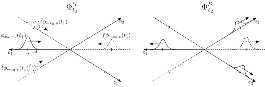
Figure 2: We represent the state $\Phi_{t}^{S}$ for $t=t_{1}$ and $t=t_{2}$. The continuous lines stand for the real graph, the dashed lines represent the extension of each edge to negative values of $x$. At time $t=t_{1}$ only the vector $\Phi^{S,in}$ is significantly supported on the real graph. At time $t=t_{2}$ only the state $\Phi^{S,out}$ has relevant support on the real graph, while the body of the soliton in $\Phi^{S,in}$ has moved to the negative axis associated with the first edge.

Proposition 5.4.

Let $t\in\left(t_{1},t_{2}\right)$ then there exists $v_{0}>0$ such that for all $v>v_{0}$

$$\|\Psi_{t}-\Phi^{S}_{t}\|\leqslant C_{1}v^{-\frac{\delta}{2}}\,,$$ (5.22)

moreover

$$\|\Psi_{t_{2}}-\Phi^{S,out}_{t_{2}}\|\leqslant C_{2}v^{-\frac{\delta}{2}}\,,$$ (5.23)

where $C_{1}$ and $C_{2}$ are positive constants which do not depend on $t$ and $v$.

Proof.

From the definition of $\Psi_{t}$, see equation (4.4), we have

$$\Psi_{t}=\ e^{-iH(t-t_{1})}\Psi_{t_{1}}+i\int_{t_{1}}^{t}ds\,e^{-iH(t-s)}|\Psi_{s}|^{2}\Psi_{s}\,.$$

We start with the trivial estimate

$$\big{\|}\Psi_{t}-\Phi^{S}_{t}\big{\|}$$ (5.24)

$$\leqslant\big{\|}\Psi_{t}-e^{-iH(t-t_{1})}\Psi_{t_{1}}\big{\|}+\big{\|}e^{-iH(t-t_{1})}\Psi_{t_{1}}-e^{-iH(t-t_{1})}\Phi_{t_{1}}^{S,in}\big{\|}+\big{\|}e^{-iH(t-t_{1})}\Phi_{t_{1}}^{S,in}-\Phi^{S}_{t}\big{\|}$$

and estimate the r.h.s. term by term. The estimates involved in the analysis of the first term are similar to the ones used in the previous proposition, thus we omit the details. Similarly to what was done above we set $X_{t_{1},t_{2}}=L^{\infty}_{[t_{1},t_{2}]}L^{2}\cap L^{6}_{[t_{1},t_{2}]}L^{6}$, then by Strichartz estimates (see equation (5.12) and proposition 2.3)

$$\big{\|}\Psi-e^{-iH(\cdot-t_{1})}\Psi_{t_{1}}\big{\|}_{X_{t_{1},t_{2}}}\leqslant\bigg{\|}\int_{t_{1}}^{\cdot}ds\,e^{-iH(\cdot-s)}|\Psi_{s}|^{2}\Psi_{s}\bigg{\|}_{X_{t_{1},t_{2}}}\leqslant C(t_{2}-t_{1})^{1/2}\big{\|}\Psi\big{\|}_{X_{t_{1},t_{2}}}^{3}\,,$$ (5.25)

$$\big{\|}e^{-iH(\cdot-t_{1})}\Psi_{t_{1}}\big{\|}_{X_{t_{1},t_{2}}}\leqslant C\big{\|}\Psi_{t_{1}}\big{\|}\,,$$

which imply

$$\big{\|}\Psi\big{\|}_{X_{t_{1},t_{2}}}\leqslant C\big{\|}\Psi_{t_{1}}\big{\|}+C(t_{2}-t_{1})^{1/2}\big{\|}\Psi\big{\|}_{X_{t_{1},t_{2}}}^{3}\,.$$

By lemma 5.2 one has that if $(t_{2}-t_{1})\leqslant\big{[}8C^{3}\|\Psi_{t_{1}}\|^{2}+4C^{2}\|\Psi_{t_{1}}\|\big{]}^{-2}$, then $\|\Psi\|_{X_{t_{1},t_{2}}}\leqslant 2C\|\Psi_{t_{1}}\|$; using this estimate in the inequality (5.25) we get

$$\big{\|}\Psi_{t}-e^{-iH(t-t_{1})}\Psi_{t_{1}}\big{\|}\leqslant\big{\|}\Psi-e^{-iH(\cdot-t_{1})}\Psi_{t_{1}}\big{\|}_{X_{t_{1},t_{2}}}\leqslant C(t_{2}-t_{1})^{1/2}\big{\|}\Psi_{t_{1}}\big{\|}^{3}\leqslant Cv^{-\delta/2}$$ (5.26)

where we used $t_{2}-t_{1}=2v^{-\delta}$.

We proceed now with the estimate of the second term on the r.h.s. of inequality (5.24). Let us set

$$\Phi_{t_{1}}^{tail}:=\begin{pmatrix}0\\ \\ \phi_{-x_{0},v}(t_{1})\\ \\ 0\end{pmatrix}\;.$$

We notice that $\Phi_{t_{1}}^{S,in}+\Phi_{t_{1}}^{tail}=\Phi_{t_{1}}$ where the vector $\Phi_{t}$ was defined in equation (5.1) and rewrite $\Psi_{t_{1}}$ by adding and subtracting $\Phi_{t_{1}}$

$$\Psi_{t_{1}}=\Psi_{t_{1}}-\Phi_{t_{1}}+\Phi_{t_{1}}^{S,in}+\Phi_{t_{1}}^{tail}\,.$$

The following trivial inequality holds true

$$\big{\|}e^{-iH(t-t_{1})}\Psi_{t_{1}}-e^{-iH(t-t_{1})}\Phi_{t_{1}}^{S,in}\big{\|}\leqslant\big{\|}\Psi_{t_{1}}-\Phi_{t_{1}}\big{\|}+\big{\|}\Phi_{t_{1}}^{tail}\big{\|}\leqslant Ce^{-v^{1-\delta}}$$ (5.27)

where in the latter estimate we used proposition 5.3 and the fact that $\|\Phi_{t_{1}}^{tail}\|\leqslant 2e^{-v^{1-\delta}}$.

Let us consider now the last term on the r.h.s. of inequality (5.24). We are going to prove that for all $t\in(t_{1},t_{2})$ and for $v$ big enough

$$\big{\|}e^{-iH(t-t_{1})}\Phi_{t_{1}}^{S,in}-\Phi^{S}_{t}\big{\|}\leqslant Cv^{-\delta}\,.$$ (5.28)

Let us introduce the functions

$$\phi^{-}_{t}(x):=\int_{0}^{\infty}U_{t-t_{1}}(x-y)\phi_{x_{0},-v}(y,t_{1})dy$$ (5.29)

and

$$\phi^{+}_{t}(x):=\int_{0}^{\infty}U_{t-t_{1}}(x+y)\phi_{x_{0},-v}(y,t_{1})dy\,.$$ (5.30)

First we prove a preliminary formula for the vector $e^{-iH(t-t_{1})}\Phi^{S,in}_{t_{1}}$ (see equations (5.35) and (5.36) below). For any constant $a>0$, not dependent on $v$ let us consider the term

$$va\int_{0}^{\infty}e^{-uva}\big{[}U^{+}_{t-t_{1}}\phi_{x_{0},-v}(t_{1})\big{]}(u+x)du$$

$$= va\int_{0}^{\infty}du\int_{0}^{\infty}dy\,e^{-uva}U_{t-t_{1}}(u+x+y)e^{i\varphi(t_{1})}e^{-i\frac{v}{2}y}\phi(y-x_{0}+vt_{1})$$

where we set $\varphi(t):=-t\frac{v^{2}}{4}+t$. By integrating by parts we obtain the equality

$$va\int_{0}^{\infty}e^{-uva}\big{[}U^{+}_{t-t_{1}}\phi_{x_{0},-v}(t_{1})\big{]}(u+x)du$$ (5.31)

$$= 2ia\int_{0}^{\infty}du\int_{0}^{\infty}dy\,e^{-uva}U_{t-t_{1}}(u+x+y)e^{i\varphi(t_{1})}\bigg{[}\frac{d}{dy}e^{-i\frac{v}{2}y}\bigg{]}\phi(y-x_{0}+vt_{1})$$

$$= A_{1}(x,t)+A_{2}(x,t)+A_{3}(x,t)$$

with

$$A_{1}(x,t):=-2ia\int_{0}^{\infty}du\,e^{-uva}U_{t-t_{1}}(u+x)e^{i\varphi(t_{1})}\phi(-x_{0}+vt_{1})$$

$$A_{2}(x,t):=-2ia\int_{0}^{\infty}du\int_{0}^{\infty}dy\,e^{-uva}\bigg{[}\frac{d}{dy}U_{t-t_{1}}(u+x+y)\bigg{]}e^{i\varphi(t_{1})}e^{-i\frac{v}{2}y}\phi(y-x_{0}+vt_{1})\\$$

$$A_{3}(x,t):=-2ia\int_{0}^{\infty}du\int_{0}^{\infty}dy\,e^{-uva}U_{t-t_{1}}(u+x+y)e^{i\varphi(t_{1})}e^{-i\frac{v}{2}y}\bigg{[}\frac{d}{dy}\phi(y-x_{0}+vt_{1})\bigg{]}\,.$$

We notice that

$$\bigg{\|}\int_{0}^{\infty}du\,e^{-uva}U_{t-t_{1}}(u+\cdot)\bigg{\|}_{L^{2}(\mathbb{R}^{+})}\leqslant\bigg{\|}\int_{0}^{\infty}du\,e^{-uva}U_{t-t_{1}}(u+\cdot)\bigg{\|}_{L^{2}(\mathbb{R})}=\|\chi_{+}e^{-va\cdot}\|_{L^{2}(\mathbb{R})}=\sqrt{\frac{1}{2va}}.$$

Then the following estimate for the term $A_{1}$ holds true

$$\|A_{1}(t)\|_{L^{2}(\mathbb{R}^{+})}\leqslant 2a\bigg{\|}\int_{0}^{\infty}du\,e^{-uva}U_{t-t_{1}}(u+\cdot)\bigg{\|}_{L^{2}(\mathbb{R}^{+})}|\phi(-x_{0}+vt_{1})|\leqslant C\,\frac{e^{-v^{1-\delta}}}{v^{1/2}}\,.$$ (5.32)

The term $A_{3}$ is estimated by

$$\|A_{3}(t)\|_{L^{2}(\mathbb{R}^{+})}\leqslant 2a\int_{0}^{\infty}du\,e^{-uva}\big{\|}\big{[}U_{t-t_{1}}\chi_{+}e^{-i\frac{v}{2}\cdot}\phi^{\prime}(\cdot-x_{0}+vt_{1})\big{]}\big{(}-(u+\cdot)\big{)}\big{\|}_{L^{2}(\mathbb{R}^{+})}$$ (5.33)

$$\leqslant 2\big{\|}\phi^{\prime}\big{\|}_{L^{2}(\mathbb{R})}a\int_{0}^{\infty}du\,e^{-uva}\leqslant\frac{C}{v}\,,$$

where we used the equality $[U_{t}^{+}f](x)=[U_{t}\chi_{+}f](-x)$.

We compute finally the term $A_{2}$. By integration by parts

$$A_{2}(x,t)= -2ia\int_{0}^{\infty}du\int_{0}^{\infty}dy\,e^{-uva}\bigg{[}\frac{d}{du}U_{t-t_{1}}(u+x+y)\bigg{]}e^{i\varphi(t_{1})}e^{-i\frac{v}{2}y}\phi(y-x_{0}+vt_{1})$$

$$= 2ia\phi^{+}_{t}(x)-2iva^{2}\int_{0}^{\infty}e^{-uva}\big{[}U^{+}_{t-t_{1}}\phi_{x_{0},-v}(t_{1})\big{]}(u+x)du\,,$$

where the function $\phi^{+}_{t}$ was defined in equation (5.30). Using the last equality in the equation (LABEL:misunderstood) we get

$$va\int_{0}^{\infty}e^{-uva}\big{[}U^{+}_{t-t_{1}}\phi_{x_{0},-v}(t_{1})\big{]}(u+x)du=\frac{2ia}{1+2ia}\phi^{+}_{t}(x)+\frac{A_{1}(x,t)+A_{3}(x,t)}{1+2ia}\,.$$ (5.34)

From the definition of $\Phi^{S,in}_{t}$ and using the last equality with $a=\tilde{\alpha}/3$ in the formula for the integral kernel of $e^{-iH_{\delta}^{\tilde{\alpha}v}t}$, see equation (2.21), it follows that

$$e^{-iH_{\delta}^{\tilde{\alpha}v}(t-t_{1})}\Phi_{t_{1}}^{S,in}=e^{-iH_{\delta}^{\tilde{\alpha}v}(t-t_{1})}\begin{pmatrix}\phi_{x_{0},-v}(t_{1})\\ \\ 0\\ \\ 0\end{pmatrix}=\begin{pmatrix}\phi^{-}_{t}-\frac{1+2i\tilde{\alpha}}{3+2i\tilde{\alpha}}\phi^{+}_{t}\\ \\ \frac{2}{3+2i\tilde{\alpha}}\phi^{+}_{t}\\ \\ \frac{2}{3+2i\tilde{\alpha}}\phi^{+}_{t}\end{pmatrix}-\frac{2}{3}\begin{pmatrix}A_{\tilde{\alpha}}(t)\\ \\ A_{\tilde{\alpha}}(t)\\ \\ A_{\tilde{\alpha}}(t)\end{pmatrix}\,,$$ (5.35)

where the function $\phi_{t}^{-}$ was defined in equation (5.29) and we set $A_{\tilde{\alpha}}(x,t):=\big{[}(A_{1}(x,t)+A_{3}(x,t))/(1+2ia)\big{]}\big{|}_{a=\tilde{\alpha}/3}$. Similarly using equality (5.34) with $a=3/\tilde{\beta}$ in the formula for the integral kernel of the propagator $e^{-iH_{\delta^{\prime}}^{\tilde{\beta}/v}t}$, see equation (2.22), we get

$$e^{-iH_{\delta^{\prime}}^{\tilde{\beta}/v}(t-t_{1})}\Phi_{t_{1}}^{S,in}=\begin{pmatrix}\phi^{-}_{t}+\frac{\tilde{\beta}+2i}{\tilde{\beta}+6i}\phi^{+}_{t}\\ \\ -\frac{4i}{\tilde{\beta}+6i}\phi^{+}_{t}\\ \\ -\frac{4i}{\tilde{\beta}+6i}\phi^{+}_{t}\end{pmatrix}-\frac{2}{3}\begin{pmatrix}A_{\tilde{\beta}}(t)\\ \\ A_{\tilde{\beta}}(t)\\ \\ A_{\tilde{\beta}}(t)\end{pmatrix}$$ (5.36)

where we introduced the notation $A_{\tilde{\beta}}(x,t):=\big{[}(A_{1}(x,t)+A_{3}(x,t))/(1+2ia)\big{]}\big{|}_{a=3/\tilde{\beta}}$. We notice that the analogous formula for $e^{-iH_{F}(t-t_{1})}\Phi_{t_{1}}^{S,in}$ can be obtained from equation (5.35) by setting $\tilde{\alpha}=0$ and $A_{\tilde{\alpha}}=0$.

To get the estimate (5.28) we show that, at the cost of an error of the order $(t_{2}-t_{1})$, for $t\in(t_{1},t_{2})$, the functions $\phi^{-}_{t}(x)$ and $\phi^{+}_{t}(x)$ can be approximated by the solitons $\phi_{x_{0},-v}(x,t)$ and $\phi_{-x_{0},v}(x,t)$ respectively. We consider first the function $\phi^{+}_{t}$, by adding and subtracting a suitable term to the r.h.s. of equation (5.30) we get

$$\phi^{+}_{t}(x)= \int_{-\infty}^{\infty}U_{t-t_{1}}(x+y)\phi_{x_{0},-v}(y,t_{1})+i\int_{t_{1}}^{t}ds\int_{-\infty}^{\infty}U_{t-s}(x+y)|\phi_{x_{0},-v}(y,s)|^{2}\phi_{x_{0},-v}(y,s)dy$$ (5.37)

$$-\int_{-\infty}^{0}U_{t-t_{1}}(x+y)\phi_{x_{0},-v}(y,t_{1})dy-i\int_{t_{1}}^{t}ds\int_{-\infty}^{\infty}U_{t-s}(x+y)|\phi_{x_{0},-v}(y,s)|^{2}\phi_{x_{0},-v}(y,s)\,dy$$

$$= \phi_{-x_{0},v}(x,t)+I(x,t)+II(x,t)\,,$$

where we used the fact that $\phi_{x_{0},-v}(-x,t)=\phi_{-x_{0},v}(x,t)$ and we set

$$I(x,t):=-\int_{-\infty}^{0}U_{t-t_{1}}(x+y)\phi_{x_{0},-v}(y,t_{1})dy$$

and

$$II(x,t):=-i\int_{t_{1}}^{t}ds\int_{-\infty}^{\infty}U_{t-s}(x+y)|\phi_{x_{0},-v}(y,s)|^{2}\phi_{x_{0},-v}(y,s)\,dy\,.$$

For the term $I$ we use the estimate

$$\|I\|_{L^{2}(\mathbb{R}^{+})}\leqslant\|\phi(\cdot-x_{0}+vt_{1})\|_{L^{2}(\mathbb{R}^{-})}\leqslant 2e^{-v^{1-\delta}}\,.$$

The term $II$ is estimated by

$$\|II\|_{L^{2}(\mathbb{R}^{+})}\leqslant(t-t_{1})\|\phi^{3}\|_{L^{2}(\mathbb{R})}\leqslant Cv^{-\delta}\,.$$

Similarly, for the function $\phi^{-}_{t_{2}}$, we get

$$\phi^{-}_{t}(x)=\phi_{x_{0},-v}(x,t)+III(x,t)+IV(x,t)$$ (5.38)

where we set

$$III(x,t):=-\int_{-\infty}^{0}U_{t-t_{1}}(x-y)\phi_{x_{0},-v}(t_{1},y)dy$$

and

$$IV(x,t):=-i\int_{t_{1}}^{t}ds\int_{-\infty}^{\infty}U_{t-s}(x-y)|\phi_{x_{0},-v}(s,y)|^{2}\phi_{x_{0},-v}(s,y)\,dy\,.$$

For $t\in(t_{1},t_{2})$ the estimates

$$\|III\|_{L^{2}(\mathbb{R}^{+})}\leqslant 2e^{-v^{1-\delta}}\;;\quad\|IV\|_{L^{2}(\mathbb{R}^{+})}\leqslant Cv^{-\delta}$$

are similar to the ones given above for the terms $I$ and $II$. Then from equations (5.37) and (5.38) we have

$$\|\phi^{+}_{t}-\phi_{-x_{0},v}(t)\|_{L^{2}(\mathbb{R}^{+})}\leqslant C[e^{-v^{1-\delta}}+v^{-\delta}]\,,\quad\|\phi^{-}_{t}-\phi_{x_{0},-v}(t)\|_{L^{2}(\mathbb{R}^{+})}\leqslant C[e^{-v^{1-\delta}}+v^{-\delta}]$$

for all $t\in(t_{1},t_{2})$. By using the last estimates and the estimates (5.32) and (5.33) in equations (5.35) and (5.36) we get

$$\big{\|}e^{-iH(t-t_{1})}\Phi_{t_{1}}^{S,in}-\Phi^{S}_{t}\big{\|}\leqslant C\bigg{[}e^{-v^{1-\delta}}+v^{-\delta}+\frac{e^{-v^{1-\delta}}}{v^{1/2}}+\frac{1}{v}\bigg{]}$$

which in turn implies that for $v$ big enough the estimate (5.28) holds true.

Using estimates (5.26), (5.27) and (5.28) in the inequality (5.24) we get the estimate (5.22).

The estimate (5.23) is a consequence of estimate (5.22) and of the fact that $\|\Phi^{S}_{t_{2}}-\Phi^{S,out}_{t_{2}}\|=\|\Phi^{S,in}_{t_{2}}\|\leqslant Ce^{-v^{1-\delta}}$. ∎

Remark 5.5.

Notice that estimate (5.22), although not strictly necessary for the proof of theorem 4.3, enforces the picture that in the phase 2 a scattering event is occurring. The true wavefunction can be approximated by the superposition of an incoming and an outgoing wavefunction. At the end of this phase, only the outgoing wavefunction is not negligibile.

5.3 Phase 3

Let us put $t_{3}=t_{2}+T\ln v$. We call “phase 3” the evolution of the system in the time interval $(t_{2},t_{3})$. The approximation of $\Psi_{t}$ during this time interval is the content of theorem 4.3.

We recall the following result (see [17]).

Proposition 5.6.

Let $\phi^{tr}_{t}$ and $\phi^{ref}_{t}$ be defined as it was done in equations (4.12) and (4.13) above. Then $\forall k\in\mathbb{N}$ there exist two constants $c(k)>0$ and $\sigma(k)>0$ such that

$$\|\phi^{\gamma}_{t}\|_{L^{2}(\mathbb{R}^{-})}+\|\phi^{\gamma}_{t}\|_{L^{\infty}(\mathbb{R}^{-})}\leqslant\frac{c(k)(\ln v)^{\sigma(k)}}{v^{k(1-\delta)}}$$ (5.39)

for $\gamma=\{\text{ref},\text{tr}\}$, uniformly in $t\in[0,T\ln v]$.

Notice that also the norms $\|\phi^{\gamma}_{t}\|_{L^{p}(\mathbb{R}^{-})}$, for $2\leqslant p\leqslant\infty$, are estimated by the r.h.s. of (5.39). Now we can prove theorem 4.3

Proof of Theorem 4.3..

The strategy of the proof closely follows proposition 5.3. We will just sketch the common part of the proof while proving in details the different estimates.

Let us define $\Xi_{t}:=\Psi_{t}-\sum_{j=1}^{3}\Phi^{j}_{t}$ where the vectors $\Phi^{j}_{t}$ were given in equation (4.9) and fix $t_{a}\in[t_{2},t_{3}]$. From equations (4.4) and (4.9) it follows that the vector $\Xi_{t}$ satisfies the following integral equation

$$\Xi_{t}= e^{-iH(t-t_{a})}\Xi_{t_{a}}$$ (5.40)

$$+\sum_{j=1}^{3}\bigg{[}\Big{(}e^{-iH(t-t_{a})}-e^{-iH_{j}(t-t_{a})}\Big{)}\Phi^{j}_{t_{a}}+i\int_{t_{a}}^{t}ds\,\Big{(}e^{-iH(t-s)}-e^{-iH_{j}(t-s)}\Big{)}|\Phi^{j}_{s}|^{2}\Phi^{j}_{s}\bigg{]}$$

$$+i\int_{t_{a}}^{t}ds\,e^{-iH(t-s)}\sum_{j_{1},j_{2},j_{3}}(1-\delta_{j_{1}j_{2}}\delta_{j_{2}j_{3}})\overline{\Phi^{j_{1}}_{s}}\Phi^{j_{2}}_{s}\Phi^{j_{3}}_{s}$$

$$+i\int_{t_{a}}^{t}ds\,e^{-iH(t-s)}\bigg{[}\bigg{|}\Xi_{s}+\sum_{j=1}^{3}\Phi^{j}_{s}\bigg{|}^{2}\Xi_{s}+|\Xi_{s}|^{2}\sum_{j=1}^{3}\Phi^{j}_{s}+2\operatorname{Re}\,\bigg{[}\overline{\Xi_{s}}\sum_{j=1}^{3}\Phi^{j}_{s}\bigg{]}\sum_{j=1}^{3}\Phi^{j}_{s}\bigg{]}$$

$$= e^{-iH(t-t_{a})}\Xi_{t_{a}}+G(t_{a},t)$$

$$+i\int_{t_{a}}^{t}ds\,e^{-iH(t-s)}\bigg{[}\bigg{|}\Xi_{s}+\sum_{j=1}^{3}\Phi^{j}_{s}\bigg{|}^{2}\Xi_{s}+|\Xi_{s}|^{2}\sum_{j=1}^{3}\Phi^{j}_{s}+2\operatorname{Re}\,\bigg{[}\overline{\Xi_{s}}\sum_{j=1}^{3}\Phi^{j}_{s}\bigg{]}\sum_{j=1}^{3}\Phi^{j}_{s}\bigg{]}\,.$$

Let us fix $t_{b}\in[t_{a},t_{3}]$ and let $X_{t_{a},t_{b}}=L^{\infty}_{[t_{a},t_{b}]}L^{2}\cap L^{6}_{[t_{a},t_{b}]}L^{6}$. Using the Strichartz estimates as it was done in proposition 5.3 (see equations (5.9) - (5.13)), it is straightforward to prove that

$$\|\Xi\|_{X_{t_{a},t_{b}}}\leqslant\widetilde{C}\left[\|\Xi_{t_{a}}\|+\|G(t_{a},\cdot)\|_{X_{t_{a},t_{b}}}+(t_{b}-t_{a})^{1/2}\left(\|\Xi\|_{X_{t_{a},t_{b}}}^{2}+\|\Xi\|_{X_{t_{a},t_{b}}}^{3}\right)\right]$$

where $\widetilde{C}$ depends only on the constants appearing in the Strichartz estimates. Using lemma 5.2 as it was done in the proof of proposition 5.3 it follows that there exists $\tau>0$ such that, for any $t\in[t_{2},t_{3})$ one has $\|\Xi\|_{X_{t,t+\tau}}\leqslant\ 2\widetilde{C}\ \|\Xi_{t}\|+2\widetilde{C}\ \|G(t,\cdot)\|_{X_{t,t+\tau}}$.

We divide the interval $[t_{2},t_{3}]$ in $N+1$ subintervals: $[t_{2}+j\tau,t_{2}+(j+1)\tau)$, with $j=0,...,N-1$; and $[t_{2}+N\tau,t_{3})$, and where $N$ is the integer part of $(t_{3}-t_{2})/\tau$.

Then proceeding by induction as we did in the proof of proposition 5.3, see equations (5.14) and (5.15), we get the inequality

$$\|\Xi\|_{X_{t_{2},t_{3}}}\ \leqslant\sum_{j=0}^{N}(2\widetilde{C})^{j+1}\|\Xi_{t_{2}}\|+\sum_{j=0}^{N}\sum_{k=0}^{j}(2\widetilde{C})^{j+1-k}\|G(t_{2}+k\tau,\cdot)\|_{X_{t_{2}+k\tau,\min\{t_{3},t_{2}+(k+1)\tau\}}}\,.$$ (5.41)

Now we estimate the initial data $\|\Xi_{t_{2}}\|$ and the source term $\|G(t_{a},\cdot)\|_{X_{t_{a},t_{b}}}$ with $t_{2}\leqslant t_{a}\leqslant t_{b}\leqslant t_{3}$ and $t_{b}-t_{a}\leqslant\tau$.

By proposition 5.4 (estimate (5.33)) and using the definitions (4.5) - (4.7) one has

$$\Xi_{t_{2}}=\Psi_{t_{2}}-\sum_{j=1}^{3}\Phi^{j}_{t_{2}}=\Psi_{t_{2}}-\Phi^{S,out}_{t_{2}}-\begin{pmatrix}\tilde{t}\,\phi_{x_{0},-v}(t_{2})\\ \\ \tilde{r}\,\phi_{x_{0},-v}(t_{2})\\ \\ \tilde{t}\,\phi_{x_{0},-v}(t_{2})\end{pmatrix}\,,$$

with $\|\Psi_{t_{2}}-\Phi^{S,out}_{t_{2}}\|\leqslant Cv^{-\delta/2}$. Since

$$\int_{0}^{\infty}|\phi_{x_{0},-v}(x,t_{2})|^{2}dx=\int_{0}^{\infty}|\phi(x-x_{0}+vt_{2})|^{2}dx=2\int_{v^{1-\delta}}^{\infty}{\rm{sech}}(x)^{2}dx=\frac{4e^{-2v^{1-\delta}}}{1+e^{-2v^{1-\delta}}}\leqslant 4e^{-2v^{1-\delta}}$$

we have

$$\|\Xi_{t_{2}}\|\leqslant C\big{(}v^{-\frac{\delta}{2}}+e^{-2v^{1-\delta}}\big{)}\,\leqslant Cv^{-\frac{\delta}{2}}\,.$$ (5.42)

Let us now consider the source term $G(t_{a},t)$. We use the estimate $\|G(t_{a},\cdot)\|_{X_{t_{a},t_{b}}}\leqslant\|G(t_{2},\cdot)\|_{X_{t_{2},t_{3}}}$. To simplify the notation we set $G(t)\equiv G(t_{2},t)$ and

$$G_{1}(t):=\sum_{j=1}^{3}\bigg{[}\Big{(}e^{-iH(t-t_{2})}-e^{-iH_{j}(t-t_{2})}\Big{)}\Phi^{j}_{t_{2}}+i\int_{t_{2}}^{t}ds\,\Big{(}e^{-iH(t-s)}-e^{-iH_{j}(t-s)}\Big{)}|\Phi^{j}_{s}|^{2}\Phi^{j}_{s}\bigg{]}$$

$$G_{2}(t):=i\int_{t_{2}}^{t}ds\,e^{-iH(t-s)}\sum_{j_{1},j_{2},j_{3}}(1-\delta_{j_{1}j_{2}}\delta_{j_{2}j_{3}})\overline{\Phi^{j_{1}}_{s}}\Phi^{j_{2}}_{s}\Phi^{j_{3}}_{s}\,.$$

By the definition of $G(t_{a},t)$, see equation (5.40) it follows that

$$G(t)=G_{1}(t)+G_{2}(t)\,;$$

we estimate $G_{1}(t)$ and $G_{2}(t)$ separately.

We proceed first with the estimate of the term $G_{1}$. From equations (2.20), (2.21), (2.22) and (2.31) one can see that for any (column) vector $F=(F_{1},F_{2},F_{3})\in L^{2}$

$$\big{[}e^{-iHt}-e^{-iH_{j}t}\big{]}F=\mathbb{M}_{j}\begin{pmatrix}U^{+}_{t}F_{1}\\ \\ U^{+}_{t}F_{2}\\ \\ U^{+}_{t}F_{3}\end{pmatrix}-\frac{2}{3}\mathbb{J}\begin{pmatrix}va\int_{0}^{\infty}e^{-uva}\big{[}U^{+}_{t}F_{1}\big{]}(u+\cdot)du\\ \\ va\int_{0}^{\infty}e^{-uva}\big{[}U^{+}_{t}F_{2}\big{]}(u+\cdot)du\\ \\ va\int_{0}^{\infty}e^{-uva}\big{[}U^{+}_{t}F_{3}\big{]}(u+\cdot)du\end{pmatrix}\qquad j=1,2,3\,,$$

where the constant $a$ and the matrices $\mathbb{M}_{j}$ must be chosen accordingly to the Hamiltonian $H$:
for $H=H_{\delta}^{\tilde{\alpha}v}$,

$$a=\frac{\tilde{\alpha}}{3}\;,\qquad\mathbb{M}_{j}=-\mathbb{I}+\frac{2}{3}\mathbb{J}-\mathbb{T}_{j}\,;$$

for $H=H_{\delta^{\prime}}^{\tilde{\beta}/v}$,

$$a=\frac{3}{\tilde{\beta}}\;,\qquad\mathbb{M}_{j}=\mathbb{I}-\mathbb{T}_{j}\,;$$

and the formula for $H=H_{F}$ can be obtained by setting $\tilde{\alpha}=0$ in the formula for $H=H_{\delta}^{\alpha}$.

Then, denoting by $\big{(}G_{1}(x,t)\big{)}_{l}$, $l=1,2,3$, the $l$-th component of the vector $G_{1}$ one has

$$\big{(}G_{1}(x,t)\big{)}_{l}=\big{(}\widetilde{G}_{1}(x,t)\big{)}_{l}+\big{(}\widehat{G}_{1}(x,t)\big{)}_{l}\,,$$

with

$$\big{(}\widetilde{G}_{1}(x,t)\big{)}_{l}:=\sum_{j,k=1}^{3}\big{(}\mathbb{M}_{j}\big{)}_{lk}\bigg{[}\big{[}U^{+}_{t-t_{2}}\big{(}\Phi^{j}_{t_{2}}\big{)}_{k}\big{]}(x)+i\int_{t_{2}}^{t}ds\big{[}U^{+}_{t-s}\big{|}\big{(}\Phi^{j}_{s}\big{)}_{k}\big{|}^{2}\big{(}\Phi^{j}_{s}\big{)}_{k}\big{]}(x)\bigg{]}$$

$$\big{(}\widehat{G}_{1}(x,t)\big{)}_{l}:=-\frac{2va}{3}\sum_{j,k=1}^{3}\int_{0}^{\infty}e^{-vua}\bigg{[}\big{[}U^{+}_{t-t_{2}}\big{(}\Phi^{j}_{t_{2}}\big{)}_{k}\big{]}(u+x)+i\int_{t_{2}}^{t}ds\big{[}U^{+}_{t-s}\big{|}\big{(}\Phi^{j}_{s}\big{)}_{k}\big{|}^{2}\big{(}\Phi^{j}_{s}\big{)}_{k}\big{]}(u+x)\bigg{]}du\,.$$

From the definition of the vectors $\Phi^{j}_{t}$, see equations (4.10) - (4.11), we see that for each $l=1,2,3$ the function $\big{(}\widetilde{G}_{1}(x,t)\big{)}_{l}$ is a linear combination of four functions, $f^{\gamma,+}_{t}$ and $f^{\gamma,-}_{t}$, with $\gamma$ being equal to $ref$ and $tr$, given by

$$f^{\gamma,+}_{t}(x):=e^{-i\frac{v^{2}}{4}t_{2}}e^{it_{2}}\bigg{[}\int_{0}^{\infty}U_{t-t_{2}}(x+y)\phi_{0}^{\gamma}(y)dy+i\int_{t_{2}}^{t}ds\int_{0}^{\infty}U_{t-s}(x+y)|\phi^{\gamma}_{s-t_{2}}(y)|^{2}\phi^{\gamma}_{s-t_{2}}(y)dy\bigg{]}$$ (5.43)

and

$$f^{\gamma,-}_{t}(x):=e^{-i\frac{v^{2}}{4}t_{2}}e^{it_{2}}\bigg{[}\int_{0}^{\infty}U_{t-t_{2}}(x+y)\phi_{0}^{\gamma}(-y)dy+i\int_{t_{2}}^{t}ds\int_{0}^{\infty}U_{t-s}(x+y)|\phi^{\gamma}_{s-t_{2}}(-y)|^{2}\phi^{\gamma}_{s-t_{2}}(-y)dy\bigg{]}\,,$$

where the functions $\phi^{ref}_{t}$ and $\phi^{ref}_{t}$ were defined in equations (4.12) and (4.13) respectively.

Similarly one can see that for each $l=1,2,3$ the function $\big{(}\widehat{G}_{1}(x,t)\big{)}_{l}$ is a linear combination of

$$va\int_{0}^{\infty}e^{-vua}f^{ref,+}_{t}(u+x)du\;,\quad va\int_{0}^{\infty}e^{-vua}f^{tr,+}_{t}(u+x)du\;,$$

$$va\int_{0}^{\infty}e^{-vua}f^{ref,-}_{t}(u+x)du\;,\quad va\int_{0}^{\infty}e^{-vua}f^{tr,-}_{t}(u+x)du\;.$$

First we study the function $f^{\gamma,+}_{t}$. We notice that, adding and subtracting a suitable term in equation (5.43) and using the definitions (4.12) and (4.13), $f^{\gamma,+}_{t}(x)$ can be written as

$$f^{\gamma,+}_{t}(x)=I(x,t)+II(x,t)+III(x,t)\,,$$

with

$$I(x,t):=e^{-i\frac{v^{2}}{4}t_{2}}e^{it_{2}}\phi^{\gamma}_{t-t_{2}}(-x)$$

$$II(x,t):=-e^{-i\frac{v^{2}}{4}t_{2}}e^{it_{2}}\int_{0}^{\infty}U_{t-t_{2}}(x-y)\phi_{0}^{\alpha}(-y)dy$$

$$III(x,t):=-ie^{-i\frac{v^{2}}{4}t_{2}}e^{it_{2}}\int_{t_{2}}^{t}ds\int_{0}^{\infty}U_{t-s}(x-y)|\phi^{\gamma}_{s-t_{2}}(-y)|^{2}\phi^{\gamma}_{s-t_{2}}(-y)dy\,.$$

Similarly to what was done above, we set $X_{t_{2},t_{3}}(\mathbb{R}^{\pm})=L^{\infty}_{[t_{2},t_{3}]}L^{2}(\mathbb{R}^{\pm})\cap L^{6}_{[t_{2},t_{3}]}L^{6}(\mathbb{R}^{\pm})$. By proposition 5.6, we have

$$\|I\|_{X_{t_{2},t_{3}}(\mathbb{R}^{+})}=\|\phi^{\gamma}_{\cdot-t_{2}}\|_{X_{t_{2},t_{3}}(\mathbb{R}^{-})}\leqslant\frac{c^{\prime}(k)(\ln v)^{\sigma^{\prime}(k)}}{v^{k(1-\delta)}}$$ (5.44)

where $c^{\prime}(k)$ and $\sigma^{\prime}(k)$ are constants, different from the one appearing in proposition 5.6. For our purposes we do not need to compute them.

Using the one dimensional Strichartz estimates for $U_{t}$, we have

$$\|II\|_{X_{t_{2},t_{3}}(\mathbb{R}^{+})}\leqslant C\|\chi_{-}\phi_{0}^{\gamma}\|_{L^{2}({\mathbb{R}})}\leqslant Ce^{-2v^{1-\delta}}\,.$$ (5.45)

Finally, the term ${III}$ can be estimated using the inhomogeneous Strichartz estimate and proposition 5.6

$$\|III\|_{X_{t_{2},t_{3}}(\mathbb{R}^{+})}\leqslant C\|(\chi_{-}\phi^{\gamma}_{\cdot-t_{2}})^{3}\|_{L^{1}_{[t_{2},t_{3}]}L^{2}({\mathbb{R}})}\leqslant C\bigg{[}\frac{c(k)(\ln v)^{\sigma(k)^{\prime}}}{v^{k(1-\delta)}}\bigg{]}^{3}\,.$$ (5.46)

Collecting the estimates (5.44), (5.45) and (5.46), it follows that

$$\|f^{\gamma,+}_{\cdot}\|_{X_{t_{2},t_{3}}(\mathbb{R}^{+})}\leqslant C\bigg{[}\frac{c(k)(\ln v)^{\sigma(k)^{\prime}}}{v^{k(1-\delta)}}\bigg{]}\,.$$

The estimate of $f^{\gamma,-}_{t}$ is similar and we omit it. We have proved that for some $c^{\prime}(k)$ and $\sigma^{\prime}(k)$ possibly bigger than $c(k)$ and $\sigma(k)$ we have:

$$\|\widetilde{G}_{1}\|_{X_{t_{2},t_{3}}}\leqslant C\bigg{[}\frac{c^{\prime}(k)(\ln v)^{\sigma^{\prime}(k)}}{v^{k(1-\delta)}}\bigg{]}\,,$$

where $\widetilde{G}_{1}$ is the vector in $L^{2}$ with components $\big{(}\widetilde{G}_{1}(x,t)\big{)}_{l}$, $l=1,2,3$.

The estimate of $\widehat{G}_{1}(t)=\big{(}\big{(}\widehat{G}_{1}(t)\big{)}_{1},\big{(}\widehat{G}_{1}(t)\big{)}_{2},\big{(}\widehat{G}_{1}(t)\big{)}_{3}\big{)}$ is a trivial consequence of the fact that

$$\bigg{\|}va\int_{0}^{\infty}e^{-vua}f^{\gamma,\pm}_{\cdot}(u+\,\cdot\,)du\bigg{\|}_{X_{t_{2},t_{3}}(\mathbb{R}^{+})}\leqslant\big{\|}f^{\gamma,\pm}_{\cdot}\big{\|}_{X_{t_{2},t_{3}}(\mathbb{R}^{+})}\leqslant C\bigg{[}\frac{c(k)(\ln v)^{\sigma(k)^{\prime}}}{v^{k(1-\delta)}}\bigg{]}\,,$$

from which it follows that

$$\|\widehat{G}_{1}\|_{X_{t_{2},t_{3}}}\leqslant C\bigg{[}\frac{c^{\prime}(k)(\ln v)^{\sigma^{\prime}(k)}}{v^{k(1-\delta)}}\bigg{]}\,;$$

and

$$\|G_{1}\|_{X_{t_{2},t_{3}}}\leqslant C\bigg{[}\frac{c^{\prime}(k)(\ln v)^{\sigma^{\prime}(k)}}{v^{k(1-\delta)}}\bigg{]}\,.$$ (5.47)

We analyse now the term $G_{2}$. Due to the presence of $(1-\delta_{j_{1}j_{2}}\delta_{j_{2}j_{3}})$ the components of the vector

$$(1-\delta_{j_{1}j_{2}}\delta_{j_{2}j_{3}})\overline{\Phi^{j_{1}}_{s}}\Phi^{j_{2}}_{s}\Phi^{j_{3}}_{s}$$

contains only terms (up to a phase) like

$$\phi^{\gamma_{1}}_{t-t_{2}}(x)\phi^{\gamma_{2}}_{t-t_{2}}(x)\phi^{\gamma_{3}}_{t-t_{2}}(-x)\quad\textrm{or}\quad\phi^{\gamma_{1}}_{t-t_{2}}(x)\phi^{\gamma_{2}}_{t-t_{2}}(-x)\phi^{\gamma_{3}}_{t-t_{2}}(-x)$$

where $\gamma_{1}$, $\gamma_{2}$ and $\gamma_{3}$ can be $ref$ or $tr$. This can easily be seen by using equations (4.10) - (4.11). By Strichartz methods, it is sufficient to estimate the $L^{1}_{[t_{2},t_{3}]}L^{2}({\mathbb{R}}^{+})$ norm of these terms. Then using Hölder’s inequality we have, for istance

$$\|\phi^{\gamma_{1}}_{t-t_{2}}\phi^{\gamma_{2}}_{t-t_{2}}\phi^{\gamma_{3}}_{t-t_{2}}(-\cdot)\|_{L^{2}(\mathbb{R}^{+})}\leqslant\|\phi^{\gamma_{1}}_{t-t_{2}}\|_{L^{4}(\mathbb{R}^{+})}\|\phi^{\gamma_{2}}_{t-t_{2}}\|_{L^{4}(\mathbb{R}^{+})}\|\phi^{\gamma_{3}}_{t-t_{2}}\|_{L^{\infty}(\mathbb{R}^{-})}\leqslant C\frac{c(k)(\ln v)^{\sigma(k)}}{v^{k(1-\delta)}}\,.$$

The second kind of terms can be estimated in the same way and we obtain

$$\|G_{2}\|_{X_{t_{2},t_{3}}}\leqslant C\bigg{[}\frac{c^{\prime}(k)(\ln v)^{\sigma^{\prime}(k)}}{v^{k(1-\delta)}}\bigg{]}\,,$$

which, together with the estimate (5.47), gives

$$\|G\|_{X_{t_{2},t_{3}}}\leqslant C\bigg{[}\frac{c^{\prime}(k)(\ln v)^{\sigma^{\prime}(k)}}{v^{k(1-\delta)}}\bigg{]}\,.$$ (5.48)

Fix $k$ such that $k(1-\delta)>2$ then for $v$ sufficiently large (5.48) implies

$$\|G\|_{X_{t_{2},t_{3}}}\leqslant\frac{1}{v}\,.$$ (5.49)

$$\|\Xi\|_{X_{t_{2},t_{3}}}\ \leqslant Cv^{-\delta/2}\sum_{j=0}^{N}(2\widetilde{C})^{j+1}+v^{-1}\sum_{j=0}^{N}\sum_{k=0}^{j}(2\widetilde{C})^{j+1-k}$$

$$\leqslant 2Cv^{-\delta/2}(2\widetilde{C})^{N+1}+2v^{-1}\sum_{j=0}^{N}(2\widetilde{C})^{j+1}$$

$$\leqslant 2Cv^{-\delta/2}(2\widetilde{C})^{N+1}+2v^{-1}(2\widetilde{C})^{N+1}\leqslant\widehat{C}v^{-\delta/2}(2\widetilde{C})^{N}\,.$$

Since $N$ is the integer part of $(t_{3}-t_{2})/\tau=\frac{T}{\tau}\ln v$ we have

$$\|\Xi\|_{X_{t_{2},t_{3}}}\ \leqslant\ \widehat{C}v^{-\delta/2+\frac{T}{\tau}\ln(2\widetilde{C})}$$

We can finally set $\tau_{*}\equiv\tau/\ln(2\widetilde{C})$ and $T_{*}=\delta\tau_{*}/2$ and obtain

$${\Vert \mathrm{\Xi }\Vert }_{L_{[t_2,t_3]}^{\mathrm{\infty }}{L}^2}⩽{\Vert \mathrm{\Xi }\Vert }_{X_{t_2,t_3}}⩽\widehat{C}{v}^{-\frac{T_{\ast }-T}{{\tau }_{\ast }}},$$

References

- [1] W. K. Abu Salem, J. Fröhlich, and I. M. Sigal, Colliding solitons for the nonlinear Schrödinger equation, Comm. Math. Phys. 291 (2009), 151–176.
- [2] R. Adami, C. Cacciapuoti, D. Finco and D. Noja, Stationary states of NLS on star graphs, arXiv:1104.3839 [math-ph] (2011), 4pp.
- [3] R. Adami and D. Noja, Existence of dynamics for a 1D NLS equation perturbed with a generalized point defect, J. Phys. A: Math. Theor. 42 (2009), no. 49, 495302, 19pp.
- [4] S. Albeverio, C. Cacciapuoti, and D. Finco, Coupling in the singular limit of thin quantum waveguides, J. Math. Phys. 48 (2007), 032103.
- [5] S. Albeverio, F. Gesztesy, R. Høegh-Krohn, and H. Holden, Solvable models in quantum mechanics: Second edition, AMS Chelsea Publ., 2005, with an Appendix by P. Exner.
- [6] B. Bellazzini, M. Mintchev, Quantum Fields on Star Graphs, J. Phys. A Math. Gen., vol. 39, 1101–1117, 2006.
- [7] G. Berkolaiko, R. Carlson, S. Fulling, and P. Kuchment, Quantum graphs and their applications, Contemporary Math., vol. 415, American Math. Society, Providence, RI, 2006.
- [8] J. Blank, P. Exner, and M. Havlicek, Hilbert spaces operators in quantum physics, Springer, New York, 2008.
- [9] R. Burioni, D. Cassi, P. Sodano, A. Trombettoni, and A. Vezzani, Soliton propagation on chains with simple nonlocal defects, Physica D 216 (2006), 71–76.
- [10] C. Cacciapuoti and P. Exner, Nontrivial edge coupling from a Dirichlet network squeezing: the case of a bent waveguide, J. Phys. A: Math. Theor. 40 (2007), no. 26, F511–F523.
- [11] D. Cao Xiang and A. B. Malomed, Soliton defect collisions in the nonlinear Schrödinger equation, Phys. Lett. A 206 (1995), 177–182.
- [12] S. Cardanobile and D. Mugnolo, Analysis of FitzHugh-Nagumo-Rall model of a neuronal network, Math. Meth. Appl. Sci. 30 (2007), 2281–2308.
- [13] T. Cazenave, Semilinear Schrödinger equations, Courant Lecture Notes in Mathematics, AMS, vol 10, Providence, 2003.
- [14] K. Datchev and J. Holmer, Fast soliton scattering by attractive delta impurities, Comm. Part. Diff. Eq. 34 (2009), 1074–1113.
- [15] P. Exner, Contact interactions on graph superlattices, J. Phys. A: Math. Gen. 29 (1996), no. 1, 87–102.
- [16] R. H. Goodman, P. J. Holmes, and M. I. Weinstein, Strong NLS soliton-defect interactions, Physica D 192 (2004), 215–249.
- [17] J. Holmer, J. Marzuola, and M. Zworski, Fast soliton scattering by delta impurities, Commun. Math. Phys. 274 (2007), 187–216.
- [18] J. Holmer, J. Marzuola, and M. Zworski, Soliton splitting by delta impurities, J. Nonlinear Sci. 7 (2007), 349–367.
- [19] M. Keel and T. Tao, Endpoint Strichartz estimates, Amer. J. Math. 120 (1998), 955–980.
- [20] P. G. Kevrekidis, D. J. Frantzeskakis, G. Theocharis, and I. G. Kevrekidis, Guidance of matter waves through Y-junctions, Phys. Lett. A 317 (2003), 513–522.
- [21] V. Kostrykin and R. Schrader, Kirchhoff’s rule for quantum wires, J. Phys. A: Math. Gen. 32 (1999), no. 4, 595–630.
- [22] P. Kuchment, Quantum graphs. I. Some basic structures, Waves Random Media 14 (2004), no. 1, S107–S128.
- [23] P. Kuchment, Quantum graphs. II. Some spectral properties of quantum and combinatorial graphs, J. Phys. A: Math. Gen. 38 (2005), no. 22, 4887–4900.
- [24] G. Perelman, A remark on soliton-potential interaction for nonlinear Schrödinger equations, Math. Res. Lett. 16 (2009), no. 3, 477–486.
- [25] G. Perelman, Two soliton collision for nonlinear Schrödinger equation in dimension 1, Ann.I.H.Poincaré, AN, in print (2011)
- [26] Z. Sobirov, D. Matrasulov, K. Sabirov, S. Sawada, K. Nakamura, Integrable nonlinear Schrödinger equation on simple networks: Connection formula at vertices Phys. Rev. E 81, 066602 (2010)