Non-equilibrium Relations for Spin Glasses with Gauge Symmetry

Abstract

We study the applications of non-equilibrium relations such as the Jarzynski equality and fluctuation theorem to spin glasses with gauge symmetry. It is shown that the exponentiated free-energy difference appearing in the Jarzynski equality reduces to a simple analytic function written explicitly in terms of the initial and final temperatures if the temperature satisfies a certain condition related to gauge symmetry. This result is used to derive a lower bound on the work done during the non-equilibrium process of temperature change. We also prove identities relating equilibrium and non-equilibrium quantities. These identities suggest a method to evaluate equilibrium quantities from non-equilibrium computations, which may be useful to avoid the problem of slow relaxation in spin glasses.

1 Introduction

Equilibrium and non-equilibrium properties of spin glasses have been studied for many years by experimental, numerical and analytical methods [1, 2, 3]. Although most of the theoretical problems have been solved fairly satisfactorily at the mean-field level [4], it is still difficult to establish analytical results for finite-dimensional systems. Numerical approaches are powerful tools in finite dimensions but are often hampered by slow relaxation if one wishes to evaluate equilibrium quantities at low temperatures, and ingenious methods have been proposed to circumvent this difficulty [5, 6, 7, 8, 9, 10]. In particular, Neal [7] proposed annealed importance sampling, in which one changes the temperature and measures physical quantities in a spirit similar to the Jarzynski equality [11, 12]. Hukushima and Iba [8, 9] improved Neal’s method by incorporating a branching process for the stability of the algorithm. Their method, which they called population annealing, showed outstanding performance comparable to the exchange Monte Carlo.

Non-equilibrium relations such as the Jarzynski equality and fluctuation theorem [13, 14, 15] represent important developments in non-equilibrium statistical physics because they directly relate non-equilibrium and equilibrium quantities (Jarzynski equality) or the probability of a non-equilibrium process and its inverse process (fluctuation theorem). It is the purpose of the present paper to apply the non-equilibrium relations to the context of spin glasses and show that non-trivial simplifications are observed under certain conditions on the system parameters. Several additional non-equilibrium relations are also derived that connect equilibrium and non-equilibrium quantities. These results are not only interesting in their own right but may be useful to extract information from non-equilibrium numerical simulations following the idea of Neal and Hukushima and Iba.

This paper is organized as follows. In the next section, we recall the basic formulation in order to fix the notation and set the stage for further developments in the following sections. In §3, we establish several non-equilibrium relations by using gauge symmetry. In the last section, we give a summary of the results obtained in the present study.

2 Formulation

Let us consider the $\pm J$ Ising model of spin glasses on an arbitrary lattice,

$$H=-\sum_{\langle ij\rangle}J_{ij}S_{i}S_{j},$$ (1)

where the distribution function of quenched randomness is specified as

$$P(\tau_{ij})=p\delta(\tau_{ij}-1)+(1-p)\delta(\tau_{ij}+1)=\frac{\mathrm{e}^{K_{p}\tau_{ij}}}{2\cosh K_{p}}$$ (2)

with $\tau_{ij}$ being the sign of $J_{ij}$ ($J_{ij}=\tau_{ij}J$). The parameter $K_{p}$ has been defined as $\mathrm{e}^{-2K_{p}}=(1-p)/p$. The product $\beta J$ will be written as $K$. The following analyses can readily be applied to other distribution functions of $J_{ij}$ as long as they satisfy a certain type of gauge symmetry [17, 16].

Suppose that the system evolves following a stochastic dynamics governed by the master equation. For simplicity, we will formulate our theory for discrete time steps although the continuous case can be treated similarly. We change the value of the coupling $K$ from $K_{0}$ at $t=t_{0}$ to $K_{T}$ at $t=t_{n}$ in $n$ steps of time evolution, ($K_{0},K_{1},\cdots,K_{n}=K_{T}$). Correspondingly, the spin configuration changes as $\mathbf{S}_{0}$ (at $t=t_{0}$), $\mathbf{S}_{1}$ (at $t=t_{1}$), $\cdots,\mathbf{S}_{n}$ (at $t=t_{n}$). These configurations will be collectively denoted as $\{\mathbf{S}\}$. Notice that each $\mathbf{S}_{i}$ stands for a configuration of $N$ spins at time $t=t_{i}$. The system is assumed to be in equilibrium at $t=t_{0}$.

The fluctuation theorem [13, 14, 15] relates the probability $P_{K_{0}\rightarrow K_{T}}(\{\mathbf{S}\})$ that such a sequence is realized with the probability $P_{K_{T}\rightarrow K_{0}}(\{\mathbf{S}\})$ of the inverse process as

$$\frac{P_{K_{0}\rightarrow K_{T}}(\{\mathbf{S}\})}{P_{K_{T}\rightarrow K_{0}}(\{\mathbf{S}\})}\mathrm{e}^{-\beta W}=\frac{Z(K_{T};\{\tau_{ij}\})}{Z(K_{0};\{\tau_{ij}\})}.$$ (3)

Here $W$ is the work done to the system during the non-equilibrium process. More precisely, the work for a single time step $\delta W$ is defined as

$$\beta\cdot\delta W=(K_{i+1}-K_{i})E(\mathbf{S}_{i}).$$ (4)

where $E(\mathbf{S}_{i})$ is the instantaneous energy for the spin configurations $\mathbf{S}_{i}$ given by the Hamiltonian (1) divided by $J$. The right-hand side of eq. (3) is the ratio of equilibrium partition functions at two different couplings with a fixed configuration of quenched randomness.

Equation (3) immediately leads to, for an observable $O(\{\mathbf{S}\})$,

$$\left\langle O(\{\mathbf{S}\})\mathrm{e}^{-\beta W}\right\rangle_{K_{0}\rightarrow K_{T}}=\langle O_{\mathrm{r}}(\{\mathbf{S}\})\rangle_{K_{T}\rightarrow K_{0}}\frac{Z(K_{T};\{\tau_{ij}\})}{Z(K_{0};\{\tau_{ij}\})},$$ (5)

where $O_{\mathrm{r}}$ denotes the observable which depends on the backward process $K_{T}\rightarrow K_{0}$. The brackets with subscript $K_{0}\to K_{T}$ denote the average with the weight $P_{K_{0}\rightarrow K_{T}}(\{\mathbf{S}\})$ over possible non-equilibrium processes. For $O=O_{\mathrm{r}}=1$, eq. (5) reduces to the Jarzynski equality[11, 12].

If we choose an observable depending only on the final state, which we denote by $O_{T}$, instead of $O(\{\mathbf{S}\})$, $O_{\mathrm{r}}$ becomes an observable at the initial state in the backward process. Then $\langle O_{\mathrm{r}}\rangle_{K_{T}\rightarrow K_{0}}$ equals to the ordinary thermal average at the initial equilibrium state with the coupling constant $K_{T}$, to be denoted by $\langle\cdots\rangle_{K_{T}}$, and eq. (5) reads

$$\left\langle O_{T}\mathrm{e}^{-\beta W}\right\rangle_{K_{0}\rightarrow K_{T}}=\langle O\rangle_{K_{T}}\frac{Z(K_{T};\{\tau_{ij}\})}{Z(K_{0};\{\tau_{ij}\})}.$$ (6)

3 Non-equilibrium relations on the Nishimori Line

We now consider the application of the relations (5) and (6) to the context of spin glasses.

3.1 Gauge-invariant quantities

We apply the non-equilibrium relation (6) to a gauge-invariant quantity $G(\{\tau_{ij}\})$. After the configurational average (to be expressed as $[\cdots]_{K_{p}}$), we have

$$\left[\left\langle G_{T}(\{\tau_{ij}\})\mathrm{e}^{-\beta W}\right\rangle_{K_{0}\rightarrow K_{T}}\right]_{K_{p}}=\left[\langle G(\{\tau_{ij}\})\rangle_{K_{T}}\frac{Z(K_{T};\{\tau_{ij}\})}{Z(K_{0};\{\tau_{ij}\})}\right]_{K_{p}}.$$ (7)

The quantity on the left-hand side is the configurational as well as non-equilibrium averages of the observable $G(\{\tau_{ij}\})$ at final time $T$, that is after the protocol $K_{0}\rightarrow K_{T}$ with the factor $e^{-\beta W}$. On the other hand, $\langle G(\{\tau_{ij}\})\rangle_{K_{T}}$ on the right-hand side means the configurational and thermal average of the equilibrium state for the final Hamiltonian.

Let us apply the gauge transformation $S_{i}\to S_{i}\sigma_{i},~{}J_{ij}\to J_{ij}\sigma_{i}\sigma_{j}~{}(\forall i,j)$ [17, 16]. The right-hand side of eq. (7) is then rewritten explicitly as,

$$\left[\langle G(\{\tau_{ij}\})\rangle_{K_{T}}\frac{Z(K_{T};\{\tau_{ij}\})}{Z(K_{0};\{\tau_{ij}\})}\right]_{K_{p}}=\sum_{\{\tau_{ij}\}}\frac{\langle G(\{\tau_{ij}\})\rangle_{K_{T}}\prod_{\langle ij\rangle}\mathrm{e}^{K_{p}\tau_{ij}\sigma_{i}\sigma_{j}}}{(2\cosh K_{p})^{N_{B}}}\frac{Z(K_{T};\{\tau_{ij}\})}{Z(K_{0};\{\tau_{ij}\})},$$ (8)

where $N_{B}$ is the number of bonds on the lattice. All the quantities in this equation are invariant under the gauge transformation. After the summation over $\{\sigma_{i}\}$ and division by $2^{N}$, we obtain [17, 16]

$$\left[\langle G(\{\tau_{ij}\})\rangle_{K_{T}}\frac{Z(K_{T};\{\tau_{ij}\})}{Z(K_{0};\{\tau_{ij}\})}\right]_{K_{p}}=\sum_{\{\tau_{ij}\}}\frac{\langle G(\{\tau_{ij}\})\rangle_{K_{T}}Z(K_{p};\{\tau_{ij}\})}{2^{N}(2\cosh K_{p})^{N_{B}}}\frac{Z(K_{T};\{\tau_{ij}\})}{Z(K_{0};\{\tau_{ij}\})}.$$ (9)

It is useful to analyze here the quantity $\left[\langle G(\{\tau_{ij}\})\rangle_{K_{T}}\right]_{K_{p}}$. Similarly to the above calculation, the following identity can be derived by the gauge transformation,

$$\left[\langle G(\{\tau_{ij}\})\rangle_{K_{T}}\right]_{K_{p}}=\sum_{\{\tau_{ij}\}}\frac{\langle G(\{\tau_{ij}\})\rangle_{K_{T}}Z(K_{p};\{\tau_{ij}\})}{2^{N}(2\cosh K_{p})^{N_{B}}}.$$ (10)

Setting $K_{p}=K_{0}$ in eq. (9) and $K_{p}=K_{T}$ in eq. (10), we reach the following non-equilibrium relation,

$$\left[\langle G_{T}(\{\tau_{ij}\})\mathrm{e}^{-\beta W}\rangle_{K_{0}\rightarrow K_{T}}\right]_{K_{0}}=\left[\langle G(\{\tau_{ij}\})\rangle_{K_{T}}\right]_{K_{T}}\left(\frac{2\cosh K_{T}}{2\cosh K_{0}}\right)^{N_{B}}.$$ (11)

If we set $G_{T}(\{\tau_{ij}\})=1$ in eq. (11), the Jarzynski equality for spin glass is obtained,

$$\left[\left\langle\mathrm{e}^{-\beta W}\right\rangle_{K_{0}\rightarrow K_{T}}\right]_{K_{0}}=\left(\frac{2\cosh K_{T}}{2\cosh K_{0}}\right)^{N_{B}}.$$ (12)

Equation (12) leads to, using Jensen’s inequality for the average of $\mathrm{e}^{-\beta W}$,

$$\left[\langle W\rangle_{K_{0}\rightarrow K_{T}}\right]_{K_{0}}\geq-\frac{N_{B}}{\beta}\log\left(\frac{2\cosh K_{T}}{2\cosh K_{0}}\right).$$ (13)

The right-hand side corresponds to $\Delta F$ in the Jarzynski equality in the usual representation.

By substituting $G_{T}(\{\tau_{ij}\})=H$ into eq. (11), we obtain

$$\left[\left\langle H\mathrm{e}^{-\beta W}\right\rangle_{K_{0}\rightarrow K_{T}}\right]_{K_{0}}=\left[\langle H\rangle_{K_{T}}\right]_{K_{T}}\left(\frac{2\cosh K_{T}}{2\cosh K_{0}}\right)^{N_{B}}.$$ (14)

This equation shows that the internal energy after the cooling or heating process starting from a temperature on the Nishimori line (NL) [17, 16], defined by $K=K_{p}$ which is in the present case $K=K_{p}=K_{0}$, is proportional to the internal energy in the equilibrium state on the NL corresponding to the final temperature.

It is straightforward to obtain a non-equilibrium relation for gauge-invariant quantities depending on the intermediate spin configurations,

$$\left[\left\langle G(\{\mathbf{S}\})\mathrm{e}^{-\beta W}\right\rangle_{K_{0}\rightarrow K_{T}}\right]_{K_{0}}=\left[\langle G_{\mathrm{r}}(\{\mathbf{S}\})\rangle_{K_{T}\rightarrow K_{0}}\right]_{K_{T}}\left(\frac{2\cosh K_{T}}{2\cosh K_{0}}\right)^{N_{B}}.$$ (15)

For instance, the autocorrelation function satisfies

$$\left[\left\langle S_{i}(0)S_{i}(T)\mathrm{e}^{-\beta W}\right\rangle_{K_{0}\rightarrow K_{T}}\right]_{K_{0}}=\left[\langle S_{i}(0)S_{i}(T)\rangle_{K_{T}\rightarrow K_{0}}\right]_{K_{T}}\left(\frac{2\cosh K_{T}}{2\cosh K_{0}}\right)^{N_{B}}.$$ (16)

This gives a non-trivial relation between the cooling and heating processes but with different amount of quenched randomness characterized by $K_{0}$ and $K_{T}$. Let us consider the cooling process from a temperature on the NL given by $(1/K_{0},1/K_{0})$ to a point away from the NL $(1/K_{0},1/K_{T})$ as depicted by the downward arrow in Fig. 1. The above equation relates this process with the inverse process from a temperature on the NL $(1/K_{T},1/K_{T})$ to a point away from the NL $(1/K_{T},1/K_{0})$ drawn as the upward arrow in Fig. 1. The process of the upward arrow passes through the ferromagnetic and paramagnetic phases, whereas the cooling process goes through the spin glass phase. These apparently very different processes are related by eq. (16), which is a non-trivial observation.

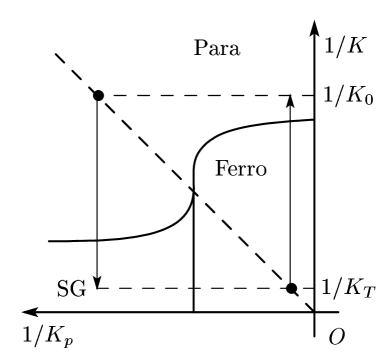
Figure 1: The processes of eq. (16) drawn as two arrows on the phase diagram. The solid curves are the phase boundaries and the dashed line of $45^{\mathrm{o}}$ represents the NL.

We can establish another type of non-equilibrium relation following Ozeki [18]. We consider a non-equilibrium relaxation of the local magnetization $\langle S_{i}(T)\rangle_{K_{0}\rightarrow K_{T}}^{\mathrm{F}}$, where F means that the initial state is $\mathbf{S}_{0}=(+1,+1,\cdots,+1)$. We evaluate the time evolution of the local magnetization as

$$\langle S_{i}(T)\rangle_{K_{0}\rightarrow K_{T}}^{\mathrm{F}}=\sum_{\{\mathbf{S}\}}S_{i}(T)\mathrm{e}^{\Delta tM(\mathbf{S}_{n}|\mathbf{S}_{n-1};t_{n})}\cdots\mathrm{e}^{\Delta tM(\mathbf{S}_{1}|\mathrm{F};t_{1})},$$ (17)

where $\Delta t(\ll 1)$ is the unit time interval and $M(\mathbf{S}|\mathbf{S}^{\prime};t_{n})$ is the transition rate from state $\mathbf{S}^{\prime}$ to state $\mathbf{S}$ following the master equation. The initial condition F is different from the case of non-equilibrium relations, where the equilibrium distribution is assumed initially.

Let us apply the gauge transformation to $\langle S_{i}(T)\rangle_{K_{0}\rightarrow K_{T}}^{\mathrm{F}}$ [18],

$$\langle S_{i}(T)\rangle_{K_{0}\rightarrow K_{T}}^{\mathrm{F}}=\sum_{\{\mathbf{S}\}}S_{i}\sigma_{i}(T)\mathrm{e}^{\Delta tM(\mathbf{S}_{n}|\mathbf{S}_{n-1};t_{n})}\cdots\mathrm{e}^{\Delta tM(\mathbf{S}_{1}|\sigma;t_{1})}.$$ (18)

The configurational average for $\langle S_{i}(T)\rangle_{K_{0}\rightarrow K_{T}}^{\mathrm{F}}$ is thus

$$\left[\langle S_{i}(T)\rangle_{K_{0}\rightarrow K_{T}}^{\mathrm{F}}\right]_{K_{p}}$$

$$\quad=\sum_{\{\tau_{ij}\}}\sum_{\{\mathbf{S}\}}S_{i}(T)\sigma_{i}\frac{1}{(2\cosh K_{p})^{N_{B}}}\prod_{\langle ij\rangle}\mathrm{e}^{K_{p}\tau_{ij}\sigma_{i}\sigma_{j}}\mathrm{e}^{\Delta tM(\mathbf{S}_{n}|\mathbf{S}_{n-1};t_{n})}\cdots\mathrm{e}^{\Delta tM(\mathbf{S}_{1}|\sigma;t_{1})}.$$ (19)

If we set $K_{p}=K_{0}$ and take the summation over all configurations of $\sigma$, we obtain

$$\left[\langle S_{i}(T)\rangle_{K_{0}\rightarrow K_{T}}^{\mathrm{F}}\right]_{K_{0}}=\sum_{\{\tau_{ij}\}}\frac{Z(K_{0};\{\tau_{ij}\})}{2^{N}(2\cosh K_{0})^{N_{B}}}\langle S_{i}(T)S_{i}(0)\rangle_{K_{0}\rightarrow K_{T}}.$$ (20)

Since the autocorrelation function is gauge-invariant, the right-hand side can be shown to be the configurational average using the same method as in eq. (10)[18],

$$\left[\langle S_{i}(T)\rangle_{K_{0}\rightarrow K_{T}}^{\mathrm{F}}\right]_{K_{0}}=\left[\langle S_{i}(0)S_{i}(T)\rangle_{K_{0}\rightarrow K_{T}}\right]_{K_{0}}.$$ (21)

Similarly we can prove that the autocorrelation function with the exponentiated work satisfies

$$\left[\langle S_{i}(T)\mathrm{e}^{-\beta W}\rangle_{K_{T}\rightarrow K_{0}}^{\mathrm{F}}\right]_{K_{T}}=\left[\langle S_{i}(0)S_{i}(T)\mathrm{e}^{-\beta W}\rangle_{K_{T}\rightarrow K_{0}}\right]_{K_{T}}.$$ (22)

Comparison of eqs. (16) (with $K_{T}$ and $K_{0}$ exchanged), (21) and (22) reveals

$$\left[\langle S_{i}(T)\rangle_{K_{0}\rightarrow K_{T}}^{\mathrm{F}}\right]_{K_{0}}=\left[\langle S_{i}(T)\mathrm{e}^{-\beta W}\rangle_{K_{T}\rightarrow K_{0}}^{\mathrm{F}}\right]_{K_{T}}\left(\frac{2\cosh K_{T}}{2\cosh K_{0}}\right)^{N_{B}}.$$ (23)

3.2 Gauge-non-invariant quantities

As a typical gauge-non-invariant quantity, we choose $S_{i}(T)$ for $O$ in eq. (5). After the configurational average, we have

$$\left[\left\langle S_{i}(T)\mathrm{e}^{-\beta W}\right\rangle_{K_{0}\rightarrow K_{T}}\right]_{K_{p}}=\left[\langle S_{i}\rangle_{K_{T}}\frac{Z(K_{T};\{\tau_{ij}\})}{Z(K_{0};\{\tau_{ij}\})}\right]_{K_{p}}.$$ (24)

Gauge transformation for the right-hand side in this equation yields

$$\left[\langle S_{i}\rangle_{K_{T}}\frac{Z(K_{T};\{\tau_{ij}\})}{Z(K_{0};\{\tau_{ij}\})}\right]_{K_{p}}=\sum_{\{\tau_{ij}\}}\frac{Z(K_{T};\{\tau_{ij}\})}{Z(K_{0};\{\tau_{ij}\})}\langle S_{i}\rangle_{K_{T}}\sigma_{i}\prod_{\langle ij\rangle}\frac{\mathrm{e}^{K_{p}\tau_{ij}\sigma_{i}\sigma_{j}}}{2\cosh K_{p}}.$$ (25)

As usual, we sum both sides of this equation over all the possible configurations of $\sigma$ and divide the obtained quantity by $2^{N}$ to find

$$\left[\langle S_{i}\rangle_{K_{T}}\frac{Z(K_{T};\{\tau_{ij}\})}{Z(K_{0};\{\tau_{ij}\})}\right]_{K_{p}}=\sum_{\{\tau_{ij}\}}\frac{Z(K_{p};\{\tau_{ij}\})}{2^{N}(2\cosh K_{p})^{N_{B}}}\langle S_{i}\rangle_{K_{T}}\langle\sigma_{i}\rangle_{K_{p}}\frac{Z(K_{T};\{\tau_{ij}\})}{Z(K_{0};\{\tau_{ij}\})}.$$ (26)

The following relation can also be derived in a similar manner,

$$\left[\langle S_{i}\rangle_{K_{0}}\right]_{K_{p}}=\sum_{\{\tau_{ij}\}}\frac{Z(K_{p};\{\tau_{ij}\})}{2^{N}(2\cosh K_{p})^{N_{B}}}\langle S_{i}\rangle_{K_{0}}\langle\sigma_{i}\rangle_{K_{p}}.$$ (27)

Setting $K_{p}=K_{0}$ in eq. (26) and $K_{p}=K_{T}$ in eq. (27), we find a relation

$$\left[\langle S_{i}\rangle_{K_{T}}\frac{Z(K_{T};\{\tau_{ij}\})}{Z(K_{0};\{\tau_{ij}\})}\right]_{K_{0}}=\left[\langle S_{i}\rangle_{K_{0}}\right]_{K_{T}}\left(\frac{2\cosh K_{T}}{2\cosh K_{0}}\right)^{N_{B}}.$$ (28)

Thus a non-equilibrium relation results,

$$\left[\langle S_{i}(T)\mathrm{e}^{-\beta W}\rangle_{K_{0}\rightarrow K_{T}}\right]_{K_{0}}=\left[\langle S_{i}\rangle_{K_{0}}\right]_{K_{T}}\left(\frac{2\cosh K_{T}}{2\cosh K_{0}}\right)^{N_{B}}.$$ (29)

The same method yields

$$\left[\langle S_{0}(T)S_{r}(T)\mathrm{e}^{-\beta W}\rangle_{K_{0}\rightarrow K_{T}}\right]_{K_{0}}=\left[\langle S_{0}S_{r}\rangle_{K_{0}}\right]_{K_{T}}\left(\frac{2\cosh K_{T}}{2\cosh K_{0}}\right)^{N_{B}}.$$ (30)

Equations (29) and (30) relate the equilibrium physical quantities evaluated away from the NL (the right-hand sides) with other quantities measured by non-equilibrium processes from a point on the NL to another point away from the NL (the left-hand sides) as depicted in Fig. 2.

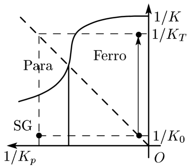
Figure 2: Equations (29) and (30) relate equilibrium physical quantities evaluated at a point $(1/K_{0},1/K_{T})$ (the lower-left dot in each panel) with other physical quantities evaluated by non-equilibrium processes shown in an arrow. The lower-left dot is in the spin glass phase whereas the corresponding arrow is in the ferromagnetic phase.

4 Summary

We have studied applications of non-equilibrium relations, typically the Jarzynski equality, to the context of spin glasses with gauge symmetry. It has been shown that the configurational average greatly simplifies a number of expressions appearing in non-equilibrium relations. In particular, the right-hand side of the Jarzynski equality, usually written as $\mathrm{e}^{-\beta\Delta F}$, reduces to a trivial analytic function of the initial and final temperatures, which has been used to prove a simple lower bound on the work. Many identities have also been derived for gauge-invariant and gauge-non-invariant quantities, which relate physical quantities measured at quite different environments. Most notably, the equilibrium values of the single-site magnetization and correlation function have been proved to be proportional to the non-equilibrium values of the corresponding quantities measured at different parts of the phase diagram. This result may possibly be useful to numerically evaluate equilibrium physical quantities in the spin glass phase from non-equilibrium calculations away from the spin glass phase with the aid of annealed importance sampling or population annealing method [7, 8, 9].

References

• [1] K. Binder, and A. P. Young: Rev. Mod. Phys. 58 (1986) 801.
• [2] A. P. Young (ed.): Spin Glasses and Random Fields (World Scientific, Singapore, 1997).
• [3] N. Kawashima, and H. Rieger: in Frustrated Spin Systems, ed. T. H. Diep (World Scientific, Singapore, 2004).
• [4] M. MΓ©zard, G. Parisi and M. A. Virasoro: Spin Glass Theory and Beyond (World Scientific, Singapore, 1987).
• [5] R. H. Swendsen, and J. S. Wang: Phys. Rev. Lett. 58 (1987) 56.
• [6] K. Hukushima, and K. Nemoto: J. Phys. Soc. Jpn. 65 (1996) 1604.
• [7] R. M. Neal: Statistics and Computing, 11 (2001) 125.
• [8] Y. Iba: Trans. Jpn. Soc. Artif. Intel. 16 (2001) 279.
• [9] K. Hukushima, and Y. Iba: AIP. Conf. Proc. 690 (2003) 200.
• [10] Y. Ozeki and N. Ito: J. Phys. A: Math. Theor. 40 (2007) R149.
• [11] C. Jarzynski: Phys. Rev. Lett. 78 (1997) 2690.
• [12] C. Jarzynski: Phys. Rev. E 56 (1997) 5018.
• [13] G. E. Crooks: J. Stat. Phys. 90 (1998) 1481.
• [14] G. E. Crooks: Phys. Rev. E 60 (1999) 2721.
• [15] G. E. Crooks: Phys. Rev. E 61 (2000) 2361.
• [16] H. Nishimori: Prog. Theor. Phys. 66 (1981) 1169.
• [17] H. Nishimori: Statistical Physics of Spin Glasses and Information Processing: An Introduction (Oxford Univ. Press, Oxford, 2001).
• [18] Y. Ozeki: J. Phys. A: Math. Gen. 28 (1995) 3645.