Exact Microtheoretical Approach to Calculation of Optical Properties of Ultralow Dimensional Crystals

Abstract

The main problem in theoretical analysis of structures with strong confinement is the fact that standard mathematical tools: differential equations and Fourier’s transformations are no longer applicable. In this paper we have demonstrated that method of Green’s functions can be successfully used on low-dimension crystal samples, as a consequence of quantum size effects. We can illustrate modified model through the prime cubic structure molecular crystal: bulk and ultrathin film. Our analysis starts with standard exciton Hamiltonian with definition of commutative Green’s function and equation of motion. We have presented detailed procedure of calculations of Green’s functions, and further dispersion law, distribution of states and relative permittivity for bulk samples. After this, we have followed the same procedures for obtaining the properties of excitons in ultra-thin films. The results have been presented graphically. Besides modified method of Green’s functions we have shown that the exciton energy spectrum is discrete in film structures (with number of energy levels equal to the number of atomic planes of the film). Compared to the bulk structures, with continual absorption zone, in film structures exist resonant absorption peaks. With increased film thickness differences between bulk and film vanish.

1 Introduction

Interest in exciton subsystem studies appeared due to the fact that excitons are responsible for dielectric, optical (absorption, dispersion of light, luminescence), photoelectric and other properties of crystals [1$-$3]. Studies of excitons in crystalline subsystems culminated with laser invention.

In recent years theoretical investigations of quasi-two-dimensional exciton subsystems (nanostructures) were intensified, especially in the field of thin films, not only to obtain fundamental information regarding dielectric properties of these materials but also because of their wide practical use (nanoelectronics, optoelectronic [4$-$6], light energy conversion [9,10]…). What is unique for these structures is that they have changed properties compared to their bulk analogues [6$-$8].

We studied the basic physical characteristics of ultrathin dielectrics $-$ molecular crystalline nanofilms [11,12], which could be used as surface layers for protection of electronic components or as special light filters.

This paper analyzes the influence of border-film structure on the energy spectrum of excitons (exciton dispersion law). Special attention was paid to the presence and spatial distribution of localized exciton states. Optical properties of these dielectric films were also investigated (their dielectric permittivity was determined). Results obtained in this work were compared with the similar results for the case of ideal infinite crystals, in order to find most important differences between these two systems.

These analyzes may be conducted using methods of two-time, temperature-dependant Green’s functions that are often used in quantum theory of solid state [13$-$15]. With adequately incorporated statistics, this method is being successfully applied in calculations of microscopic and macroscopic, as well as balanced and non-balanced properties of crystals.

A question which justifiably arises is related to the mean of calculating Green’s functions, which are ”borrowed” from the quantum field theory and whose definition, i.e. usage, is based on variables with continuous spectra in unlimited (both direct and impulse) space!

This work proves that the method of Green’s functions may be successfully applied onto crystalline samples of such small dimensions that the quantum size effects are relevant [16]. In order to illustrate adaptation of this method, we will observe molecule crystal with a simple cubic structure: spatially unlimited (bulk) and strongly limited along one axis (ultra thin film). Our intention is to show a technique of application of Green’s function onto spatially limited systems, so we excluded from calculation all really existing parameters: more complex crystalline structure, changes in boundary film parameters etc.

2 Excitons in bulk-structures

The discussion of dielectric properties of an ideal (with no defects, vacancies, etc) unlimited molecular crystal will start with standard exciton Hamiltonian, which has following form in configuration space [1,15,17]:

$$H=H_{0}+\sum_{\vec{n}}\Delta_{\vec{n}}\,P_{\vec{n}}^{+}P_{\vec{n}}+\sum_{\vec{n},\vec{m}}X_{\vec{n}\vec{m}}\,P_{\vec{n}}^{+}P_{\vec{m}}+\sum_{\vec{n},\vec{m}}Y_{\vec{n}\vec{m}}\,P_{\vec{n}}^{+}P_{\vec{n}}P_{\vec{m}}^{+}P_{\vec{m}}\,,$$ (1)

where $P_{\vec{n}}^{+}$ and $P_{\vec{n}}$ represent creation and annihilation exciton operators at the node (site) $\vec{n}$ of the crystalline lattice. Quantity $\Delta_{\vec{n}}$ represents the energy of the exciton localized at the $\vec{n}$ node, while the quantities $X_{\vec{n},\vec{m}}$ and $Y_{\vec{n},\vec{m}}$ represent matrix elements of the exciton transfer from the node $\vec{n}$ to the node $\vec{m}$.

Properties of the model exciton system may be analyzed using commutation Paulian Green’s function [13,14,18]:

$$\Gamma_{\vec{n}\vec{m}}(t)\equiv\langle\langle P_{\vec{n}}(t)\mid P_{\vec{m}}^{+}(0)\rangle\rangle=\Theta(t)\,\langle\left[P_{\vec{n}}(t),\,P_{\vec{m}}^{+}(0)\right]\rangle\,,$$ (2)

which satisfies following equation of motion:

$$\mbox{i}\hbar\,\frac{d}{dt}\,\Gamma_{\vec{n}\vec{m}}(t) =\mbox{i}\hbar\,\delta(t)\,\langle\left[P_{\vec{n}}(t),\,P_{\vec{m}}^{+}(0)\right]\rangle+$$ (3)

$$+\Theta(t)\langle\left[P_{\vec{n}}(t),H\right]\,P_{\vec{m}}^{+}(0)-P_{\vec{m}}^{+}(0)\left[P_{\vec{n}}(t),H\right]\rangle\,.$$

Using commutation relations for Pauli operators [18,19]:

$$\begin{array}[]{c}\displaystyle\left[P_{\vec{n}},P_{\vec{m}}^{+}\right]=\left(1-2P_{\vec{n}}^{+}P_{\vec{n}}\right)\,\delta_{\vec{n}\vec{m}}\,;\vspace*{1.0mm}\\ \displaystyle\left[P_{\vec{n}},P_{\vec{m}}\right]=\left[P_{\vec{n}},P_{\vec{m}}^{+}\right]=0\,;\;\;\;P_{\vec{n}}^{2}=\left(P_{\vec{n}}^{+}\right)^{2}=0\,,\end{array}$$ (4)

we obtain the equation of motion for Paulian Green’s function:

$$\mbox{i}\hbar\,\frac{d}{dt}\,\Gamma_{\vec{n}\vec{m}}(t) =\mbox{i}\hbar\,\delta(t)\delta_{\vec{n}\vec{m}}\left(1-2\langle P_{\vec{n}}^{+}P_{\vec{n}}\rangle\right)+$$

$$+\Delta_{\vec{n}}\,\Gamma_{\vec{n}\vec{m}}(t)+\sum_{\vec{l}}X_{\vec{n}\vec{l}}\,\Gamma_{\vec{l}\vec{m}}(t)-$$ (5)

$$-2\sum_{\vec{l}}X_{\vec{n}\vec{l}}\,\mathcal{T}_{\vec{n}\vec{n}\vec{l}\vec{m}}(t)+2\sum_{\vec{l}}Y_{\vec{n}\vec{l}}\,\mathcal{T}_{\vec{l}\vec{l}\vec{n}\vec{m}}(t)$$

expressed by $\mathcal{T}_{\vec{n}\vec{n}\vec{l}\vec{m}}(t)=\langle\langle P_{\vec{n}}^{+}(t)P_{\vec{n}}(t)P_{\vec{l}}(t)\mid P_{\vec{m}}^{+}(0)\rangle\rangle-$ Paulian Green’s function of the higher (third) order.

The basic problem with exciton theory is the fact that Pauli-operators $P^{+}$ and $P$ are not Bose or Fermi operators, but a certain hybrid of both with a kinematics described by expression (4), that is Fermian for one mode and Bosonian for different modes. For precise analysis of exciton systems, which encompass effects of inter-exciton interaction, simple replacing of Pauli-operators with Bose-operators is not enough. Therefore, in Hamiltonian (1), Pauli-operators are replaced by their exact Bosonian represents [20]:

$$P=\left[\sum_{\nu=0}^{\infty}\frac{(-2)^{\nu}}{(1+\nu)!}\left(B^{+}\right)^{\nu}B^{\nu}\right]^{\frac{1}{2}}B\,;$$

$$P^{+}=B^{+}\left[\sum_{\nu=0}^{\infty}\frac{(-2)^{\nu}}{(1+\nu)!}\left(B^{+}\right)^{\nu}B^{\nu}\right]^{\frac{1}{2}}\,;$$ (6)

$$P^{+}P=\sum_{\nu=0}^{\infty}\frac{(-2)^{\nu}}{(1+\nu)!}\left(B^{+}\right)^{\nu+1}B^{\nu+1}\,.$$

Our goal is to adapt Green’s function method to spatially quantum (discrete, not continuous) structures and to see the influence of spatial limits and disturbances of inner translational symmetry on changes of their macroscopic physical properties. Paulian Green’s functions from equation (7) will be therefore expressed using appropriate Bosonian Green’s functions on the basis of approximate expressions following from (6):

$$\begin{array}[]{c}\displaystyle P\approx B-B^{+}BB\,;\;\;\;P^{+}\approx B^{+}-B^{+}B^{+}B\,;\vspace*{1.0mm}\\ \displaystyle P^{+}P\approx B^{+}B-B^{+}B^{+}BB\,.\end{array}$$ (7)

By this we obtain:

$$\Gamma_{\vec{n}\vec{m}}(t)=\langle\langle P_{\vec{n}}(t)\mid P_{\vec{m}}^{+}(0)\rangle\rangle=\langle\langle B_{\vec{n}}(t)\mid B_{\vec{m}}^{+}(0)\rangle\rangle-$$

$$-\langle\langle B_{\vec{n}}(t)\mid B_{\vec{m}}^{+}(0)B_{\vec{m}}^{+}(0)B_{\vec{m}}(0)\rangle\rangle-\langle\langle B_{\vec{n}}^{+}(t)B_{\vec{n}}(t)B_{\vec{n}}(t)\mid B_{\vec{m}}^{+}(0)\rangle\rangle+$$ (8)

$$+\langle\langle B_{\vec{n}}^{+}(t)B_{\vec{n}}(t)B_{\vec{n}}(t)\mid B_{\vec{m}}^{+}(0)B_{\vec{m}}^{+}(0)B_{\vec{m}}(0)\rangle\rangle\,.$$

Further, by decoupling higher Green’s functions using known Bose-commutation relations:

$$\left[B_{\vec{k}},B_{\vec{l}}^{+}\right]=\delta_{\vec{k}\vec{l}}\,;\;\;\;\left[B_{\vec{k}},B_{\vec{l}}\right]=\left[B_{\vec{k}}^{+},B_{\vec{l}}^{+}\right]=0$$ (9)

and by introducing retarded (Bosonian) Green’s function:

$$\langle\langle B_{\vec{n}}(t)\mid B_{\vec{m}}^{+}(0)\rangle\rangle=G_{\vec{n}\vec{m}}(t)\,,$$ (10)

terms in expression (8) become:

$$\langle\langle B_{\vec{n}}(t)\mid B_{\vec{m}}^{+}(0)B_{\vec{m}}^{+}(0)B_{\vec{m}}(0)\rangle\rangle=\Theta(t)\langle\left[B_{\vec{n}},B_{\vec{m}}^{+}B_{\vec{m}}^{+}B_{\vec{m}}\right]\rangle =$$

$$=\Theta(t)\left(\langle\left(\delta_{\vec{n}\vec{m}}+B_{\vec{m}}^{+}B_{\vec{n}}\right)B_{\vec{m}}^{+}B_{\vec{m}}\rangle\right.-\left.\langle B_{\vec{m}}^{+}B_{\vec{m}}^{+}B_{\vec{m}}B_{\vec{n}}\rangle\right)=2G_{\vec{n}\vec{m}}(t)\mathcal{N}_{0}\,;$$

$$\langle\langle B_{\vec{n}}^{+}(t)B_{\vec{n}}(t)B_{\vec{n}}(t)\mid B_{\vec{m}}^{+}(0)\rangle\rangle=2G_{\vec{n}\vec{m}}(t)\mathcal{N}_{0}\,;$$ (11)

$$\;\;\;\langle\langle B_{\vec{n}}^{+}(t)B_{\vec{n}}(t)B_{\vec{n}}(t)\mid B_{\vec{m}}^{+}(0)B_{\vec{m}}^{+}(0)B_{\vec{m}}(0)\rangle\rangle=2R_{\vec{n}\vec{m}}(t)\,G_{\vec{n}\vec{m}}^{2}(t)\,,$$

where $\mathcal{N}_{0}$ is concentration of excitons, and $R_{\vec{n}\vec{m}}(t)$ is advanced Green’s function:

$$\begin{array}[]{l}\displaystyle\mathcal{N}_{0}=\langle B^{+}B\rangle=\frac{1}{N}\sum_{\vec{k}}\left(\mbox{ e}^{\hbar\omega_{{}_{0}}(\vec{k})/\theta}-1\right)^{-1};\\ \displaystyle R_{\vec{n}\vec{m}}(t)=\langle\langle B_{\vec{n}}^{+}(t)\mid B_{\vec{m}}(0)\rangle\rangle\,.\end{array}$$ (12)

When expressions (10) and (11) are substitued into eq.(8) we obtain final expression for Paulian Green’s function expressed using Bosonian Green’s functions:

$$\Gamma_{\vec{n}\vec{m}}(t)=\left(1-4\,\mathcal{N}_{0}\right)\,G_{\vec{n}\vec{m}}(t)+2R_{\vec{n}\vec{m}}(t)\,G_{\vec{n}\vec{m}}^{2}(t)+O(\mathcal{N}^{2})\,.$$ (13)

For Paulian Green’s functions of higher order ($\mathcal{T}_{\vec{a}\vec{a}\vec{b}\vec{c}}$) at the left side of Green’s function we simply replace Pauli operators by Bose-operators, and on the right side approximation (7) takes place. In this way it follows:

$$\mathcal{T}_{\vec{a}\vec{a}\vec{b}\vec{c}} =\langle\langle P_{\vec{a}}^{+}(t)P_{\vec{a}}(t)P_{\vec{b}}(t)\mid P_{\vec{c}}^{+}(0)\rangle\rangle=\langle\langle B_{\vec{a}}^{+}(t)B_{\vec{a}}(t)B_{\vec{b}}(t)\mid B_{\vec{c}}^{+}(0)\rangle\rangle-$$

$$-\langle\langle B_{\vec{a}}^{+}(t)B_{\vec{a}}(t)B_{\vec{b}}(t)\mid B_{\vec{c}}^{+}(0)B_{\vec{c}}^{+}(0)B_{\vec{c}}(0)\rangle\rangle=$$ (14)

$$=\mathcal{N}_{0}G_{\vec{b}\vec{c}}(t)+\mathcal{N}_{\vec{b}\vec{a}}G_{\vec{a}\vec{c}}(t)-2R_{\vec{a}\vec{c}}(t)\,G_{\vec{b}\vec{c}}(t)\,G_{\vec{a}\vec{c}}(t)+O(\mathcal{N}_{0}^{2})\,.$$

Expressions for $\Gamma_{\vec{n}\vec{m}}$, $\mathcal{T}_{\vec{n}\vec{n}\vec{l}\vec{m}}$ and $\mathcal{T}_{\vec{l}\vec{l}\vec{n}\vec{m}}$, which are expressed using Bosonian Green’s functions, are substituted in a equation of movement for Paulian Green’s function (5):

$$\mbox{i}\hbar\,\frac{d}{dt}\,\left[\left(1-4\,\mathcal{N}_{0}\right)\,G_{\vec{n}\vec{m}}(t)+2R_{\vec{n}\vec{m}}(t)\,G_{\vec{n}\vec{m}}^{2}(t)\right]=\mbox{i}\hbar\,\delta(t)\delta_{\vec{n}\vec{m}}\left(1-2\langle P_{\vec{n}}^{+}P_{\vec{n}}\rangle\right) +$$

$$+\Delta_{\vec{n}}\left[\left(1-4\mathcal{N}_{0}\right)\,G_{\vec{n}\vec{m}}(t)+2R_{\vec{n}\vec{m}}(t)\,G_{\vec{n}\vec{m}}^{2}(t)\right] +$$

$$+\sum_{\vec{l}}X_{\vec{n}\vec{l}}\left[\left(1-4\mathcal{N}_{0}\right)\,G_{\vec{l}\vec{m}}(t)+2R_{\vec{l}\vec{m}}(t)\,G_{\vec{l}\vec{m}}^{2}(t)\right] -$$ (15)

$$\;\;\;-2\sum_{\vec{l}}X_{\vec{n}\vec{l}}\left[\mathcal{N}_{0}G_{\vec{l}\vec{m}}(t)+\mathcal{N}_{\vec{l}\vec{n}}G_{\vec{n}\vec{m}}(t)\right.-\left.2R_{\vec{n}\vec{m}}(t)\,G_{\vec{l}\vec{m}}(t)\,G_{\vec{n}\vec{m}}(t)\right] +$$

$$\;\;\;+2\sum_{\vec{l}}Y_{\vec{n}\vec{l}}\left[\mathcal{N}_{0}G_{\vec{n}\vec{m}}(t)+\mathcal{N}_{\vec{n}\vec{l}}G_{\vec{l}\vec{m}}(t)\right.-\left.2R_{\vec{l}\vec{m}}(t)\,G_{\vec{n}\vec{m}}(t)\,G_{\vec{l}\vec{m}}(t)\right]\,$$ .

Since concentration of Frenkel’s excitons in molecular crystals is very low ($\mathcal{N}<1$ %), the equation above may be solved in the lowest approximation (this approximation is appropriate for neglecting anharmonic and nonlinear effects, i.e. non-calculating higher orders terms of exciton-exciton as well as exciton-phonon interactions, in agreement to estimates in [1$-$3,13$-$15]):

$$\langle P_{\vec{n}}^{+}P_{\vec{n}}\rangle\approx\langle B_{\vec{n}}^{+}B_{\vec{n}}\rangle=\mathcal{N}_{0}\approx 0\,;$$

$$\mathcal{N}_{\vec{a}\vec{b}}\approx 0\,;\;\;\;G\cdot G\approx 0\,;\;\;\;G\cdot R\approx 0\,.$$

”Decoupled” eq.(15) then obtains the following form:

$$\mbox{i}\hbar\frac{d}{dt}G_{\vec{n}\vec{m}}(t)=\mbox{i}\hbar\delta(t)\delta_{\vec{n}\vec{m}}+\Delta_{\vec{n}}G_{\vec{n}\vec{m}}(t)+\sum_{\vec{l}}X_{\vec{n}\vec{l}}G_{\vec{l}\vec{m}}(t)\,.$$ (16)

It is important to notice that this equation has to be obtained in the same form starting from effective Bosonian exciton Hamiltonian in harmonic approximation:

$$H_{\mbox{\scriptsize ex}}=\sum_{\vec{n}}\Delta_{\vec{n}}\,B_{\vec{n}}^{+}B_{\vec{n}}+\sum_{\vec{n},\vec{m}}X_{\vec{n}\vec{m}}\,B_{\vec{n}}^{+}B_{\vec{m}}\,,$$

and estimating Bosonian Green’s function (10):

$$G_{\vec{n}\vec{m}}(t)=\langle\langle B_{\vec{n}}(t)\mid B_{\vec{m}}^{+}(0)\rangle\rangle=\Theta(t)\,\langle\left[B_{\vec{n}}(t),\,B_{\vec{m}}^{+}(0)\right]\rangle\,,$$

with its equation motion:

$$\mbox{i}\hbar\,\frac{d}{dt}\,G_{\vec{n}\vec{m}}(t) =\mbox{i}\hbar\,\delta(t)\,\langle\left[B_{\vec{n}}(t),\,B_{\vec{m}}^{+}(0)\right]\rangle+$$

$$+\Theta(t)\langle\left[B_{\vec{n}}(t),H_{\mbox{\scriptsize ex}}\right]\,B_{\vec{m}}^{+}(0)-B_{\vec{m}}^{+}(0)\left[B_{\vec{n}}(t),H_{\mbox{\scriptsize ex}}\right]\rangle\,.$$

This (by time) differential equation (16) is solved using temporal Fourier’s transformation:

$$f_{\vec{a}\vec{b}}(t)=\int\displaylimits_{-\infty}^{+\infty}d\omega f_{\vec{a}\vec{b}}(\omega)\,\operatorname{e}^{-\mbox{\scriptsize i}\omega t}\,;\;\;\;\delta(t)=\frac{1}{2\pi}\int\displaylimits_{-\infty}^{+\infty}d\omega\,\operatorname{e}^{-\mbox{\scriptsize i}\omega t}\,,$$ (17)

and thus we obtain:

$$\hbar\omega G_{\vec{n}\vec{m}}(\omega)=\frac{\mbox{i}\hbar}{2\pi}\delta_{\vec{n}\vec{m}}+\Delta_{\vec{n}}G_{\vec{n}\vec{m}}(\omega)+\sum_{\vec{l}}X_{\vec{n}\vec{l}}G_{\vec{l}\vec{m}}(\omega)\,.$$ (18)

By using nearest neighbors approximation ($\vec{l}\rightarrow\vec{n}\pm\vec{\lambda}_{i}$): $\vec{n}\pm\vec{\lambda}_{1}=n_{x}\pm 1,n_{y},n_{z}$;   $\vec{n}\pm\vec{\lambda}_{2}=n_{x},n_{y}\pm 1,n_{z}$;  $\vec{n}\pm\vec{\lambda}_{3}=n_{x},n_{y},n_{z}\pm 1$ and taking into account that we are observing an ideal cubic structure, where exciton energy is the same at every node, and the energy transfer between neighbors is also the same: $\Delta_{\vec{a}}\equiv\Delta$;  $X_{\vec{a},\vec{a}\pm\vec{\lambda}_{i}}\equiv X_{i}$  $i\in\{x,y,z\}$, equation above is taking following form:

$$\hbar\omega\,G_{n_{x}n_{y}n_{z},m_{x}m_{y}m_{z}}(\omega) \equiv\hbar\omega\,G_{n_{x}n_{y}n_{z},\vec{m}}(\omega)=$$

$$=\frac{\mbox{i}\hbar}{2\pi}\delta_{n_{x}n_{y}n_{z},\vec{m}}+\Delta\,G_{n_{x}n_{y}n_{z},\vec{m}}(\omega)+$$

$$+X_{x}\left[G_{n_{x}+1,n_{y}n_{z};\vec{m}}(\omega)+G_{n_{x}-1,n_{y}n_{z};\vec{m}}(\omega)\right]+$$ (19)

$$+X_{y}\left[G_{n_{x}n_{y}+1,n_{z};\vec{m}}(\omega)+G_{n_{x}n_{y}-1,n_{z};\vec{m}}(\omega)\right]+$$

$$+X_{z}\left[G_{n_{x}n_{y}n_{z}+1;\vec{m}}(\omega)+G_{n_{x}n_{y}n_{z}-1;\vec{m}}(\omega)\right]\,.$$

Since the crystal is unlimited, when solving this linear differential equation we may use the full spatial Fourier’s transformation:

$$f_{\vec{a}\vec{b}}(\omega)=\frac{1}{N}\sum_{\vec{k}}f_{\vec{k}}(\omega)\operatorname{e}^{\mbox{\scriptsize i}\vec{k}(\vec{a}-\vec{b})}\,;\;\;\;\delta_{\vec{a}\vec{b}}=\frac{1}{N}\sum_{\vec{k}}\operatorname{e}^{\mbox{\scriptsize i}\vec{k}(\vec{a}-\vec{b})}\,.$$ (20)

By using these transformations and by composing the equation above, we obtain:

$$\hbar\omega\,G_{\vec{k}}(\omega) =\frac{\mbox{i}\hbar}{2\pi}+\Delta\,G_{\vec{k}}(\omega)+$$

$$+2\left(X_{x}\cos a_{x}k_{x}+X_{y}\cos a_{y}k_{y}+X_{z}\cos a_{z}k_{z}\right)\,G_{\vec{k}}(\omega)\,,$$ (21)

and from there we may express Green’s function:

$$G_{\vec{k}}(\omega) =\frac{\mbox{i}\hbar}{2\pi}\,\left[\hbar\omega-\Delta-\right.$$

$$-2\left.\left(X_{x}\cos a_{x}k_{x}+X_{y}\cos a_{y}k_{y}+X_{z}\cos a_{z}k_{z}\right)\right]^{-1}\equiv$$ (22)

$$\equiv\frac{\mbox{i}\hbar}{2\pi}\,\frac{1}{\hbar\omega-E_{\vec{k}}}\,.$$

We obtain the energy spectrum in a bulk monomolecular crystal [13,14] by calculating real part of the pole of this Green’s function:

$$E_{\vec{k}}=\Delta+2\left(X_{x}\cos a_{x}k_{x}+X_{y}\cos a_{y}k_{y}+X_{z}\cos a_{z}k_{z}\right)\,.$$ (23)

In order to perform comparison with dispersion law of excitons in the film, this expression will be written in a simpler ($X_{x}=X_{y}=X_{z}\equiv-|X|$, $a_{x}=a_{y}=a_{z}\equiv a$) and non-dimensional form:

$$\mathcal{E}_{\vec{k}}\equiv\frac{E_{\vec{k}}-\Delta}{|X|}=\mathcal{F}_{xy}+\mathcal{G}_{z}\,,$$ (24)

where

$$\mathcal{F}_{xy}=-2\left(\cos ak_{x}+\cos ak_{y}\right)\,;\;\;\;\mathcal{G}_{z}=-2\cos ak_{z}\,.$$

This dispersion law is shown in Figure 1, as a function of two-dimensional value $\mathcal{F}_{xy}$:

$$\mathcal{E}_{\vec{k}}=\mathcal{E}_{z}\left(\mathcal{F}_{xy}\right)\,,$$

It is clear that for $ak_{i}\in[0,+\pi]$, $i=x,y,z$ (the first Brilouin zone), these values are within the intervals:

$$\left.\begin{array}[]{r}\mathcal{F}_{xy}\in[-4,+4]\,;\vspace*{1.0mm}\\ \mathcal{G}_{z}\in[-2,+2]\,,\end{array}\,\right\}\,\Rightarrow\,\mathcal{E}_{\vec{k}}\in[-6,+6]\,.$$

The presence of permitted (continuous) energy levels is visible.

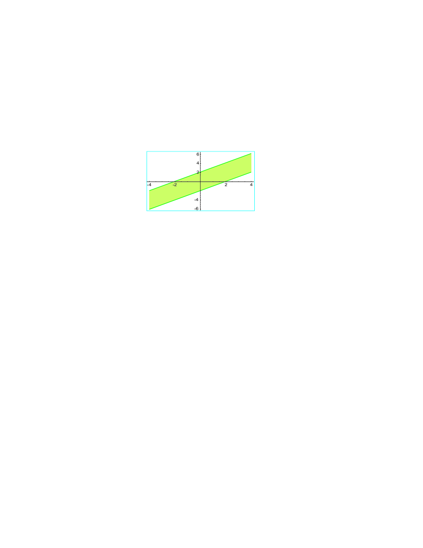
Figure 1: Exciton dispersion law of bulk crystal

Since molecular crystals are dielectric, it is essential to determine relative permittivity of these structures. The dynamic permittivity is defined by systems response to external perturbation [1,15,20], by expression:

$$\varepsilon^{-1}(\omega)=1-\frac{\pi S|X|}{\mbox{i}\hbar}\,\left[\,\Gamma(\omega)+\,\Gamma(-\omega)\right]\,,$$ (25)

where $S$ is a frequency property of a given crystal and external variable electromagnetic field. As it was mentioned before, in this (zero) approximation Paulian Green’s functions ($\Gamma$) are transforming into Bosonian ones ($G$), therefore:

$$\varepsilon^{-1}(\omega)=1-\frac{\pi S|X|}{\mbox{i}\hbar}\,\left[G(\omega)+G(-\omega)\right]\,.$$ (26)

Substituting (22) with (23) in (26) and by denoting $\displaystyle\frac{\hbar\omega}{|X|}\equiv|f|$ and $\displaystyle\frac{\Delta}{|X|}\equiv|p|$, we obtain the expression for dynamic permittivity in a bulk sample of monomolecular crystal (molecular crystal with simple cell):

$$\;\;\;\varepsilon_{\vec{k}}(\omega)=\left[1+S|X|\,\frac{E_{\vec{k}}}{(\hbar\omega)^{2}-E_{\vec{k}}^{2}}\right]^{-1}\equiv\left[1+S\,\frac{\mathcal{E}_{\vec{k}}+|p|}{|f|^{2}-\left(\mathcal{E}_{\vec{k}}+|p|\right)^{2}}\right]^{-1}.$$ (27)

Dependence of relative dynamic permittivity, expression (27), on reduced frequency (non-dimensional factor $\hbar\omega/\Delta$) of the external electromagnetic field is shown in Figure 2.

The presence of a single absorption zone is visible within certain boundary frequencies. This energy zone was calculated for two-dimension center of Brilouin’s zone ($k_{x}=k_{y}=0$;  $k_{z}=[0,\pi]$). For all other energies this crystal is transparent and has no spatial non-homogeneousness.

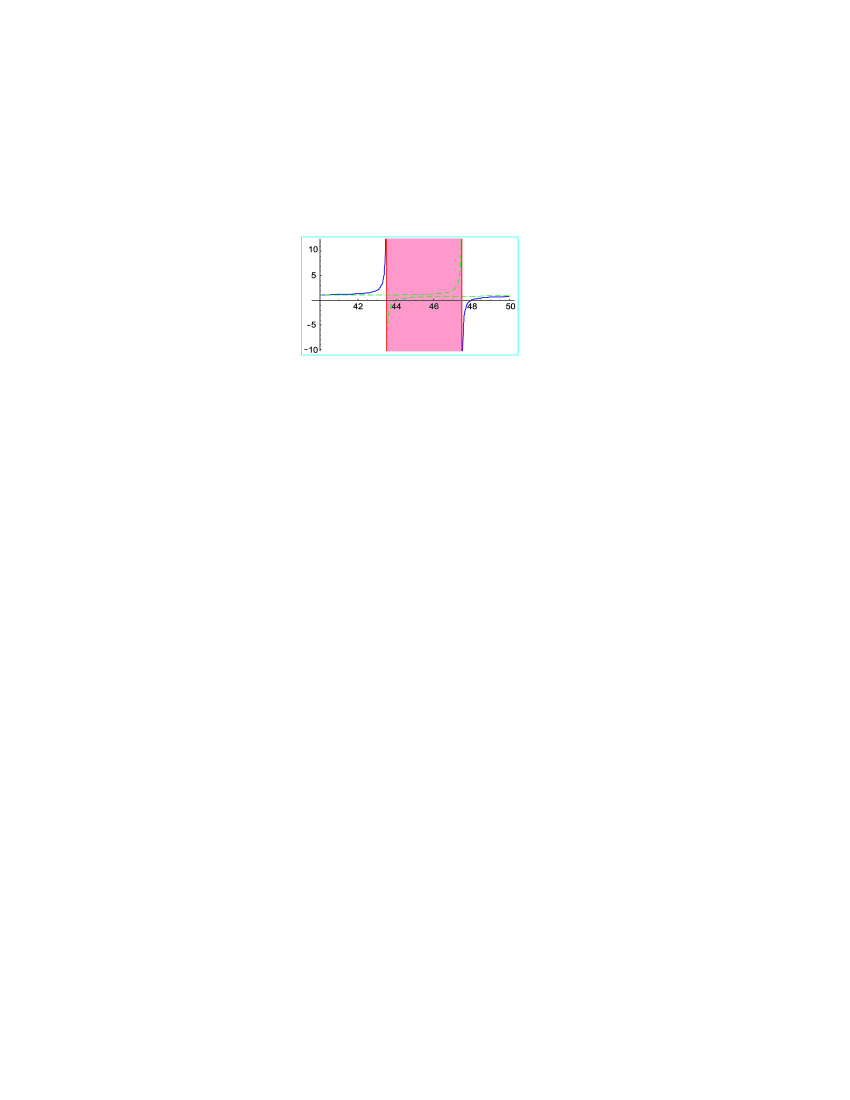
Figure 2: Relative permittivity of bulk crystal

3 Excitons in thin film-structures

Opposite to ideal unlimited structures, real crystals have no translation invariance property. The presence of certain boundary conditions is one of reasons for symmetry breaking [4$-$7]. Lets observe the ideal ultrathin film with simple cubic structure, made in the substrate i.e. by doping process. Here, by the term ”ideal”, we wanted to denote that there exist no breaking of inner crystal structure (no defects, ingredients, etc), and not as in no spatial limits. The film dimensions are such that it is unlimited in $XY$ planes, and in z-axis has final thickness ($L$). This means that this film has two unlimited boundary planes parallel to $XY$ planes, for $z=0$ and $z=L\equiv n_{z}$.

3.1 The model

The film-structure with primitive crystalline lattice (one molecule per elementary cell): monomolecular crystalline film, with specified parameters is shown in Figure 3.

Since boundary planes of the film are taken as being normal to $z$-axis, the index of parallel $XY$ planes $n_{z}$ has values $n_{z}=0,1,2,\,\ldots\,,\,N$ where $N\in[2,\,8]$ is for ultra thin films. Indices $n_{x}$ and $n_{y}$, determining position of a molecule in every $XY$ plane may have arbitrary whole-number values (practically from $-\infty$ to $+\infty$).

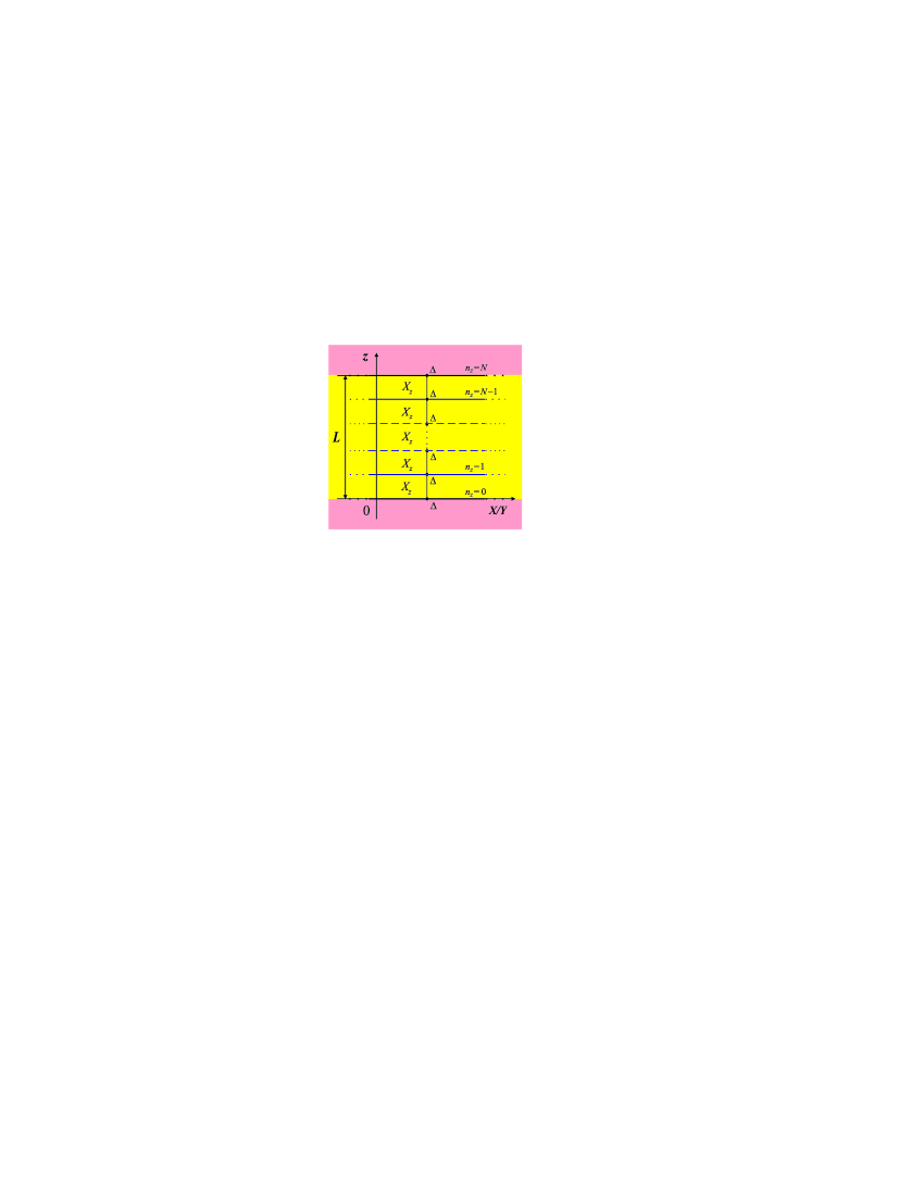
Figure 3: Cross-section of crystalline film-model

For calculating exciton energies in this film, we start from equation (19) on which, due to spatial limitations of the film at $z$-direction, we may apply partial spatial Fourier transformation:

$$\begin{array}[]{c}\displaystyle\delta_{\vec{n}\vec{m}}=\frac{1}{N_{x}N_{y}}\sum_{k_{x}k_{y}}\operatorname{e}^{ik_{x}a_{x}(n_{x}-m_{x})}\operatorname{e}^{ik_{y}a_{y}(n_{y}-m_{y})}\delta_{n_{z}m_{z}}\vspace*{1.0mm}\\ \displaystyle f_{\vec{n}\vec{m}}(\omega)=\frac{1}{N_{x}N_{y}}\sum_{k_{x}k_{y}}\operatorname{e}^{ik_{x}a_{x}(n_{x}-m_{x})}\operatorname{e}^{ik_{y}a_{y}(n_{y}-m_{y})}f_{n_{z}m_{z}}(k_{x},k_{y},\omega)\end{array}$$ (28)

(only along $x$ and $y$ directions). For expression shortening , it is convenient to introduce markings $G_{n_{z}m_{z}}(k_{x},k_{y},\omega)\equiv G_{n_{z}m_{z}}$. For $\displaystyle X_{x}=X_{y}=X_{z}\equiv-\left|X\right|$, $\displaystyle a_{x}=a_{y}=a_{z}\equiv a$ and $\displaystyle\mathcal{K}=\frac{i\hbar}{2\pi\left|X\right|}\delta_{n_{z},m_{z}}$, we obtain:

$$G_{n_{z}-1,m_{z}}+\varrho\,G_{n_{z}m_{z}}+G_{n_{z}+1,m_{z}}=\mathcal{K}\delta_{n_{z},m_{z}}\,,$$ (29)

where denotation is introduced:

$$\varrho =\frac{\hbar\omega-\Delta}{\left|X\right|}+2\left(\cos ak_{x}+\cos ak_{y}\right)\equiv$$

$$\equiv\frac{E_{\vec{k}}-\Delta}{\left|X\right|}-\mathcal{F}_{xy}\equiv\mathcal{E}_{\vec{k}}-\mathcal{F}_{xy}$$ (30)

(the quantity $\mathcal{F}_{xy}$ is defined in expression (24), while $\mathcal{E}_{\vec{k}}$ i.e. $E_{\vec{k}}$ which express a possible energy of excitons in films, will be calculated latter).

Equation (29) is in fact a system of $N+1$ nonhomogeneous algebraic differential equations with (starting boundary) conditions: $G_{n_{z},m_{z}}=0$, for $n_{z}<0$ and $n_{z}>N+1$:

$$\varrho\,G_{0}+G_{1} =\mathcal{K}_{0}$$

$$G_{0}+\varrho\,G_{1}+G_{2} =\mathcal{K}_{1}$$

$$G_{1}+\varrho\,G_{2}+G_{3} =\mathcal{K}_{2}$$

$$\cdots\;\;\;\;\cdots\;\;\;\;\cdots\; \;\;\;\;\cdots$$

$$G_{n_{z}-2}+\varrho\,G_{n_{z}-1}+G_{n_{z}} =\mathcal{K}_{n_{z}-1}$$

$$G_{n_{z}-1}+\varrho\,G_{n_{z}}+G_{n_{z}+1} =\mathcal{K}_{n_{z}}$$ (31)

$$G_{n_{z}}+\varrho\,G_{n_{z}+1}+G_{n_{z}+2} =\mathcal{K}_{n_{z}+1}$$

$$\cdots\;\;\;\;\;\;\;\;\;\cdots\;\;\;\;\;\;\;\;\;\cdots\;\;\; \;\;\;\;\;\;\cdots$$

$$G_{N-3}+\varrho\,G_{N-2}+G_{N-1} =\mathcal{K}_{N-2}$$

$$G_{N-2}+\varrho\,G_{N-1}+G_{N} =\mathcal{K}_{N-1}$$

$$G_{N-1}+\varrho\,G_{N} =\mathcal{K}_{N}$$

where is describe: $G_{n_{z}}\equiv G_{n_{z}m_{z}}$ and $\mathcal{K}\delta_{n_{z},m_{z}}\equiv\mathcal{K}_{n_{z}}$, because $m_{z}$ is blinding index.

3.2 Dispersion law

In order to find exciton energies, we need poles of Green’s functions, which are obtained when a determinant of a system (31) is equalized with zero, i.e.

$$D_{N+1}(\varrho)=\left|\begin{array}[]{ccccccccc}\varrho&1&0&0&\;\cdots&0&0&0&0\\ 1&\varrho&1&0&\cdots&0&0&0&0\\ 0&1&\varrho&1&\cdots&0&0&0&0\\ &&&&&&&&\\ \cdot&\cdot&\cdot&\cdot&\ddots&\cdot&\cdot&\cdot&\cdot\\ &&&&&&&&\\ 0&0&0&0&\cdots&1&\varrho&1&0\\ 0&0&0&0&\cdots&0&1&\varrho&1\\ 0&0&0&0&\;\cdots&0&0&1&\varrho\end{array}\right|_{N+1}\equiv 0\,,$$ (32)

and this determinant is actually a note for Chebyshev’s polynomials of second kind (and ($N+1$)-th order) [21,22]:

$$D_{N+1}(\varrho)\equiv\mathcal{C}_{N+1}(\varrho)=\varrho\,\mathcal{C}_{N}(\varrho)-\mathcal{C}_{N-1}(\varrho)\,.$$ (33)

The condition $D_{N+1}(\varrho)=0$ is reduced to $\mathcal{C}_{N+1}(\varrho)=0$ and is satisfied by $N+1$ solutions in form:

$$\varrho_{\nu}=-2\,\cos\frac{\nu\,\pi}{N+2}\,;\;\;\;\nu=1,2,\ldots,N+1\,.$$ (34)

Using this and replacing equation (30) we find:

$$E_{k_{x}k_{y}}(\nu)=\Delta-2|X|\left(\cos ak_{x}+\cos ak_{y}+\cos\frac{\pi\nu}{N+2}\right)\,.$$ (35)

In order to compare with dispersion law of excitons in a bulk we will write this expression in more simple, non-dimensional form ($\varrho_{\nu}=-2\cos a_{z}k_{z}(\mu)$):

$$\mathcal{E}_{k_{x}k_{y}}(\nu)=\mathcal{F}_{xy}+\mathcal{G}_{z}(\nu)\,;\;\;\;\mathcal{G}_{z}(\nu)\equiv\frac{1}{2}\left[1-\cos a_{z}k_{z}(\nu)\right]\,.$$ (36)

Previous expression represents the dispersion law of excitons of ideal monomolecular film and has the same form as the expression (24) obtained for corresponding ideal unlimited structures, with difference that in (24) $k_{z}$ is practically continuous variable (interval $[0,\pi/a]$) as $k_{x}$ and $k_{y}$, while here is discrete and is given by expression:

$$k_{z}(\nu)=\frac{\pi}{a}\frac{\nu}{N+2}\,;\;\;\;\nu=1,2,\,\ldots\,,N+1\,.$$ (37)

Graphical representation of dispersion law is given on Figure 4, showing possible exciton energies in ideal five-layer monomolecular film (full lines) together with bulk boundaries (dotted lines). Same as for corresponding bulk crystalline structures, we will use ordinate for values of reduced non-dimensional energies $\displaystyle\mathcal{E}_{\nu}$, depending on two-dimensional function $\mathcal{F}_{xy}$, for which is used graph abscissa.

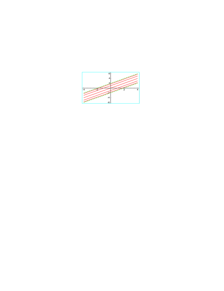
Figure 4: Exciton energies of molecular film

These analyzes have shown significant differences regarding dispersion law for excitons in spatially strongly limited systems (nanofilm-structures) as strictly result of border presence of these structures, in which energy spectra is highly discrete and have two gaps. Sizes of gaps depends on film thickness and decrease rapidly with its increase.

3.3 Spectral weights

In order to find certain Green’s function we will start from the system of equations (29), which is now suitable to represent in the operator form:

$$\hat{\mathcal{D}}_{N+1}\hat{\mathcal{G}}_{N+1}=\hat{\mathcal{K}}_{N+1}\;\;\Longrightarrow\;\;\hat{\mathcal{G}}_{N+1}=\hat{\mathcal{D}}_{N+1}^{-1}\hat{\mathcal{K}}_{N+1}\,,$$ (38)

where: $\hat{\mathcal{D}}_{N+1}$ is a matrix corresponding to the determinant of system $D_{N+1}$, $\hat{\mathcal{G}}_{N+1}$ and $\hat{\mathcal{K}}_{N+1}$ are vectors of Green’s functions and Kronecker’s delta symbols:

$$\begin{array}[]{r}\displaystyle\tilde{\mathcal{G}}_{N+1}=\left(\begin{array}[]{c}G_{0,m_{z}}\\ G_{1,m_{z}}\\ \;.\\ \;.\\ \;.\\ G_{n_{z},m_{z}}\;.\\ \;.\\ \;.\\ G_{N,m_{z}}\end{array}\right);\;\;\;\displaystyle\tilde{\mathcal{K}}_{N+1}=-\frac{i\hbar}{2\pi\left|X\right|}\left(\begin{array}[]{c}\delta_{0,m_{z}}\\ \delta_{1,m_{z}}\\ \;.\\ \;.\\ \;.\\ \delta_{n_{z},m_{z}}\;.\\ \;.\\ \;.\\ \delta_{N,m_{z}}\end{array}\right).\end{array}$$ (39)

Since the inverse matrix $\hat{\mathcal{D}}_{N+1}^{-1}$ may be expressed through adjunct matrix, whose elements $D_{ik}$ are cofactors of elements $d_{ik}$ from the direct matrix, we may write:

$$G_{n_{z},m_{z}} =\frac{1}{\mathcal{D}_{N+1}}\sum_{q}D_{n_{z},q}K_{q,m_{z}}=$$

$$=-\frac{1}{\mathcal{D}_{N+1}}\frac{i\hbar}{2\pi\left|X\right|}\sum_{q}D_{n_{z},q}\delta_{q,m_{z}}=$$ (40)

$$=-\frac{i\hbar}{2\pi\left|X\right|}\frac{D_{n_{z},m_{z}}}{\mathcal{D}_{N+1}}\,.$$

Cofactor $D_{n_{z},m_{z}}$ calculation is based on knowing the system determinant $D_{N+1}$.

Since for the equilibrium processes within system are important only diagonal Green’s functions $G_{n_{z};n_{z}}\equiv G_{n_{z}}$, calculating cofactors $D_{n_{z},m_{z}}\equiv D_{n_{z}}$ is significantly simplified. It turns out that they are equal to the product of two auxiliary determinants:

$$D_{n_{z}}=\mathcal{C}_{n_{z}}\mathcal{C}_{N-n_{z}}\,,$$ (41)

where $\mathcal{C}_{n_{z}-1}$ and $\mathcal{C}_{N-n_{z}}$ are corresponding Chebyshev’s polynomials of second kind. Therefore, Green’s function of the ideal film is:

$$G_{n_{z}}=\frac{i\hbar}{2\pi\left|X\right|}\frac{\mathcal{C}_{n_{z}}\mathcal{C}_{N-n_{z}}}{\mathcal{C}_{N+1}}\,.$$ (42)

These Green’s functions are multipolar, since denominator consists of a polynomial $\mathcal{C}_{N+1}$ of $N+1$-th order. Therefore factorization on simple poles must be performed [21]:

$$G_{n_{z}}=-\frac{i\hbar}{2\pi|X|}\sum_{\nu=1}^{N+1}\frac{g_{n_{z};n_{z}}(\varrho_{\nu})}{\varrho-\varrho_{\nu}}\,.$$ (43)

Spectral weights $g_{n_{z};n_{z}}(\varrho_{\nu})\equiv g_{n_{z}}^{\nu}$ then may be expressed using:

$$g_{n_{z}}^{\nu}=\frac{\mathcal{C}_{n_{z}}(\varrho_{\nu})\mathcal{C}_{N-n_{z}}(\varrho_{\nu})}{\displaystyle\left.\frac{d}{d\varrho}\mathcal{C}_{N+1}(\varrho)\right|_{\varrho=\varrho(\nu)}}\,.$$ (44)

Using the rule for derivative of determinant we obtain:

$$\left[\frac{d}{d\varrho}\mathcal{C}_{N+1}(\varrho)\right]_{\varrho=\varrho_{\nu}}=\sum_{i=1}^{N+1}\mathcal{C}_{i-1}(\varrho_{\nu})\mathcal{C}_{N+1-i}(\varrho_{\nu})=$$

$$=\sum_{i=1}^{N+1}\frac{\sin i\xi_{\nu}\sin(N+2-i)\xi_{\nu}}{\sin^{2}\xi_{\nu}}=$$ (45)

$$=\frac{\sin^{2}(n_{z}+1)\xi_{\nu}}{\displaystyle\sum\displaylimits_{i=1}^{N+1}\sin^{2}i\xi_{\nu}}\,;\;\;\;\xi_{\nu}=\frac{\pi\nu}{N+2}\,,$$

and spectral weights became:

$$g_{n_{z}}^{\nu}=\frac{2}{N+2}\sin^{2}\left[(n_{z}+1)\frac{\pi\nu}{N+2}\right]\,.$$ (46)

The spectral weights of Green’s functions are squares of the modules of the wave function of excitons [1$-$3,13$-$15] and enable determination of spatial distribution, i.e. probability to find excitons with certain energies per layers of crystalline film. This is in fact the spatial distribution of probability to find certain energy state of excitons.

Numerically calculated, values of reduced energies and corresponding spectrum functions (spatial distribution of probability) for four-layered film ($N=4$, where $k_{x}=k_{y}=0$) are shown in the table.

Table 1. shows spatial distribution of exciton energies occurrence probabilities in ideal monomolecular film.

Reduced	ULTRATHIN FILM
relative	a t o m i c   p l a n e
ENERGY	$\displaystyle\begin{array}[]{c}\mbox{\footnotesize upper}\vspace*{-1.5mm}\\ \mbox{\footnotesize boundary}\end{array}$	$\displaystyle\begin{array}[]{c}\mbox{\footnotesize first}\vspace*{-1.5mm}\\ \mbox{\footnotesize inner}\end{array}$	$\displaystyle\begin{array}[]{c}\mbox{\footnotesize central}\vspace*{-1.5mm}\\ \mbox{\footnotesize(inner)}\end{array}$	$\displaystyle\begin{array}[]{c}\mbox{\footnotesize last}\vspace*{-1.5mm}\\ \mbox{\footnotesize inner}\end{array}$	$\displaystyle\begin{array}[]{c}\mbox{\footnotesize lower}\vspace*{-1.5mm}\\ \mbox{\footnotesize boundary}\end{array}$
$-$1,73205	0,08333	0,25000	0,33333	0,25000	0,08333
$-$1,00000	0,25000	0,25000	0,00000	0,25000	0,25000
0,00000	0,33333	0,00000	0,33333	0,00000	0,33333
1,00000	0,25000	0,25000	0,00000	0,25000	0,25000
1,73205	0,08333	0,25000	0,33333	0,25000	0,08333

Table 1: Exciton probabilities in the ideal four-layered film

This table shows that for one certain energy, probability of exciton occurrence per all layers is equal to one, and that probability per one layer for all energies is also equal to one, i.e.

$$\sum_{n_{z}=0}^{N}g_{n_{z}}^{\nu}=1\,;\;\;\;\sum_{\nu=1}^{N+1}g_{n_{z}}^{\nu}=1\,.$$ (47)

3.4 The permittivity

While determining dynamic permittivity of crystalline film, the formula by Dzyaloshinski and Pitaevski [20] may also be used in the same form (26) in which was used for calculating permittivity of corresponding bulk structures, with difference that in this case permittivity depends on a film layer $n_{z}$, i.e:

$$\varepsilon_{n_{z}}^{-1}(\omega)=1-\frac{\pi\,S\,|X|}{\mbox{i}\,\hbar}\,\left[G_{n_{z}}(\omega)+G_{n_{z}}(-\omega)\right]\,.$$ (48)

Since starting Hamiltonian was taken in harmonic approximation, ignoring (small) members of exciton-phonon interaction [1,6,15], permittivity tensor has the real elements only. It is led to that all elements of permittivity tensor in one crystalline plane parallel to boundary planes are mutually equivalent, i.e. they depend on plane position ($n_{z}\in[0,N]$).

Substituting expression for Green’s functions (43) to (46), we obtain expression for the relative dynamic permittivity tensor elements in direction normal to boundary planes in form:

$$\varepsilon_{n_{z}}^{-1}=1-\frac{S}{2}\sum_{\nu=1}^{N+1}\sum_{s=+,-}\frac{g_{n_{z}}^{\nu}}{\varrho_{s}-\varrho_{\nu}}\,,$$ (49)

where: $\displaystyle\varrho_{\pm}=\mp|f|-|p|-\mathcal{F}_{xy}$, and after arranging the expression we finally follow:

$$\varepsilon_{n_{z}}(\omega)=\left[1+S\,\sum_{\nu=1}^{N+1}g^{\nu}_{n_{z}}\frac{\varrho_{\nu}-|p|+\mathcal{F}_{xy}}{|f|^{2}-\left(\varrho_{\nu}-|p|+\mathcal{F}_{xy}\right)^{2}}\right]^{-1}\,.$$ (50)

Figures 5 a-c show a dependence of dynamical permittivity ($\varepsilon$) on reduced relative energy, i.e. the frequency of external electromagnetic field ($f\equiv\hbar\omega/|X|$) for four-layered monomolecular film. Dependence was calculated for plane center of the Brilouin’s zone ($k_{x}=k_{y}=0$), but individually per atom planes (parallel boundary areas) of crystalline film, that is for $n_{z}=0$, and $n_{z}=1,2,3,4$. Each graph shows number and position of resonating peaks. The resonating peaks on frequency dependence of dynamic permittivity are the positions $-$ resonating frequencies where permittivity diverges to $\pm\infty$. These are also the energies (wavelengths) of electromagnetic radiation which model crystal in given place practically ”swallows”, i.e. these energies are absolutely absorbed there.

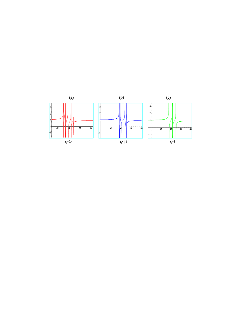
Figure 5: Dynamic permittivity of ideal films

A final number of resonating peaks is present, because $k_{z}$ component of exciton wave vector is discrete. Only for certain values of $k_{z}$ component for wave vector (with given values $k_{x}$ and $k_{y}$), resonating and radiation absorption may occur. Therefore, at least three and maximum five peaks occur - number is equal to number of permitted states along axis of translation symmetry breakage, in this case along z-axis. Due to the symmetry of model, distribution of peaks in complementary planes is the same: $n_{z}=0$ and $n_{z}=4$ (two boundary planes), as well as for $n_{z}=1$ and $n_{z}=3$ (first two inner planes). Only $n_{z}=2$ is different, since for the odd total number of atomic planes the middle plane has no complementary plane!

This result may be explained by experimental facts regarding resonating optical peaks in similar molecular layered nanostructures. In papers [23$-$25] this was evidenced in perylene chemical compounds (PTCDA, PTCS, PTFE and PBI) and explained by resonating effects at specific unoccupied levels. These effects are manifested by narrow optic absorption in close infra red band. In comparison with our results, which are concerning deeper infra red band in electromagnetic radiation, it may be concluded that these differences are effect of differences in crystalline (chemical and physical) structure as well as in the model (real and ideal) of samples investigated.

4 Conclusion

This paper describes original application of Paulian Green’s function method onto theoretical studies of optical properties of molecular crystals. Using Boson representation, microscopic (dispersion law and exciton state distribution) and macroscopic (dynamic permittivity) properties of these crystals may be successfully described.

Strictly following defined procedure, this paper shows that this method may be adapted and successfully applied to the study of dielectric properties in structures with disturbed spatial-translational symmetry, such as ultra thin films. Functioning of newly developed approach is illustrated through the problem of finding energy spectra and exciton states, as well as for determining relative permittivity of ideal monomolecular film.

In presence of two parallel boundaries in the system, energy spectrum is determined and possible exciton states were found. Important differences, comparing with unlimited crystalline structures, have been observed. Energy spectrum of excitons in monomolecular films is explicitly discrete, and the number of discrete levels is equal to the number of atomic planes (including boundary areas) along the axis of the spatial limitations of ultra thin film. In bulk sample, a single zone where excitons ”take” all possible energy values exists. All discrete levels are located within bulk boundaries, and the difference in zone width depends strictly (and inversely) on film thickness.

Comparing with bulk structures, where excitons may be found at any place with equal probability, in monomolecular film structures probability of finding exciton strongly depends on film thickness.

In exciton systems of monomolecular crystal bulk, where relative dynamic permittivity depends on frequency, continuous absorption zone exists in certain range of external radiation energy. In monomolecular film-structures resonating peaks exist with precisely determined energies, i.e. resonating frequencies. Number of these peaks depends on position of atomic plane (regarding boundary planes of the film) for which permittivity is being calculated: it decreases with the depth of ultra thin film.

Differences between properties of observed film and corresponding bulk structures drastically decrease as the thickness of film is higher. All this implies to the existence, and is a consequence, of the quantum size effects.

Method of Green’s differential functions, adapted on described manner should be applied further to the study of behavior and properties of more realistic quantum structures, for instance ultra thin films with perturbed boundary conditions.

Acknowledgements

Investigations whose results are presented in this paper were partially supported by the Serbian Ministry of Sciences (Grant No 141044) and by the Ministry of Sciences of the Republic of Srpska.

References

• [ 1] V. M. Agranovich and V. L. Ginzburg, Crystal-optic with Space
• [ 2] Ch. Kittel, Quantum Theory of Solids, Wiley & Sons, New York 1963.
• [ 3] G. Mahan, Many Particle Physics, Plenum Press, New York 1990.
• [ 4] M. G. Cottam and D.R.Tilley, Introduction to Surface and Superlattice Excitations, University Press, Cambridge 1989.
• [ 5] S. G. Davison and M. Steslicka, Basic Theory of Surface States, Clarendon Press, Oxford 1996.
• [ 6] V. M. Agranovich, K. Schmidt and K. Leo, Surface States in Molecular Chains with Strong Mixing of Frenkel and Charge-Transfer Excitons, Chem. Phys. Lett. 325 (2000) 308.
• [ 7] L. L. Chang and L. Esaki, Semiconductor Quantum Heterostructures, Phys. Today 45/10 (1992) 36.
• [ 8] I. Vragović, R. Scholz and M. Schreiber, Model Calculation of the Optical Properties of 3,4,9,10-Perylene-Tetracarboxylic-Dianhydride (PTCDA) Thin Films Europhys. Lett. 57 (2002) 288.
• [ 9] A. Langner, A. Hauschild, S. Fahrenholz and M. Sokolowski, Structural Properties of Tetracene Films on Ag(1 1 1) Investigated by SPA-LEED and TPD, Surface Science 574/2-3 (2005) 153.
• [10] W. J. Doherty III, A. G. Simmonds, S. B. Mendes, N. R. Armstrong and S. S. Saavedra, Molecular Ordering in Monolayers of an Alkyl-Substituted Perylene-Bisimide Dye by Attenuated Total Reflectance Ultraviolet-Visible Spectroscopy, Appl. Spectrosc. 9/10 (2005) 1248.
• [11] J. P. Šetrajčić, D. I. Ilić, B. Markoski, A. J. Šetrajčić, S. M. Vučenović, D. Lj. Mirjanić, B. Škipina, S. Pelemiš, Adapting and Application of the Green’s Functions Method onto Research of the Molecular Ultrathin Film Optical Properties, 15th Central European Workshop on Quantum Optics, Belgrade 2008.
• [12] I. D. Vragović, R. Scholz and J. P. Šetrajčić, Optical Properties of PTCDA Bulk Crystals and Ultrathin Films, Material Sience Forum 518 (2006) 41.
• [13] G. Rickayzen, Green’s Functions and Condensed Matter, Academic Press, London 1980.
• [14] E. N. Economou, Green’s Functions in Quantum Physics, Springer, Berlin 1949.
• [15] A. S. Davidov, Theory of Molecular Excitons, Nauka, Moskwa 1908. (in Russian)
• [16] M. C. Tringides, M. Jatochawski and E. Bauer, Quantum Size Effects in Metallic Nanostructures, Physics Today 60/4 (2007) 50.
• [17] I. Frenkel, On the Transformation of Light into Heat in Solids. I & II, Phys. Rev. 37 (1931) 17; 1276.
• [18] R. P. Djajić, D. Lj. Mirjanić, B. Nikin, J. P. Šetrajčić and B. S. Tošić, Stimulated Absorption in Ferroelectrics, J. Phys. C 20 (1987) 5585.
• [19] V. M. Agranovich, B. S. Toshich, Collective Properties of Frenkel Excitons, Zh. Eksp. Teor. Fiz. 53 (1967), 149 [Sov. Phys.-JETP 26 (1968), 104].
• [20] I. E. Dzyaloshinskii and L. P. Pitaevskii, Van der Waals Forces in an Inhomogeneous Dielectric, Zh. Eksp. Teor. Fiz 36 (1959) 1797 [Sov. Phys. JETP 9 (1959) 1282].
• [21] G. Arfken, Mathematical Methods for Physicists (3rd ed.), Academic Press, Orlando 1985.
• [22] T. J. Rivlin, Chebyshev Polynomials, Wiley, New York 1990.
• [23] A. B. Djurisic, T. Fritz and K. Leo, Modeling the Optical Constants of Organic Thin Films: Application to 3,4,9,10-Perylenetetracarboxylic Dianhydride (PTCDA), Opt. Commun. 183 (2000) 123.
• [24] R. Friedlen, M. P. de Jong, S. L. Sorensen, W. Osikowicz, S. Marciniak, G. Öwall, A. Lindgren and W. R. Salaneck, Resonant Auger Spectroscopy on Perylene, Porphyrine and Hexabenzocoronene Thin Films”, The 2nd Workshop on Advanced Spectroscopy of Organic Materials for Electronic Applications, Kanagawa 2003.
• [25] F. Würthner, C. Bauer, V. Stepanenko and S. Yagai, A Black Perylene Bisimide Super Gelator with an Unexpected J-Type Absorption Bank, Adv. Mater. 20 (2008) 1695.