MHD simulations of the magnetorotational instability in a shearing box with zero net flux: the case $Pm=4$

Abstract

Aims. This letter investigates the transport properties of MHD turbulence induced by the magnetorotational instability at large Reynolds numbers $Re$ when the magnetic Prandtl number $Pm$ is larger than unity.

Methods. Three MHD simulations of the magnetorotational instability (MRI) in the unstratified shearing box with zero net flux are presented. These simulations are performed with the code Zeus and consider the evolution of the rate of angular momentum transport as $Re$ is gradually increased from $3125$ to $12500$ while simultaneously keeping $Pm=4$. To ensure that the small scale features of the flow are well resolved, the resolution varies from $128$ cells per disk scaleheight to $512$ cells per scaleheight. The latter constitutes the highest resolution of an MRI turbulence simulation to date.

Results. The rate of angular momentum transport, measured using the $\alpha$ parameter, depends only very weakly on the Reynolds number: $\alpha$ is found to be about $7\times 10^{-3}$ with variations around this mean value bounded by $15\%$ in all simulations. There is no systematic evolution with $Re$. For the best resolved model, the kinetic energy power spectrum tentatively displays a power-law range with an exponent $-3/2$, while the magnetic energy is found to shift to smaller and smaller scales as the magnetic Reynolds number increases. A couple of different diagnostics both suggest a well–defined injection length of a fraction of a scaleheight.

Conclusions. The results presented in this letter are consistent with the MRI being able to transport angular momentum efficiently at large Reynolds numbers when $Pm=4$ in unstratified zero net flux shearing boxes.

1 Introduction

Angular momentum transport in accretion disks has been an outstanding issue in theoretical astrophysics for decades. To date the most likely mechanism appears to be MHD turbulence driven by the magnetorotational instability (MRI, Balbus & Hawley, 1991, 1998). Several numerical simulations have been performed to study its properties. The most popular approach is to work in the local approximation, using the shearing box model, as pioneered by Hawley et al. (1995), Hawley et al. (1996) or Brandenburg et al. (1995). These early simulations have shown that MRI–powered MHD turbulence is a robust mechanism that transports angular momentum outward. The rate of transport, measured by the famous $\alpha$ parameter (Shakura & Sunyaev, 1973) depends on the field geometry but is always positive, indicating outward flux of angular momentum. The results obtained in the 1990’s however obviously suffered from the limited computational resources available at that time. With no mean vertical magnetic field threading the shearing box (a field geometry referred to as the zero net flux case), Fromang & Papaloizou (2007) recently demonstrated with the code Zeus (Hawley & Stone, 1995) that it is indeed a problem: $\alpha$ decreases by a factor of two each time the resolution is doubled. This behavior has since been shown to be very robust as it has been confirmed by simulations performed with codes using different algorithms (Simon et al., 2009; Guan et al., 2009). This result, although it raised the concern that MRI–induced transport could vanish at infinite resolution, was interpreted as an indication that the small scale behavior of the flow is an important ingredient to determine the rate of MRI–induced angular momentum transport: small scale explicit dissipation coefficients, namely viscosity and resistivity, need to be included in the simulations. With such calculations Lesur & Longaretti (2007) showed that, for a nonzero vertical mean magnetic field, $\alpha$ rises with the magnetic Prandtl number $Pm$, the ratio of viscosity over resistivity. This result is actually very general: it is independent of the field geometry and was also found for a mean toroidal magnetic field (Simon & Hawley, 2009) and in the zero net flux case of interest here (Fromang et al., 2007). Recently Simon et al. (2009) measured the numerical dissipation properties of the code Athena (Gardiner & Stone, 2008; Stone et al., 2008). They found that an increase in resolution amounts to an increase of the numerical Reynolds numbers, while keeping the effective magnetic Prandtl number (i.e. the ratio between the numerical viscosity and the numerical resistivity) roughly constant and equal to about two. In light of these results a possible interpretation of the findings of Fromang & Papaloizou (2007) is that $\alpha$ is decreasing when the physical Reynolds number increases at fixed $Pm$. If unchecked, this decreasing $\alpha$ would mean that MRI–induced MHD turbulence is ineffective at transporting angular momentum without a mean flux, even in systems that have $Pm$ values higher than unity. Here, high resolution numerical simulations in which $Re$ and $Rm$ are simultaneously increased while keeping their ratio $Pm$ constant are used to examine if this is indeed the case.

2 Numerical setup

Model	Resolution	$Re$	$\alpha$
$Re3125$	$(128,192,128)$	3125	$7.9\times 10^{-3}\pm 4.5\times 10^{-4}$
$Re6250$	$(256,384,256)$	6250	$5.9\times 10^{-3}\pm 1.8\times 10^{-4}$
$Re12500$	$(512,768,512)$	12500	$8.4\times 10^{-3}\pm 3.8\times 10^{-4}$

Table 1: Properties of the simulations and time averaged value of $\alpha$. The errors on $\alpha$ are computed following Longaretti & Lesur (2010): the time history of $\alpha$ is divided in N bins of size $\tau$. $\tau$ is varied between $0.1$ and $8$ orbits. For each N, the standard deviation $\sigma_{N}$ is computed according to $\sigma_{N}=[\Sigma(\alpha_{i}-\alpha)/N]^{1/2}$, where $\alpha_{i}$ is the mean value in bin i. For large N, $\sigma_{N}$ scales like $N^{-1/2}$. The errors reported on $\alpha$ use that scaling to estimate $\sigma_{N}$ when $\tau=40$ orbits, the time duration over which the mean values of $\alpha$ are calculated.

In the simulations described below, the non–ideal MHD equations (i.e. including viscosity $\nu$ and resistivity $\eta$) are solved in the unstratified shearing box (Goldreich & Lynden-Bell, 1965) by the code Zeus (Hawley & Stone, 1995). The setup is identical to that used by Fromang et al. (2007): the shearing box rotates around the central point mass with angular velocity $\Omega$ (thus defining the orbital time $T_{orb}=2\pi/\Omega$), the equation of state is isothermal with the sound speed $c_{0}$, and the size of the box is fixed to $(L_{x},L_{y},L_{z})=(H,\pi H,H)$, where $H=c_{0}/\Omega$ is the disk scaleheight. As mentioned in the introduction, the magnetic flux threading the disk vanishes in all directions. Three simulations are presented here. They share the same value for the magnetic Prandtl number $Pm=\nu/\eta=4$. The Reynolds number $Re=c_{0}H/\nu$ is gradually increased from $Re=3125$ (hereafter labeled model $Re3125$) to $Re=6250$ (model $Re6250$) and finally $Re=12500$ (model $Re12500$). The resolution is increased at the same time as the Reynolds number to ensure that the smallest scale features of the flow are always resolved. Model $Re3125$ is identical to model $128Re3125Pm4$ of Fromang et al. (2007), for which different diagnostics have shown that $128$ cells per scaleheight are sufficient when using Zeus. Thus the resolutions $(N_{x},N_{y},N_{z})=(128,192,128)$, $(256,384,256)$ and $(512,768,512)$ are adopted respectively for model $Re3125$, $Re6250$ and $Re12500$. For model $Re12500$, it was found that early transients associated with the linear instability kept affecting the flow for long times, resulting in prohibitively long simulations. For the computational cost of that simulation to remain acceptable, the following procedure was used: model $Re3125$ was run from $t=0$ to $t=150$ orbits, starting from the initial state described above and identical to that used by Fromang et al. (2007). At $t=60$, the flow was interpolated on a grid twice finer. The dissipation coefficients were reduced by a factor of two and the model was restarted between $t=60$ and $t=150$ orbits. This constitutes model $Re6250$. This procedure was repeated at time $t=90$ orbits to produce model $Re12500$. The latter was run between $t=90$ and $t=135$ orbits. The properties of the three models are summarized in Table 1: the first column gives the label of the model, the second column reports its resolution $(N_{x},N_{y},N_{z})$ and the third the Reynolds number $Re$ for that run. All models share the same value $Pm=4$. Finally, the last column in Table 1 gives time–averaged values of $\alpha$ that are discussed in the subsections below.

3 Flow properties

In the three models flow features typical of unstratified shearing boxes simulations are recovered: weakly non–axisymmetric density waves propagate radially in the box (Heinemann & Papaloizou, 2009a, b) on top of smaller scales velocity and magnetic field turbulent fluctuations, the latter exhibiting a tangled structure typical of $Pm$ values higher than unity (Schekochihin et al., 2004). Below we concentrate on the transport properties of the turbulence, the shape of the kinetic and magnetic energy power spectra and the the two points correlation function.

3.1 Angular momentum transport

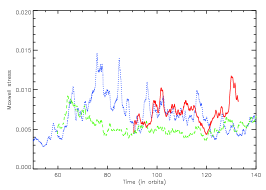
Figure 1: Time history of the Maxwell stress tensor for model $Re3125$ (blue dotted line), $Re6250$ (green dashed line) and $Re12500$ (red solid line). The three curves are consistent with the same time averaged value for $\alpha_{Max}$, independently of the Reynolds number.

The angular momentum transport properties of the turbulence in the three models are assessed by calculating the $\alpha$ parameter, the sum of the Reynolds stress tensor $\alpha_{Rey}$ and the Maxwell stress tensor $\alpha_{Max}$. All three coefficients are calculated as in Fromang & Papaloizou (2007). The time history of $\alpha_{Max}$ is shown in Fig. 1 for models $Re3125$, $Re6250$ and $Re12500$ respectively, using a dotted, a dashed and a solid line. The result is dramatically different from the results of Fromang & Papaloizou (2007) who found without explicit dissipation a monotonic decrease of $\alpha_{Max}$ as the resolution was increased. Here, no such systematic evolution is found as $Re$ goes up. Indeed $\alpha_{Max}$ appears to vary only very weakly with the Reynolds number. This is confirmed by the last column of Table 1 in which the values of $\alpha$, time–averaged between $90$ and $130$ orbits, are reported for the different models. The rate of angular momentum transport appears to be somewhat smaller in model $Re6250$ than in model $Re3125$ and $Re12500$. Nevertheless, the difference between the three simulations remains less than $25\%$. Taken together, the three measurements suggest that $\alpha$ is of the order of $7\times 10^{-3}$ and is fairly independent of the Reynolds number. At the very least, a systematic evolution of $\alpha$ with $Re$ is ruled out by the simulations.

3.2 Power spectrum

Figure 2: Top panel: kinetic (solid line) and magnetic (dashed line) energy power spectrum for model $Re12500$, time averaged over twenty snapshots between $t=90$ and $t=120$. The dotted line shows a power law line with index $-3/2$ for the purpose of comparison. Bottom panel: kinetic energy power spectra compensated by $1$ (dotted line), $3/2$ (solid line) and $5/3$ (dashed line). Both panels are suggestive of a $k^{-3/2}$ spectrum in the range $30<k<100$.

Figure 3: Top panel: plot of $E_{K}$ for model $Re3125$ (dotted line), $Re6250$ (dashed line) and $Re12500$ (solid line). The dotted line shows a power–law line with the index $-3/2$ for comparison. As $Re$ and $Rm$ increase, the kinetic energy display an increasing region well–fitted by a power law with the index $-3/2$, while the viscous cut–off region moves to higher $k$ values. Bottom panel: Same as the top panel, but for the quantity $kE_{M}$. On both panels the insets reproduce the results of Fromang & Papaloizou (2007) for model STD64 (dotted line), STD128 (dashed line) and STD256 (solid line).

The top panel of Fig. 2 shows the shell–averaged kinetic energy power spectrum $E_{K}$ (solid line) and magnetic energy power spectrum $E_{M}$ (dashed line) for model $Re12500$. The latter is rather flat over about a decade in wavenumber (from $k\sim 10$ to $k\sim 100$) and is larger than the kinetic energy over that range. By contrast, the former displays a clear power–law behavior for wavenumber $20<k<100$. For the purpose of comparison, the dotted line shows a pure power–law with the index $-3/2$ that nicely fits the solid line of the plot. By analogy with hydrodynamic turbulence it is tempting to associate the large scale end of the power–law part of the spectrum with an injection length $l_{inj}\sim 2\pi/k_{min}\sim 0.3H$. Similarly, the small scale end can be associated with the viscous cut–off length and is found to be $l_{visc}\sim 2\pi/k_{visc}\sim 0.06H$. This is about $32$ cells at that resolution and is thus well-resolved by the code. Furthermore, results obtained in the kinematic regime of incompressible and homogeneous MHD turbulence suggest that the resistive length $l_{res}\sim Pm^{-1/2}l_{visc}$ (Schekochihin et al., 2004). Thus, $l_{res}$ is of order $16$ cells and also well resolved, which shows that numerical dissipation is most likely negligible in this simulation. Given the still limited resolution of model $Re12500$, the reliability of the power–law exponent mentioned above can however be questioned: for that purpose, the bottom panel of Fig. 2 displays three compensated spectra of $E_{K}$, $kE_{K}$ (dotted line), $k^{3/2}E_{K}$ (solid line) and $k^{5/3}E_{K}$ (dashed line) respectively. First, the figure illustrates the difficulty of a reliable determination of the exponent. Indeed, the power–law extends over less than a decade in wavenumber. Nevertheless, the dashed line, which unambiguously rises over the interval of $10<k<100$, excludes a $k^{-5/3}$ spectrum and rather suggests an exponent larger than $-5/3$. The dotted line on the other hand suggests $-1$ as an upper limit. Finally, the solid line suggests $k^{-3/2}$ as a tentative fit for the power–law range of the spectrum ($30<k<100$). Finally, Fig. 3 (top panel) compares the shape of $E_{K}$ in model $Re3125$ (dotted line), $Re6250$ (dashed line) and $Re12500$ (solid line). For all models, the kinetic energy power spectrum peaks at $k\sim 10$–$20$. For larger wavenumbers, the $k^{-3/2}$ power–law becomes more and more apparent as the Reynolds number increases. The bottom panel of Fig. 3 plots the quantity $kE_{M}$ for the three simulations. The peak of each curve thus provides an estimate of the scale at which magnetic energy is located. It is found to lie at $k_{peak}\sim 30$–$40$, $50$–$60$ and $70$–$80$ respectively when $Re=3125$, $6250$ and $12500$. In other words, the scale at which most of the magnetic energy is located moves toward smaller and smaller scales as $Rm$ is increased. This is different from the results reported by Haugen et al. (2003), but not unexpected given existing theories of small scale dynamos with large $Pm$ (Schekochihin et al., 2002a, b). On both panels, the small insets plot the spectra obtained by Fromang & Papaloizou (2007) without explicit dissipation. Aside from the decrease of their amplitude with resolution, the most noticable differences with the results presented here are twofold: first, the kinetic energy power–spectra appear flatter at intermediate wavenumbers. In addition, there is more energy (both kinetic and magnetic) at the smallest scales of the box.

3.3 Correlation length

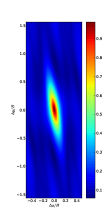
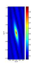
Figure 4: Structure of the correlation function $\xi_{v}$ in the $(\Delta_{x},\Delta_{y})$ plane for model $Re3125$ (left panel), $Re6250$ (middle panel) and $Re12500$ (right panel). Its structure is only weakly dependent on the Reynolds number, suggesting a well–defined injection length.

The shape of the kinetic energy power–spectrum described above suggests an injection length $l_{inj}$ that appears to be independent of $Re$ for the range of the Reynolds numbers investigated here. However, the shell average involved in its derivation washes out all information about the anisotropy of the turbulence. This can be investigated using the two–points–correlation function (Guan et al., 2009; Davis et al., 2010):

$$\xi_{v}(\mbox{\boldmath{$\Delta x$}})=\textrm{$<$}\Sigma_{i}\delta v_{i}(\mbox{\boldmath{$x$}})\delta v_{i}(\mbox{\boldmath{$x$}}+\mbox{\boldmath{$\Delta x$}})\textrm{$>$}/\textrm{$<$}\Sigma_{i}\delta v_{i}^{2}\textrm{$>$}\,.$$ (1)

Here $<$.$>$ stands for a volume average, $\delta v_{i}(\mbox{\boldmath{$x$}})$ corresponds to the velocity fluctuations in the direction i and the sum is over spatial coordinates. Isocontours of $\xi_{v}$ in the plane $\Delta z=0$ are shown in Fig. 4. From left to right, the different panels correspond to models $Re3125$, $Re6250$ and $Re12500$ respectively. As found by Guan et al. (2009) and Davis et al. (2010), $\xi_{v}$ has an ellipsoidal shape for all models. The tilt angle $\theta_{v}$ of the major axis is $\theta_{v}$$\sim$$8$ degrees, which agrees with the results of Guan et al. (2009). Following the procedure outlined by these authors (i.e. by fitting the shape of the correlation function in a given direction by an exponential), the correlation lengths along the major, minor and vertical axis of the ellipsoid are found to be $(\lambda_{min},\lambda_{max},\lambda_{z})=(0.08,0.45,0.08)H$, independently of the Reynolds number. This suggests once more that the injection length of the turbulence is only weakly dependent on the Reynolds number. At the same time, the small difference between $\lambda_{min}$ or $\lambda_{z}$ and $l_{visc}$ as quoted in section 3.2 is a warning that the injection range and the dissipative range might overlap in these simulations.

4 Conclusion

Here zero net flux high resolution numerical simulations of MRI–driven MHD turbulence are used to demonstrate this result: when $Pm$$=$$4$, the dependence of $\alpha$ on the Reynolds number is very weak. In all models, $\alpha\sim 7\times 10^{-3}$ to within about $15\%$. This result unambiguously shows that the decrease of $\alpha$ with resolution reported by Fromang & Papaloizou (2007) is a numerical artifact that contains no physical information about the nature of the MHD turbulence in accretion disks. Quite differently, the present simulations are consistent with a nonzero value of $\alpha$ at infinite Reynolds numbers for a magnetic Prandtl number higher than unity. Note that this weak dependence of $\alpha$ with $Re$ for $Pm>1$ is also suggested by the data recently reported by Simon & Hawley (2009) and Longaretti & Lesur (2010) respectively for a mean azimuthal and vertical magnetic field.

In addition, a number of statistical properties of the turbulence are reported. The kinetic energy power spectrum of the turbulence and the two–points–correlation function of the velocity both suggest a well–defined injection length $l_{inj}$ of a few tens of a scaleheight. For the range of the Reynolds numbers $Re$ that can be probed with current resources, $l_{inj}$ seems to be independent of $Re$. At the highest resolution achieved here, the kinetic energy power spectrum displays a power–law scaling over almost a decade in wavenumber. However, given the limited extent of the power–law range, the precise exponent of this power–law cannot be accurately determined: an exponent of $-3/2$ appears to be consistent with the data, while a $-5/3$ exponent seems too steep. Nevertheless, as suggested in Sect. 3.3, the separation between the forcing and the dissipative scales might still be marginal. This is why a detailed comparison of these exponents with existing MHD turbulence theories (Iroshnikov, 1963; Kraichnan, 1965; Goldreich & Sridhar, 1995) is probably premature at this stage. Higher resolution simulations are definitively needed. Finally, the shape of the magnetic energy power spectrum shows that magnetic energy is mostly located at small scales and shifts to smaller and smaller scales as $Rm$ increases, as expected from small scale dynamo theory (Schekochihin et al., 2002a). This is consistent with the scenario postulated by Rincon et al. (2008) of a large scale MRI forcing that generates and coexists with a small scale dynamo.

References

- Balbus & Hawley (1991) Balbus, S. & Hawley, J. 1991, ApJ, 376, 214
- Balbus & Hawley (1998) Balbus, S. & Hawley, J. 1998, Rev.Mod.Phys., 70, 1
- Brandenburg et al. (1995) Brandenburg, A., Nordlund, A., Stein, R. F., & Torkelsson, U. 1995, ApJ, 446, 741
- Davis et al. (2010) Davis, S. W., Stone, J. M., & Pessah, M. E. 2010, ApJ, 713, 52
- Fromang & Papaloizou (2007) Fromang, S. & Papaloizou, J. 2007, A&A, 476, 1113
- Fromang et al. (2007) Fromang, S., Papaloizou, J., Lesur, G., & Heinemann, T. 2007, A&A, 476, 1123
- Gardiner & Stone (2008) Gardiner, T. A. & Stone, J. M. 2008, Journal of Computational Physics, 227, 4123
- Goldreich & Lynden-Bell (1965) Goldreich, P. & Lynden-Bell, D. 1965, MNRAS, 130, 125
- Goldreich & Sridhar (1995) Goldreich, P. & Sridhar, S. 1995, ApJ, 438, 763
- Guan et al. (2009) Guan, X., Gammie, C. F., Simon, J. B., & Johnson, B. M. 2009, ApJ, 694, 1010
- Haugen et al. (2003) Haugen, N. E. L., Brandenburg, A., & Dobler, W. 2003, ApJ, 597, L141
- Hawley & Stone (1995) Hawley, J. & Stone, J. 1995, Comput. Phys. Commun., 89, 127
- Hawley et al. (1995) Hawley, J. F., Gammie, C. F., & Balbus, S. A. 1995, ApJ, 440, 742
- Hawley et al. (1996) Hawley, J. F., Gammie, C. F., & Balbus, S. A. 1996, ApJ, 464, 690
- Heinemann & Papaloizou (2009a) Heinemann, T. & Papaloizou, J. C. B. 2009a, MNRAS, 397, 52
- Heinemann & Papaloizou (2009b) Heinemann, T. & Papaloizou, J. C. B. 2009b, MNRAS, 397, 64
- Iroshnikov (1963) Iroshnikov, P. S. 1963, AZh, 40, 742
- Kraichnan (1965) Kraichnan, R. H. 1965, Physics of Fluids, 8, 1385
- Lesur & Longaretti (2007) Lesur, G. & Longaretti, P.-Y. 2007, MNRAS, 378, 1471
- Longaretti & Lesur (2010) Longaretti, P. & Lesur, G. 2010, A&A, accepted
- Rincon et al. (2008) Rincon, F., Ogilvie, G. I., Proctor, M. R. E., & Cossu, C. 2008, Astronomische Nachrichten, 329, 750
- Schekochihin et al. (2002a) Schekochihin, A. A., Boldyrev, S. A., & Kulsrud, R. M. 2002a, ApJ, 567, 828
- Schekochihin et al. (2004) Schekochihin, A. A., Cowley, S. C., Taylor, S. F., Maron, J. L., & McWilliams, J. C. 2004, ApJ, 612, 276
- Schekochihin et al. (2002b) Schekochihin, A. A., Maron, J. L., Cowley, S. C., & McWilliams, J. C. 2002b, ApJ, 576, 806
- Shakura & Sunyaev (1973) Shakura, N. I. & Sunyaev, R. A. 1973, A&A, 24, 337
- Simon & Hawley (2009) Simon, J. B. & Hawley, J. F. 2009, ApJ, 707, 833
- Simon et al. (2009) Simon, J. B., Hawley, J. F., & Beckwith, K. 2009, ApJ, 690, 974
- Stone et al. (2008) Stone, J. M., Gardiner, T. A., Teuben, P., Hawley, J. F., & Simon, J. B. 2008, ApJS, 178, 137