An Updated Numerical Analysis of eV Seesaw with Four Generations

Abstract

We consider the so-called “eV seesaw” scenario, with right-handed Majorana mass $M_{R}$ at eV order, extended to four lepton generations. The fourth generation gives a heavy pseudo-Dirac neutral lepton, which largely decouples from other generations and is relatively stable. The framework naturally gives 3 active and 3 sterile neutrinos. We update a previous numerical analysis of a 3+3 study of the LSND anomaly, taking into account the more recent results from the MiniBooNE experiment. In particular, we study the implications for the third mixing angle $\mathrm{sin}^{2}\theta_{13}$, as well as CP violation. We find that current data do not seriously constrain more than one sterile neutrinos.

I Introduction

Neutrino data hint at the possibility of something beyond three massive, mostly active neutrinos. The LSND result of $P(\bar{\nu}_{\mu}\rightarrow\bar{\nu}_{e})=0.264\%$ Lsnd1 can be explained if there exist one sterile neutrino, with $\Delta m^{2}\sim 1\ \rm{eV}^{2}$ with respect to other neutrinos. This lead to the so-called “eV seesaw” scenario Gouvea , where the right-handed neutrino Majorana scale $M_{R}$ is taken to be of eV order. In 2006, the eV seesaw scenario was extended to four lepton generations Hou1 . The fourth generation gives rise to a heavy pseudo-Dirac neutral lepton, which largely decouples from the other generations, and is relatively stable. The framework gives naturally 3 active and 3 sterile neutrinos (3+3).

Motivated by the interpretation of the $\bar{\nu}_{e}$ excess observed by LSND in terms of $\bar{\nu}_{\mu}\rightarrow\bar{\nu}_{e}$ antineutrino oscillations, the MiniBooNE (MB) experiment was constructed. In 2007, the MiniBooNE collaboration presented Miniboone1 their first results of a search for $\nu_{\mu}\rightarrow\nu_{e}$ neutrino oscillations, which did not support the LSND excess, but some excess at low energy was not fully understood. Taking this result into account, Maltoni and Schwetz Maltoni1 found that the 3+2 scheme can fit both LSND $\bar{\nu}_{\mu}\rightarrow\bar{\nu}_{e}$ data and MB $\nu_{\mu}\rightarrow\nu_{e}$ data, and at the same time account for the excess of low energy events in MB data. More recently, the MiniBooNE collaboration reported their latest data, updating neutrino results Miniboone2 (including the low energy region), as well as the first antineutrino results Miniboone3 , and first results from the off-axis NuMI beam observed in the MiniBooNE detector Adamson . Motivated by these new results, the authors of Ref. Karagiorgi re-examined the 3+1 and 3+2 global fits to the short-baseline (SBL) data. They found that the 3+2 oscillation hypothesis provides only a marginally better description of all SBL data over the 3+1 oscillation hypothesis. In addition, a 3+1 fit to all antineutrino SBL data (MiniBooNE($\bar{\nu}$), LSND, KARMEN KARMEN , Bugey Bugey , and CHOOZ CHOOZ ) can yield $86\%$ $\chi^{2}$-probability and high compatibility.

In this paper we update the previous numerical analysis of the 3+3 study of the LSND anomaly, taking into account MB data. In particular, we consider the implications for the third mixing angle, and CP violation. The outline is as follows. In Sec. II we update the previous numerical solutions by inputting the latest neutrino oscillation parameters from global data. In Sec. III we add the CP violation phases to the leptonic mixing matrix and investigate the effect of phase factors, and give a short summary in Sec. IV.

II UPDATED NUMERICAL ANALYSIS

II.1 Updated Fit

In Ref. Maltoni1 , Maltoni and Schwetz discussed different types of oscillation frameworks that include one or more sterile neutrinos at the eV scale, by considering the global short-baseline (SBL) experiments data which included the MiniBooNE first result Miniboone1 . The analysis built on an earlier study which showed that MiniBooNE (2007), LSND, and the null appearance experiments (KARMEN and NOMAD NOMAD ) are compatible under a 3+2 sterile neutrino oscillation scenario with large CP violation. Recently, in light of recently published results from the MiniBooNE experiment Miniboone2 ; Miniboone3 ; Adamson , Karagiorgi et al. Karagiorgi re-examined sterile neutrino oscillation models. They found that, with the addition of the new MiniBooNE data sets, a 3+2 oscillation hypothesis provides only a marginally better description of all short-baseline data over a 3+1 oscillation hypothesis. On the other hand, fits to antineutrino-only data sets, including appearance and disappearance experiments, are found significantly more compatible, even within a 3+1 oscillation scenario. We shall therefore use the best-fit values for mass splittings and mixing angles obtained from 3+1 fits to all antineutrino SBL data in Ref. Karagiorgi , and the corresponding projected value of the LSND probability $P(\bar{\nu}_{\mu}\rightarrow\bar{\nu}_{e})=0.2334\%$ Thomas .

Table 1: Best fit values, $1\sigma$ and $3\sigma$ intervals for three-flavor neutrino oscillation parameters taken from Ref. GonzalezGarcia:2010er .

	BEST FIT	$1\sigma$	$3\sigma$
$\Delta m_{21}^{2}\,(10^{-5}\;{\rm eV}^{2})$	$7.59$	$7.39-7.79$	$6.90-8.20$
$\Delta m_{31}^{2}\,(10^{-3}\;{\rm eV}^{2})$	$+2.47$	$+(2.35-2.59)$	$+(2.10-2.84)$
	$-2.36$	$-(2.29-2.43)$	$-(2.00-2.72)$
$\sin^{2}{\theta_{12}}$	$0.32$	$0.30-0.34$	$0.28-0.37$
$\sin^{2}{\theta_{23}}$	$0.46$	$0.41-0.53$	$0.34-0.65$
$\sin^{2}{\theta_{13}}$	$0.014$	$0.005-0.025$	$\leq 0.049$

Table 2: Seven inputs taken from Ref. GonzalezGarcia:2010er ; Thomas ; Karagiorgi and the best fit values from the minimization process.

	INPUT	2010
$P(\bar{\nu}_{\mu}\rightarrow\bar{\nu}_{e})(\%)$	$0.2334$	$0.2090$
$\Delta m_{21}^{2}\,(10^{-5}\;{\rm eV}^{2})$	$7.59$	$7.59$
$\Delta m_{31}^{2}\,(10^{-3}\;{\rm eV}^{2})$	$2.5$	$2.5$
$\Delta m_{41}^{2}\,({\rm eV}^{2})$	$1$	$1$
$\sin^{2}{\theta_{12}}$	$0.32$	$0.32$
$\sin^{2}{\theta_{23}}$	$0.46$	$0.46$
$\sin^{2}{\theta_{13}}$	$0.014$	$0.014$

We shall not recount the effective 3+3 formalism that arises from the eV seesaw model with 4 generations, which we refer to Ref. Hou1 . Our purpose is to assess how the numerics and conclusions are affected by the new data. To perform our numerical analysis of a 3+3 picture, we build the $\chi^{2}$ by using the three-flavor neutrino oscillation parameters $\Delta m_{ji}^{2}$ and $\sin^{2}{\theta_{ij}}$ taken from Ref. GonzalezGarcia:2010er , which are the results of the global combined analysis done in the framework of the AGSS09 solar fluxes Serenelli:2009yc and the modified Ga capture cross-section in Ref. Abdurashitov:2009tn . These are given explicitly in Table I. We also include the projected value of $P(\bar{\nu}_{\mu}\rightarrow\bar{\nu}_{e})=0.2334\%$ Thomas , and require $\Delta m^{2}_{41}\sim 1\,{\rm eV}^{2}$ as in the previous analysis. The seven inputs are listed in the second column in Table II.

As there are many more parameters, one cannot make a proper fit, so we just seek to minimize the $\chi^{2}$ by varying the model parameters. In this way, we obtain the values for the twelve parameters $r_{ij}$, $\epsilon_{i}$ and $s_{i}$ (see Ref. Hou1 for definition) of the model at the best fit point, which are given in Table III. These would be further illustrated below. We then use these parameter values to get the expectation values for the seven observables, which are listed in the third column in Table II. For comparison, the results from the 2006 study Hou1 is given in Table IV.

Table 3: Parameter values of the best fit point, where the parameters are defined in Ref. Hou1 .

Parameter	$\epsilon_{1}$	$\epsilon_{2}$	$\epsilon_{3}$	$s_{1}$	$s_{2}$	$s_{3}$
BEST FIT	$0.049$	$0.018$	$0.039$	$0.102$	$0.9999$	$-0.72$
Parameter	$r_{11}$	$r_{12}$	$r_{13}$	$r_{22}$	$r_{23}$	$r_{33}$
BEST FIT	$1.263$	$0.852$	$1.042$	$1.187$	$0.742$	$1.223$

Table 4: Inputs Lsnd1 ; Maltoni2 and the best fit values from in 2006 Hou1 , to be compared with Table II.

	INPUT	2006
$P(\bar{\nu}_{\mu}\rightarrow\bar{\nu}_{e})(\%)$	$0.264$	$0.15$
$\Delta m_{21}^{2}\,(10^{-5}\;{\rm eV}^{2})$	$8.1$	$8.1$
$\Delta m_{31}^{2}\,(10^{-3}\;{\rm eV}^{2})$	$2.2$	$2.3$
$\Delta m_{41}^{2}\,({\rm eV}^{2})$	$1$	$1$
$\sin^{2}{\theta_{12}}$	$0.30$	$0.30$
$\sin^{2}{\theta_{23}}$	$0.50$	$0.52$
$\sin^{2}{\theta_{13}}$	$0.0$	$0.0018$

Comparing these two tables, we can see that the difference between best fit values and expected (input) values of $P(\bar{\nu}_{\mu}\rightarrow\bar{\nu}_{e})$ in Table II is smaller than the difference in Table IV, not just for $P(\bar{\nu}_{\mu}\rightarrow\bar{\nu}_{e})$, but also for, e.g. $\sin^{2}{\theta_{23}}$. Comparing the $\chi^{2}$, we find

$$\chi^{2}_{\rm min,2006}-\chi^{2}_{\rm min,2010}=1.83,$$ (1)

where $\chi^{2}_{\rm min,2006}$ and $\chi^{2}_{\rm min,2010}$ are the $\chi^{2}$ minima for best fit values in 2006 and 2010. One could say that the agreement between the scenario of eV seesaw with four generations and the experimental data has improved.

II.2 In Search of Sizable $\sin^{2}{\theta_{13}}$

The plausible value for $\sin^{2}{\theta_{13}}$, the target of Daya Bay and T2K experimemnts, is of great interest. To discuss this, as in Ref. Hou1 , we restrict the $\chi^{2}$ to the four inputs of $\sin^{2}{\theta_{ij}}$ and $P(\bar{\nu}_{\mu}\rightarrow\bar{\nu}_{e})$. With $\epsilon_{i}$ and $r_{ij}$ given as in Table III, we first fix $s_{1}=0.1$, the best fit value, and perform a $\chi^{2}$ fit vs $s_{2}$ and $s_{3}$, then iterate with fixing $s_{2}=0.9999$ ($s_{3}=-0.72$) and minimize $\chi^{2}$ vs $s_{1}$ and $s_{3}$ ($s_{1}$ and $s_{2}$). We find for both cases of fixing $s_{1}$ or $s_{3}$ to the best fit values, $\sin^{2}{\theta_{23}}$ is quite strongly dependent on $s_{2}$, and the value around 0.9999 is preferred. We thus illustrate with $s_{2}$ held fixed to this value.

Fig. 1: Contour-plot of $\chi^{2}$ vs the mixing angles $s_{1}$ and $s_{3}$, with $\epsilon_{i}$ and $r_{ij}$ as in Table IV, and $s_{2}=0.9999$ held fixed. The regions in different shades are only indicative, and should not be interpreted as the $1\sigma$, $2\sigma$ and $3\sigma$ regions, as the rest of the parameters are fixed at the best fit values.

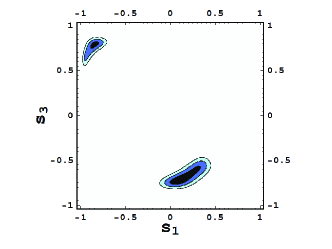
In Fig. 1 we show the $\chi^{2}$ contour plot vs $s_{1},s_{3}$. The three different shaded regions should not be interpreted as the $1\sigma$, $2\sigma$ and $3\sigma$ regions, since we have fixed the rest of the parameters to the best fit values. But they do give an indication of variations around the best fit region under the above assumptions. The gross features are not too different from the 2006 study. For the lower right solution, $s_{1}$ has moved closer to zero, and the strength of $s_{3}$ has also weakened a little. For the upper left solution, $s_{3}$ is little changed, but $s_{1}$ has strengthened considerably, moving the solution more into the corner.

Fig. 2: $P(\bar{\nu}_{\mu}\rightarrow\bar{\nu}_{e})$, $\sin^{2}{\theta_{12}}$, $\sin^{2}{\theta_{23}}$ and $\sin^{2}{\theta_{13}}$ vs $s_{1}$ and $s_{3}$, corresponding to the lower right solution in Fig. 1, with $\epsilon_{i}$ and $r_{ij}$ fixed as in Table III, and $s_{2}$ fixed at 0.9999.

Fig. 3: Same as Fig. 2, but corresponding to the upper left solution in Fig. 1.

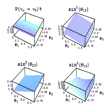
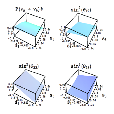
We plot in Fig. 2 the four quantities $P(\bar{\nu}_{\mu}\rightarrow\bar{\nu}_{e})$, $\sin^{2}{\theta_{12}}$, $\sin^{2}{\theta_{23}}$ and $\sin^{2}{\theta_{13}}$ vs $s_{1}$ and $s_{3}$, for the solution on the lower right of Fig. 1. The same is plotted in Fig. 3 for the upper left solution. Again, $\epsilon_{i}$ and $r_{ij}$ are fixed as in Table III, and $s_{2}$ is held fixed at 0.9999. The dependence on $s_{1}$–$s_{3}$, or shape, for $P(\bar{\nu}_{\mu}\rightarrow\bar{\nu}_{e})$ differs somewhat from the 2006 case, with the lower right solution now allowing larger values. We see that $P(\bar{\nu}_{\mu}\rightarrow\bar{\nu}_{e})$ can reach $0.2\%$ and $\sin^{2}{\theta_{12}}$ is well within range, and likewise for $\sin^{2}{\theta_{23}}$. However, to push $\sin^{2}{\theta_{13}}$ beyond 0.025, $\sin^{2}{\theta_{23}}$ would start to wander away from maximal mixing of 0.5, and values at $\sim 0.4$ or 0.6 has to be tolerated. The situation is not much changed from 2006, but we note that the slightly more promising situation for $\sin^{2}{\theta_{13}}$ can be traced to the more positive input value in Table II, which now does include SBL data.

II.3 Neutrino Mass Hierarchy

The sign of $\Delta m_{31}^{2}$ is undetermined by present data (e.g. MINOS experiment). That is to say, the neutrino mass hierarchy is not known at this time. We use eV seesaw with four generations scenario to see if we can gain any access to the neutrino mass hierarchy. For normal mass hierarchy, the sign of $\Delta m_{31}^{2}$ is positive and the best fit value is $2.47\times 10^{-3}\;{\rm eV}^{2}$, and the numerical analysis has been performed in the previous section. For inverted mass hierarchy, the sign of $\Delta m_{31}^{2}$ is negative with best fit value $-2.36\times 10^{-3}\;{\rm eV}^{2}$. To perform the numerical analysis for inverted mass hierarchy, we use the best fit values given as in Table III but only replacing that of $\Delta m_{31}^{2}$ by $-2.36\times 10^{-3}\;{\rm eV}^{2}$ to work out $\chi^{2}$ minimum. Comparing with the $\chi^{2}$ minimum for normal mass hierarchy, we find

$$\chi^{2}_{\rm min,inverted}-\chi^{2}_{\rm min,normal}=1.74,$$ (2)

in obvious notation. It seems that the agreement of eV seesaw with four generations scenario with normal mass hierarchy is slightly better than the agreement with inverted mass hierarchy. We caution that our study is not a true fit, as there are too many model parameters.

III CP VIOLATION

So far, we have not considered CP violation effect, and all phases in the leptonic mixing matrix were set to zero for simplicity, just as in the previous paper Hou1 . As defined in Ref. Hou1 , $U^{\prime}$ and $U^{\prime\prime}$ are the rotation matrices which diagonalize the neutrino and charged-lepton mass matrices, respectively, and the full leptonic mixing matrix is $U=U^{\prime\prime}U^{\prime}$. Although introducing CP violation phase to the leptonic mixing matrix adds further to the already many parameters, there is some motivation to study CP violation effect, in part because there are both neutrino and antineutrino oscillation data, and they appear to be somewhat different. We shall therefore give two examples for illustration.

III.1 Refit with CP Violation Phase

As charged lepton masses are generated by the Higgs mechanism, similar to quark masses, we take the left sector rotation matrix $U^{\prime\prime}$ to be the usual form

$${\scriptsize U^{\prime\prime}=\left(\begin{array}[]{cccccc}c_{1}c_{3}&s_{1}c_{3}&s_{3}e^{-i\delta}&0&0&0\\ -s_{1}c_{2}-c_{1}s_{2}s_{3}e^{i\delta}&c_{1}c_{2}-s_{1}s_{2}s_{3}e^{i\delta}&s_{2}c_{3}&0&0&0\\ s_{1}s_{2}-c_{1}c_{2}s_{3}e^{i\delta}&-c_{1}s_{2}-s_{1}c_{2}s_{3}e^{i\delta}&c_{2}c_{3}&0&0&0\\ 0&0&0&1&0&0\\ 0&0&0&0&1&0\\ 0&0&0&0&0&1\\ \end{array}\right)},$$ (3)

where $\delta$ is the CP violation phase and placed in the $13$ element of $U^{\prime\prime}$. Because of the presence of $\delta$, the formulas for $P(\bar{\nu}_{\mu}\rightarrow\bar{\nu}_{e})$ would no longer be equal to that of $P(\nu_{\mu}\rightarrow\nu_{e})$. We use this new $U^{\prime\prime}$ matrix with CP violation phase $\delta$, and the best fit values given as in Table II for inputs, and redo our numerical analysis. After minimization, we get the new $\chi^{2}$ minimum, i.e. $\chi^{2}_{\rm min,CP}$. We find that introducing CP phase $\delta$ leads to the relative improvement of the fit of

$$\chi^{2}_{\rm min,2010}-\chi^{2}_{\rm min,CP}=0.004,$$ (4)

which is negligible. The quality of the global fit does not improve at all by introducing CP violation phase. But this is somewhat trivial, since Table II tacitly assumes CP conservation.

Table 5: Same as Table II, but adding a null $\nu_{\mu}\rightarrow\nu_{e}$ oscillation probability as input, together with the expectation values from the minimization process.

	INPUT
$P(\bar{\nu}_{\mu}\rightarrow\bar{\nu}_{e})(\%)$	$0.2334$	$0.1423$
$P(\nu_{\mu}\rightarrow\nu_{e})(\%)$	$0$	$0.048$
$\Delta m_{21}^{2}\,(10^{-5}\;{\rm eV}^{2})$	$7.59$	$7.59$
$\Delta m_{31}^{2}\,(10^{-3}\;{\rm eV}^{2})$	$2.5$	$2.5$
$\Delta m_{41}^{2}\,({\rm eV}^{2})$	$1$	$1$
$\sin^{2}{\theta_{12}}$	$0.32$	$0.32$
$\sin^{2}{\theta_{23}}$	$0.46$	$0.43$
$\sin^{2}{\theta_{13}}$	$0.014$	$0.017$

III.2 An Extreme Example of CP Violation

The updated MiniBooNE $\nu_{\mu}\rightarrow\nu_{e}$ result indicates an excess of $\nu_{e}$ events at low energy, but no $\nu_{\mu}\rightarrow\nu_{e}$ oscillations at the $L/E\sim 1\,{\rm m/MeV}$ of the LSND excess, which is for antineutrinos. Furthermore, neither NUMI Adamson nor NOMAD NOMAD found evidence for $\nu_{\mu}\rightarrow\nu_{e}$ oscillations. Thus, we consider $P(\nu_{\mu}\rightarrow\nu_{e})=0\%$ at $L/E=1\,{\rm m/MeV}$ as a new additional input, to illustrate an extreme situation where there is a striking difference between the behavior of $\nu_{\mu}\rightarrow\nu_{e}$ and $\bar{\nu}_{\mu}\rightarrow\bar{\nu}_{e}$ oscillations. We stress that this is only an illustration, since neither the LSND effect for $\bar{\nu}_{\mu}\rightarrow\bar{\nu}_{e}$ oscillations, nor the absence of $\nu_{\mu}\rightarrow\nu_{e}$, are firmly established. Furthermore, we clearly have too many parameters, hence we are just performing $\chi^{2}$ illustrations, not a fit.

The new ad hoc input, together with the 7 inputs of Table II, are now listed in Table V, with which we build the new $\chi^{2}$ in the framework with CP violation. After minimizing the $\chi^{2}$, we use the thirteen parameter values of the best fit point to get the the expectation values for the eight observables, which are listed in the third column in Table V. There is now a slight tension in $\sin^{2}\theta_{23}$ (though allowed), while neither the antineutrino, nor the neutrino oscillation probabilities can reach the input values, but this may be reasonable. The best fit value of CP violation phase $\delta$ is $0.37\pi$, or of order $66^{\circ}$, which is of course rather large. Note also that the $\sin^{2}{\theta_{13}}$ value is now larger than in Table II, which is again reasonable, since a finite $\sin^{2}{\theta_{13}}$ is a prerequisite for CP violation. This illustrates the efficacy of the Daya Bay and T2K experiments, as well as a future CPV program.

IV Summary

We have updated the numerics of a 3+3 active/sterile neutrino picture, which arises naturally from a four lepton generation model with eV seesaw, i.e. with right-handed Majorana mass scale $M_{R}$ at eV order. The major new data are the MiniBooNE results of the past few years, which do not confirm the LSND $\bar{\nu}_{\mu}\rightarrow\bar{\nu}_{e}$ result. Since the 3+3 model has too many parameters, while data is more or less consistent with a 3+1 picture, we take global fit results using the latter framework as input, and use a $\chi^{2}$ minimization to find the best values for neutrino mass differences, mixing angles, and $\bar{\nu}_{\mu}\rightarrow\bar{\nu}_{e}$ probability. Not unexpectedly, the consistency of the 3+3 picture with current data improves over the consistency with data in 2006. We continue to find it difficult for $\sin^{2}{\theta_{13}}$ to be larger than 2.5%, while finding a slightly better $\chi^{2}$ for normal mass hierarchy over the inverted mass hierarchy. These, however, could be artefacts of not being able to do a real fit.

If one continues to take the LSND $\bar{\nu}_{\mu}\rightarrow\bar{\nu}_{e}$ result seriously (which provides the eV scale), together with the consensus of null results for $\nu_{\mu}\rightarrow\nu_{e}$ oscillations, we have put in the CP violation phase in the charged lepton mixing matrix, and illustrated the possibility of CP violation. The world of large CP violation effect in $\bar{\nu}_{\mu}\rightarrow\bar{\nu}_{e}$ vs $\nu_{\mu}\rightarrow\nu_{e}$ oscillations, with large CPV phase and finite $\sin^{2}{\theta_{13}}$, could be a striking one.

Note Added. Our Table I uses version 2 of Ref. GonzalezGarcia:2010er , which is the published one. Subsequently, these authors have posted version 3 on the arXiv, which includes new results on $\nu_{e}$ appearance from MINOS, which leads to a smaller $\sin^{2}{\theta_{13}}$ (best fit at 0.008). However, we have discussed how things will be for a lower $\sin^{2}{\theta_{13}}$, so we leave the paper as is.

Acknowledgement.  We thank T. Schwetz and G. Karagiorgi for useful communications. The work of WSH is supported in part by NSC97-2112-M-002-004-MY3 and NTU-98R0066. The work of FFL is supported by NSC98-2811-M-002-102.

References

- (1) A. Aguilar et al. (LSND Collaboration), Phys. Rev. D 64, 112007 (2001).
- (2) A. de Gouvêa, Phys. Rev. D 72, 033005 (2005).
- (3) W.-S. Hou and A. Soddu, Phys. Lett. B 638, 229 (2006).
- (4) A. Aguilar-Arevalo et al. (MiniBooNE Collaboration), Phys. Rev. Lett. 98, 231801 (2007).
- (5) M. Maltoni and T. Schwetz, Phys. Rev. D 76, 093005 (2007).
- (6) A. Aguilar-Arevalo et al. (MiniBooNE Collaboration), Phys. Rev. Lett. 102, 101802 (2009).
- (7) A. Aguilar-Arevalo et al. (MiniBooNE Collaboration), Phys. Rev. Lett. 103, 111801 (2009).
- (8) P. Adamson et al., Phys. Rev. Lett. 102, 211801 (2009).
- (9) G. Karagiorgi, Z. Djurcic, J.M. Conrad, M.H. Shaevitz and M. Sorel, Phys. Rev. D 80, 073001 (2009); Erratum-ibid. D 81, 039902(E) (2010).
- (10) B. Armbruster et al. (KARMEN Collaboration), Phys. Rev. D 65, 112001 (2002).
- (11) B. Achkar et al., Nucl. Phys. B 434, 503 (1995).
- (12) M. Apollonio et al. (CHOOZ Collaboration), Eur. Phys. J. C 27, 331 (2003).
- (13) P. Astier et al. (NOMAD Collaboration), Phys. Lett. B570, 19 (2003); D. Gibin, Nucl. Phys. Proc. Suppl. 66, 366 (1998).
- (14) We are grateful to Thomas Schwetz for providing us this value.
- (15) M.C. Gonzalez-Garcia, M. Maltoni and J. Salvado, JHEP 1004, 056 (2010) [arXiv:1001.4524v2 [hep-ph]].
- (16) A. Serenelli, S. Basu, J. W. Ferguson and M. Asplund, arXiv:0909.2668 [astro-ph.SR].
- (17) J.N. Abdurashitov et al. (SAGE Collaboration), Phys. Rev. C 80, 015807 (2009).
- (18) M. Maltoni et al., New J. Phys. 6, 122 (2004).