A Chandra survey of fluorescence Fe lines in X-ray Binaries at high resolution

Abstract

Fe K line fluorescence is commonly observed in the X-ray spectra of many X-ray binaries and represents a fundamental tool to investigate the material surrounding the X-ray source. In this paper we present a comprehensive survey of 41 X-ray binaries (10 HMXBs and 31 LMXBs) with Chandra  with specific emphasis on the Fe K region and the narrow Fe K$\alpha$  line, at the highest resolution possible. We find that: a) The Fe K$\alpha$ line is always centered at $\lambda=1.9387\pm 0.0016$ Å, compatible with Fe i up to Fe x; we detect no shifts to higher ionization states nor any difference between HMXBs and LMXBs. b) The line is very narrow, with $FWHM\leq 5$ mÅ, normally not resolved by Chandra which means that the reprocessing material is not rotating at high speeds. c) Fe K$\alpha$ fluorescence is present in all the HMXB in the survey. In contrast, such emissions are astonishingly rare ($\sim 10$ % ) among low mass X-ray binaries (LMXB) where only a few out of a large number showed Fe K fluorescence. However, the line and edge properties of these few are very similar to their high mass cousins. d) The lack of Fe line emission is always accompanied by the lack of any detectable K edge. e) We obtain the empirical curve of growth of the equivalent width of the Fe K$\alpha$ line versus the density column of the reprocessing material, i.e. $EW_{\rm K\alpha}$ vs $N_{\rm H}$, and show that it is consistent with a reprocessing region spherically distributed around the compact object. f) We show that fluorescence in X-ray binaries follows the X-ray Baldwin effect as previously only found in the X-ray spectra of active galactic nuclei. We interpret this finding as evidence of decreasing neutral Fe abundance with increasing X-ray illumination and use it to explain some spectral states of Cyg X-1 and as a possible cause of the lack of narrow Fe line emission in LMXBs. g) Finally, we study anomalous morphologies such as Compton shoulders and asymmetric line profiles associated with the line fluorescence. Specifically, we present the first evidence of a Compton shoulder in the HMXB X1908+075. Also the Fe K$\alpha$ lines of 4U1700$-$37 and LMC X-4 present asymmetric wings suggesting the presence of highly structured stellar winds in these systems.

1. Introduction

Fe K fluorescence lines constitute a fundamental tool to probe the physical characteristics of the material in the close vicinity of X-ray sources (George & Fabian, 1991). In the spectra of accreting X-ray Binaries (XRBs) these lines are very prominent due to of their intrinsic X-ray brightness and ubiquitous stellar material. High mass X-ray binaries (HMXB) are composed of a compact object, either a neutron star (NS) or a stellar size black hole (BH), accreting from the powerful wind of a massive OB type star. The compact object in these cases is deeply embedded into the stellar wind of the donor providing an excellent source of illumination. In contrast, in low mass (LMXBs) and intermediate mass X-ray binaries (IMXBs), the donor stars are not significant sources of stellar winds. However they usually feature strong and matter rich accretion disks around the orbiting compact object and also have associated outflow processes which, in turn, tend to be not so important in HMXB.

Fluorescence excitation occurs whenever there is a low ionization gas illuminated by X-rays. In XRBs, the strong point like source of X-rays, allows to observe strong fluorescence emission. The X-ray source, powered via accretion, irradiates the circumstellar material, either the wind or the accretion disk. Whenever this material is more neutral than Li-like, the Fe atoms present in the stellar wind absorb a significant fraction of continuum photons blueward of the K edge (at $\sim 1.74$ Å) thereby removing K shell electrons. The vacancy thus produced will be occupied by electrons from the upper levels producing K$\alpha$ (L $\rightarrow$ K) and K$\beta$ (M $\rightarrow$ K) fluorescence emission lines at $\sim$ 1.94 Å and 1.75 Å respectively (Fig. 1). K-shell fluorescence emission is highly inefficient for electron numbers $Z\leq 16$. The Auger effect dominates at lower $Z$ although K shell emission can be observed under very specific circumstances (Schulz et al., 2002). However, the fluorescence yield increases monotonically with $Z$. In the case of Fe, fluorescence yields are already quite competitive (0.37, Palmeri et al., 2003). Furthermore, the Fe is abundant and appears in an unconfused part of the spectrum. Therefore Fe K fluorescence is observed in a wide range of objects.

The Fe K$\alpha$ line can present a composite structure. A broad line component, with FWHM of the order of keV and a narrow line component with FWHM much lower, of the order of some eV (Miller et al., 2002; Hanke et al., 2009). However, as has been shown in Hanke et al. (2009), the detection of the broad component by Chandra is very difficult and requires simultaneous RXTE coverage. Furthermore, Nowak et al. (in prep.), observing Cyg X-1 simultaneously with several X-ray telescopes, have shown that while Suzaku and RXTE show clearly the broad component, Chandra does not. On the other hand, Suzaku agrees on the narrow component detected by Chandra. In the present survey, we will focus specifically on the narrow component, which is best studied at high resolution. Chandra high energy transmission gratings (HETG, Canizares et al. (2005)) are very well suited for this purpose. While RGS instrument on board XMM-Newton has the required spectral resolution, it lacks of effective area shortward of 6 Å.

The photons emitted during fluorescence must further travel through the stellar wind to reach the interstellar medium. In some cases, these photons can be Compton downscattered to lower energies and a ’red shoulder’ can be resolved in the Fe line (Watanabe et al. (2003)). In such a case, the Compton shoulder can be used as a further probe of the wind material.

Gottwald et al. (1995) established a comprehensive catalog of Fe line sources using EXOSAT GSPC. These authors were able to detect iron line emission in 51 sources out of which 32 were identified as X-ray binaries (XRB). From these, 20 ($\sim 63\%$) were LMXB and 12 ($\sim 37\%$) HMXB. On average, the former showed a broad ($\sim 1$ keV) line centered at $6.628\pm 0.012$ keV, while the latter tended to show narrower ($\sim 0.5$ keV) lines centered at $6.533\pm 0.003$ keV. EXOSAT GSPC had a spectral resolution of about this amount and, therefore, a width of $\sim 0.5$ keV represents an upper limit. More recently, Asai et al. (2000) have performed a study of the Fe K line in a sample of 20 LMXB using ASCA GIS and SIS data. These authors were able to detect significant Fe line emission in roughly half of the sources. This line tended to be centered around 6.6 keV but showed large scatter with extreme values going from $\sim 6.55$ to 6.7 keV. In general, the FWHM is not resolved but for those sources where the width could be measured was $\sim 0.5$ keV.

In this paper we study in a homogeneous way and at the highest spectral resolution, the narrow component of the Fe line for the whole sample of HMXB and LMXB currently public within the Chandra archive. Specific studies of some individual sources within our sample have been published elsewhere (e.g. Watanabe et al. (2006) for Vela X-1). However, we have reprocessed the entire sample to guarantee its homogeneity and have reanalyzed it, focused specifically on the narrow component.

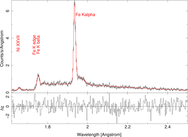
Figure 1.— Chandra HETG spectra of the HMXB GX301$-$2, included in this survey, ObsID 2733, showing all the relevant features discussed in the present work: Fe K$\alpha$ and Fe K$\beta$ fluorescence lines, Fe K edge, Compton shoulder and a hot line.

2. Observations

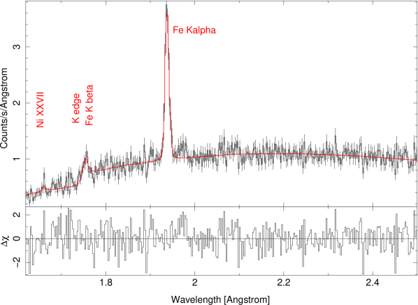
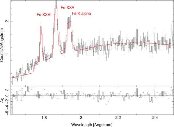
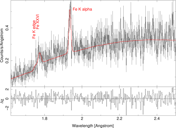
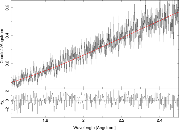
Figure 2.— Four representative examples of the fitting process. Upper row: HMXBs. Left: Vela X-1 shows Fe K$\alpha$ and Fe K$\beta$ but not hot photoionization lines (except Ni xxvii). Right: Cyg X-3, in turn, shows hot photoionization lines of Fe xxv and Fe xxvi which, in low resolution and broadband spectra, are confused with the true cold Fe K$\alpha$ fluorescence line. Lower row: LMXBs. Left: 4U1822$-37$ shows Fe K$\alpha$ and a hot line. Right: The spectra of 4U1957$+$11, as the vast majority of LMXBs, shows no lines at all, in this case superimposed on a pure powerlaw continuum.

We have reprocessed all the available HETGS data for OB stellar systems which in the end involved 10 sources. We also searched for Fe fluorescence emission from 31 LMXB and found 4 cases of late type companions with positive detections. The sample is presented in Table 1. In the case of HMXBs we included observational information of all 10 sources available since we detected line fluorescence in all candidates. In the case of LMXBs we include such information only for those with clear detections, but list all the other targets in the footnote for reference purposes.

Table 1The complete sample of X-ray binaries analyzed in this work.

Source	Alternative name	$\alpha$	$\delta$	MK donor	$d$(kpc)	ObsID
HMXB
Cen X-3	4U 1119-603	11 21 15.78	-60 37 22.7	O6.5II-III	8	705, 1943
OAO1657$-$415	EXO 1657-419	17 00 47.90	-41 40 23	Ofpe	7.1$\pm$1.3	1947
Cyg X-1	4U 1956+35	19 58 21.67	+35 12 05.77	O9.7Iab	2.15$\pm$ 0.07	2415, 3815
Cyg X-3	4U 2030+40	20 32 25.78	+40 57 27.9	WR?	9	425, 426, 1456
X1908$+$075	4U 1909+07	19 10 48	+07 35.9	O7.5-9.5If	7	5476, 5477, 6336
Vela X-1	4U 0900-40	09 02 06.86	-40 33 16.90	B0Iab	1.9$\pm$0.1	102, 1926, 1927, 1928
4U1700$-$37		17 03 56.77	-37 50 38.91	O6.5Iaf	1.7	657
GX301$-$2	4U 1223-62	12 26 37.60	-62 46 14	B1.5Ia+	3${}^{+1}_{-0.5}$	103, 2733, 3433
LMC X-4	4U 0532-66	05 32 49.79	-66 22 13.8	O8III	50	9571, 9573, 9574
$\gamma$ Casa	4U 0054+60	00 56 42.53	+60 43 00.26	B0.5IIIe	0.19	1985
LMXB
4U1822-371		18 25 46.8	-37 06 19	M0V		671
GX1+4	4U 1728-24	17 32 02.16	-24 44 44.02	M5III		2710
Her X-1	4U 1656+35	16 57 49.83	+35 20 32.6	A5V	4.5	2749, 3821, 3822, 4585
						6149, 3821, 6150
Cir X-1	4U 1516-56	15 20 40.874	-57 10 00.26	B5-A0		706, 1700

Note. — Only sources with positive detections have been quoted above. E: Eclipsing binary, P: X-ray pulsar. Sources analyzed with negative detections: LMXB: 2S0918-549, 2S0921-63, 4U1254-690, 4U1543-62, 4U1624-49, 4U1626-67, 4U1636-53, 4U1705-44, 4U1728-16, 4U1728-34, 4U1735-44, 4U1820-30, 4U1822-00, 4U1916-053, 4U1957+11, 4U2127+119, Cyg X-2, EXO0748-676, GRO J1655-40, GRS 1747-312, GRS 1758-258, GX13+1. GX17+2, GX3+1, GX339-4, GX340+0, GX349+2, GX5-1, GX9+1, Ginga1826-238, SAX J1747.0-2853, SAX J1808.4-3658, ScoX-1, Ser X-1, XTE J1118+480, XTE J550-564, XTE J1650-500, XTE J 1746, XTE J1814-338. HMXB: Cyg X-1 ObsIDs 107, 1511, 2741, 2742, 2743, 3407, 3724, Cir X-1 ObsIDs 1905, 1906, 1907, 5478, 6148.

There were a few peculiar sources, such as SS 433 or $\gamma$Cas, in which the Fe K region is dynamically either too complex or where the nature of the source as an accreting source is fundamentally in question. Some sources, like LS5039, LMC X-1 and LMC X-3, were excluded because there was no significant X-ray emission in the K$\alpha$ region under study. There are many observations of Cyg X-1 in the archive, but only two of these showed positive detections of the FeK$\alpha$ line. In this case we list only the ObsIDs where we detected line fluorescence. Likewise, sources presenting only warm absorption lines, like 4U1624$-$49 have also been excluded.

For the present study we focus on the 1.6 - 2.5 Å ($\approx 4.96$ keV - 7.74 keV) spectral region, which contains both Fe K$\alpha$, Fe K$\beta$ emissions and the Fe K edge (Fig.1). Pile up has been found to be negligible in this spectral region except for very few sources not included in this survey. We treat the spectral continuum as local and use a simple powerlaw modified either by an edge at 1.740 Å or a photoelectric absorption (phabs, tbabs). For the latter case we apply solar abundances from Anders & Grevesse (1989) and cross sections from Balucinska-Church & McCammon (1992). Our focus on the local continuum is justified by the fact that the process of inner K shell line fluorescence of neutral matter has a fundamentally different relation to its underlying continuum than in the photoionization of warm plasmas. While the latter requires photoionization energies much lower than the K edge energy to remove electrons down to He-like ions of Fe, it requires photon energies beyond the Fe K edge of 7.1 keV to remove an electron from the K shell of neutral Fe. In this respect, Fe K shell fluorescence is entirely independent of the nature of the X-ray continuum below the Fe K edge ($\lambda>1.74$ Å) which allows us to focus on local continua only. Furthermore, the recovery of the continuum beyond the K edge ($\lambda<1.74$ Å) goes with the power of $\sim 3$ and is, thus, extremely steep, requiring to account for the bulk of absorption of photons only very close to the edge itself. This provides us with both the optical depth of the edge $\tau_{\rm edge}$ and the equivalent column density of the reprocessing material, $N_{\rm H}$. Given the spectral range we have focused on, this latter quantity is measured from the K edge via the assumed abundance of Fe with respect to H. Apart from Fe K$\alpha$ and K$\beta$ emissions, other emission lines from photoionised plasma have been detected in many cases, most prominently at 1.85 Å ($\approx 6.7$ keV, Fe xxv), 1.78 Å ($\approx 6.96$ keV, Fe xxvi Ly $\alpha$), and 1.66 Å ($\approx 7.46$ keV, Ni xxvii Ly $\alpha$). Whenever present, these lines were fitted with Gaussians, to get a good fit in the whole wavelength range, but we do not study them here because they are out of the scope of the present paper. The edge has been fixed at 1.740 Å (=7.125 keV) for all the sources.

In Fig. 2 we present four representative examples of the quality of the fits. The upper row shows two HMXBs of our sample, Vela X-1 (left) and Cygnus X-3 (right). As can be seen, the spectra of Vela X-1 is relatively clean, showing only Fe K$\alpha$, Fe K$\beta$ and the K edge (plus a small hot line beyond the edge). The spectra of Cygnus X-3, in turn, is more complex. It shows two hot lines, Fe xxv and Fe xxvi of photoionized iron. These latter lines, in particular Fe xxv, can not be resolved in low resolution and broad band spectra and are often confused with the true fluorescence Fe K$\alpha$ of (near)neutral iron. Hence the paramount importance of using Chandra for the present survey. The lower row corresponds to two LMXBs within our sample. The case of 4U1822$-$37 (left) shows a morphology similar to that of the HMXBs. The high resolution now enables us to discern the hot line Fe xxvi, at 1.78 Å, of photoionized iron not confusing it with Fe K$\beta$ at 1.75 Å. Finally, we show the example of 4U1957$+$11 (right) which, as the vast majority of LMXBs, does not show any emission line or edge at all. The reduced $\chi^{2}$ is $\approx 1$ in all cases.

The data were rebinned to match the resolution of HEG (0.012 Å FWHM) and MEG (0.023 Å FWHM). Except in a few cases, the line width was not or barely resolved. In those cases we fixed the line width to $\sigma=0.005$ Å. The measured $EW$, though, were found to be independent of this value.

In some sources, a Compton shoulder redward of K$\alpha$ can be discerned. In those cases the shoulder was modeled using Gaussian functions. Shoulder properties are presented in Table 4.

Both HEG and MEG data were analyzed. However, only HEG data were used to derive the line properties. First orders ($m=\pm 1$) were fitted simultaneously and MEG data were checked in all cases for consistency. In cases of low S/N the MEG data were also used to reduce errors. All analyzed sources are listed in Table 1. The spectra and the response files (arf and rmf) were extracted using standard CIAO software (v 4.4) and analyzed with Interactive Spectral Interpretation System (ISIS) v 1.4.9-19 (Houck, 2002).

We emphasize that the present study deals specifically with the narrow Fe K$\alpha$ line, for which the Chandra HETG instrument is specifically well suited. A detailed analysis of the broad component would require simultaneous coverage by other broadband telescopes, like RXTE. To illustrate how, we show in Fig. 3 the HETG spectra of 4U1700$-$37 in the region under study (left). Here however, we have extended the spectral range to allow for the detection of the (putative) broad component. We have fitted the data with an absorbed powerlaw and an Fe line composed by a narrow and a broad component (right). For the broad component we have used the line parameters obtained from a non simultaneous RXTE observation of this source ($E=6.4$ keV, $FWHM=0.47$ keV, $EW=133$ eV, keeping the norm equal for both components). It turns out that the broad component is only required by RXTE-PCA data but not required at all by the Chandra data even though, in principle, the spectral range covered should be enough for this purpose, as can be clearly seen in Fig. 3. A similar effect and discussion can be seen in Hanke et al. (2009). As the vast majority of our sample does not have simultaneous Chandra- RXTE observations, no attempt is made in the present study to involve the spectral continuum in excess of the 4.96–7.74 keV (1.6 – 2.5 Å) band.

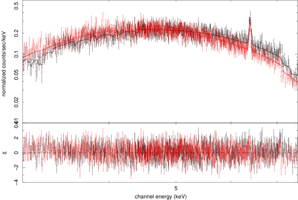
Figure 3.— Left: HETG spectra of the HMXB 4U1700$-$37 for $m=-1$ and $m=+1$ orders. Right: model used to fit the data including a narrow component and a broad component. The parameters of the broad component are taken from a non simultaneous RXTE observation of this source. Its presence though, is not required at all by the Chandra data.

Table 2Parameters for Fe K$\alpha$ fluorescence line

Source	ObsID	$F_{1.6-2.5\rm\AA}$	$F(K\alpha)$	$EW(K\alpha)$	$\lambda_{K\alpha}$	$\tau_{\rm edge}$	$N^{\rm equiv}_{\rm H}$
		$\times 10^{-10}$	$\times 10^{-4}$				$\times 10^{22}$
		(erg s-1 cm-2)	(photons s-1 cm-2)	(eV)	(Å)		(atoms cm-2)
HMXB
OAO1657$-$415	1947	1.09$\pm$0.09	5.20$\pm$2.01	147.09$\pm$56.71	1.9366$\pm$0.0037	1.07$\pm$0.47	55.20$\pm$ 24.34
Cen X-3	705	1.55$\pm$0.03	1.87$\pm$0.50	47.32$\pm$12.52	1.9425$\pm$0.0020	0.62$\pm$0.09	28.81$\pm$ 4.17
	1943	23.14$\pm$2.08	10.69$\pm$1.37	17.43$\pm$2.29	1.9375$\pm$0.0011	0.18$\pm$0.03	11.13$\pm$ 0.92
Cyg X-3	1456	10.36$\pm$2.49	22.00$\pm$2.64	65.28$\pm$7.88	1.9357$\pm$0.0016	0.66$\pm$0.06	28.77$\pm$ 2.60
	425	29.17$\pm$3.50	14.78$\pm$4.35	15.64$\pm$4.61	1.9366$\pm$0.0029	0.34$\pm$0.05	9.82$\pm$ 0.19
	426	26.65$\pm$0.16	18.78$\pm$7.06	21.48$\pm$8.07	1.9398$\pm$0.0057	0.36$\pm$0.05	25.43$\pm$ 2.25
Cyg X-1	3815	27.13$\pm$2.98	16.80$\pm$1.82	19.07$\pm$2.06	1.9397$\pm$0.0018	0.03$\pm$0.01	1.80$\pm$ 0.73
	2415	17.65$\pm$1.68	12.43$\pm$1.72	20.82$\pm$2.05	1.9352$\pm$0.0092	0.07$\pm$0.03	3.31$\pm$1.25
X1908$+$075	6336	0.45$\pm$0.35	1.23$\pm$0.50	81.02$\pm$3.20	1.9375$\pm$0.0038	0.34$\pm$0.09	15.31$\pm$ 4.03
	5476	0.99$\pm$0.03	3.60$\pm$0.67	79.79$\pm$24.85	1.9389$\pm$0.0025	0.10$\pm$0.05	4.02$\pm$ 2.03
	5477	0.34$\pm$0.18	0.69$\pm$0.33	58.06$\pm$26.60	1.9380$\pm$0.0037	0.67$\pm$0.30	29.45$\pm$ 13.13
Vela X-1	1928	11.41$\pm$0.08	20.60$\pm$1.50	53.93$\pm$3.94	1.9375$\pm$0.0004	0.06$\pm$0.04	3.29$\pm$ 2.19
	1927	9.38$\pm$0.14	34.00$\pm$1.73	107.04$\pm$5.50	1.9384$\pm$0.0003	0.38$\pm$0.05	18.55$\pm$ 1.98
	1926	0.08$\pm$0.07	1.94$\pm$0.22	931.51$\pm$112.76	1.9391$\pm$0.0010	0.85$\pm$0.38	34.78$\pm$ 15.51
	102	0.09$\pm$0.08	1.50$\pm$0.39	625.63$\pm$166.80	1.9392$\pm$0.0029	0.70$\pm$0.35	28.49$\pm$ 14.20
4U1700$-$37	657	3.63$\pm$0.04	8.70$\pm$0.81	70.19$\pm$6.45	1.9386$\pm$0.0006	0.30$\pm$0.05	15.03$\pm$ 2.52
GX301$-$2	3433	7.52$\pm$0.05	32.00$\pm$1.14	113.54$\pm$4.08	1.9384$\pm$0.0002	0.48$\pm$0.03	25.15$\pm$ 1.80
	2733	7.52$\pm$0.08	78.15$\pm$3.39	282.68$\pm$3.30	1.9388$\pm$0.0002	1.54$\pm$0.01	82.02$\pm$ 0.53
	103	1.38$\pm$0.07	8.70$\pm$0.91	166.78$\pm$19.65	1.9392$\pm$0.0006	1.22$\pm$0.02	61.82$\pm$ 0.76
LMC X-4	9571	0.31$\pm$0.02	0.83$\pm$0.22	73.71$\pm$21.95	1.9374$\pm$0.0054	0.23$\pm$0.15	9.09$\pm$ 5.00
	9573	0.02$\pm$0.01	0.47$\pm$0.19	890.00$\pm$267.00	1.9422$\pm$0.0056	0.74$\pm$0.35	24.33$\pm$ 12.00
	9574	0.07$\pm$0.01	0.45$\pm$0.25	243.03$\pm$37.74	1.9409$\pm$0.0035	1.43$\pm$0.40	58.42$\pm$ 10.00
$\gamma$ Cas	1985	0.52$\pm$0.01	0.71$\pm$0.27	39.74$\pm$15.04	1.9368$\pm$0.0001	0.57$\pm$0.23	22.76$\pm$1.06
LMXB
4U1822$-$37	671	2.32$\pm$0.53	2.94$\pm$0.69	36.61$\pm$8.52	1.9379$\pm$0.0015	0.31$\pm$0.08	15.52$\pm$3.72
GX1$+$4	2710	0.66$\pm$0.01	1.64$\pm$0.38	72.81$\pm$16.96	1.9376$\pm$0.0013	0.26$\pm$0.19	12.51$\pm$8.62
Her X-1	2749	0.20$\pm$0.03	3.00$\pm$0.40	512.88$\pm$68.98	1.9372$\pm$0.0037	0.38$\pm$0.37	15.26$\pm$15.00
	3821	0.74$\pm$0.16	3.49$\pm$0.74	141.02$\pm$29.76	1.9375$\pm$0.0015	0.48$\pm$0.22	24.32$\pm$10.89
	3822	0.94$\pm$0.63	1.25$\pm$0.83	162.56$\pm$107.94	1.9386$\pm$0.0013	0.70$\pm$0.21	33.84$\pm$10.36
	4585	2.15$\pm$1.15	3.74$\pm$1.41	51.58$\pm$19.46	1.9399$\pm$0.0031	0.64$\pm$0.15	30.79$\pm$7.29
	6149	2.32$\pm$0.53	5.48$\pm$1.26	69.05$\pm$15.88	1.9395$\pm$0.0002	0.45$\pm$0.12	22.42$\pm$6.09
	6150	0.75$\pm$0.20	3.18$\pm$0.85	128.59$\pm$34.29	1.9397$\pm$0.0018	0.74$\pm$0.30	34.58$\pm$14.28
Cir X-1	706	66.31$\pm$4.64	13.94$\pm$ 0.03	6.07$\pm$1.50	1.9392$\pm$0.0018	0.14$\pm$0.02	7.47$\pm$1.23
	1700	36.59$\pm$0.46	17.68$\pm$0.03	14.53$\pm$1.21	1.9388$\pm$0.0019	0.15$\pm$0.03	9.42$\pm$1.35

Note. — Only sources and ObsIDs. with positive detections have been included

Table 3Parameters for Fe K$\beta$ fluorescence line

Source	ObsID	$F(K\beta)(\times 10^{-4})$	$EW(K\beta)$	$\lambda_{K\beta}$
		(photons s-1 cm-2)	(eV)	(Å)
OAO1657$-$415	1947	0.73$\pm$0.73	86.94$\pm$33.52	1.7500$\pm$0.0100
Cen X-3	705	0.25$\pm$0.35	5.90$\pm$2.50	1.7577$\pm$0.0100
Cyg X-1	3815	5.37$\pm$2.48	6.23$\pm$0.67	1.7554$\pm$0.0069
X1908$+$075	6336	1.08$\pm$1.48	77.72$\pm$3.07	1.7464$\pm$0.0057
	5476	1.20$\pm$1.48	41.02$\pm$22.70	1.7453$\pm$0.0051
	5477	0.24$\pm$2.18	17.92$\pm$8.21	1.7471$\pm$0.0076
Vela X-1	1928	4.00$\pm$2.13	11.30$\pm$0.83	1.7597$\pm$0.0034
	1927	3.90$\pm$2.03	11.82$\pm$0.61	1.7556$\pm$0.0037
	1926	0.22$\pm$0.19	95.88$\pm$11.61	1.7553$\pm$0.0099
4U1700$-$37	657	1.40$\pm$1.93	11.06$\pm$1.02	1.7595$\pm$0.0057
GX301$-$2	3433	3.50$\pm$1.17	11.13$\pm$0.40	1.7550$\pm$0.0024
	2733	11.8$\pm$2.45	41.10$\pm$0.48	1.7569$\pm$0.0014
	103	1.32$\pm$0.75	16.07$\pm$1.89	1.7578$\pm$0.0038
LMC X-4	9571	0.09$\pm$0.02	8.39$\pm$1.72	1.7400 (frozen)
	9574	0.19$\pm$ 0.03	72.43$\pm$14.49	1.7528 (frozen)
Her X-1	4585	1.45$\pm$ 0.05	18.51$\pm$2.31	1.7501 (frozen)

3. Results

The results are presented in Tables 2, 3 and 4. They allow for several immediate conclusions to be drawn. Fe fluorescence emission seems to be quite ubiquitous in HMXB. All 10 HMXB analyzed showed fluorescence emission. Those sources with several ObsIDs available show that this emission is highly variable. A particularly striking case is that of Cyg X-1 where only two out of nine observations contained only very weak detections.

In contrast, Fe fluorescence emission seems to be very rare amongst LMXB. Only four LMXB sources out of the 31 analyzed, showed fluorescence line emission. Apart from that, there are no obvious differences in the detected emission levels in LMXB compared with the ones in HMXB. To observe Fe K line fluorescence in $\gtrsim 90\%$ of the HMXB observations, but only in $\gtrsim 10\%$ in LMXBs is in contrast with the finding of Gottwald et al. (1995) and Asai et al. (2000).

The fluorescence Fe K$\alpha$ line is centered at $\lambda_{\rm FeK\alpha}=1.9387\pm 0.0016$ Å, on average, and we do not see significant shifts to higher ionization states. This is equivalent to an energy range from 6.390 - 6.400 keV, consistent with the two components K$\alpha_{1}$ and K$\alpha_{2}$ from ion states below Fe x (House, 1969). These two components are not resolved and the line appears narrow in all cases with $FWHM\lesssim 0.005$ Å, while the lines in Gottwald et al. (1995) and Asai et al. (2000) are of the order of $\sim 0.5-1$ keV. Last, but not least, a Compton shoulder is detected in the only hypergiant source in the sample, GX301-2 (Watanabe et al., 2003) and also in X1908+075, in the latter case, for the first time.

4. Curve of Growth

Figure 4.— The measured fluxes of the Fe K$\beta$ line versus the Fe K$\alpha$ line where both lines could be detected simultaneously. The dashed line represents the theoretical prediction (Palmeri et al., 2003).

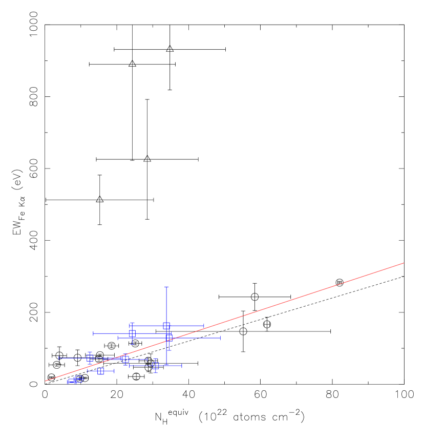
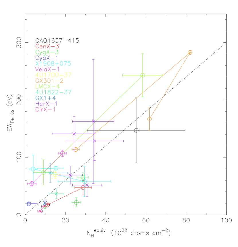
Figure 5.— Left panel: The curve of growth. The $EW$ of the Fe line grows with the column density of the reprocessing material (continuous red line) as predicted by the theoretical model of Kallman et al. (2004) for spherical geometry (dashed line). Black circles represent HMXB data and blue squares represent LMXB. Eclipse data (triangles, upper left corner) do not follow the main trend. Right panel: the several ObsIDs for the same source have been linked by a line, showing that, with few exceptions, the sources follow the relationship individually.

One of the goals of the this study is to establish an empirical relationship between $EW$ of the Fe K$\alpha$ fluorescence line and the column density of the reprocessing material and determine its Curve of Growth. In Fig. 4 we plot the measured fluxes of Fe K$\beta$ versus K$\alpha$ (from data in Tables 2 and 3) for those sources where both lines could be reliably measured simultaneously. As can be seen, the data do not deviate significantly from the theoretical value $F(K\beta)/F(K\alpha)\sim 0.13-0.14$ (Palmeri et al., 2003). Therefore the sample does not show strong evidence of excess resonant Auger destruction and the derived $N_{\rm H}$ will be reliable. The exception is X1908$+$07 for which this ratio seems to be larger. In Fig 5 we plot the curve of growth of the $EW(K\alpha)$ with the H equivalent absorption column of the reprocessing material. As can be seen, the EWs of the Fe K$\alpha$ lines scale linearly with $N_{\rm H}$. The least squares best fit gives

$$EW_{FeK\alpha}({\rm eV})=(3.29\pm 0.05)N^{22}_{\rm H}$$ (1)

where $N^{22}_{\rm H}$ is the equivalent H column of the reprocessing material in units of $10^{22}$ atoms cm^-2. This relationship is plotted as a continuous red line in Fig 5. The degree of correlation is very high (Pearson correlation coefficient of $r=0.95$). We have also plotted the theoretical prediction given by Kallman et al. (2004), Eq.5, namely $EW(FeK\alpha)\simeq 3N^{22}_{\rm H}$ [eV] (black dashed line). The agreement is excellent even though there is a large scatter in the data. This theoretical equation has been computed for spherical geometry and solar abundance. The available data, therefore, are consistent with a spherical distribution of the Fe fluorescence emission zone around the X-ray source. This implies a scenario where the compact object is deeply embedded within the stellar wind of the companion star, as is the likely case in most HMXBs. It is very important to stress that to the most extent, several individual observations of the same object follow this relationship (Fig.5, right panel). The supergiant HMXB X1908$+$07 is an exception and, in fact, shows an anticorrelation. Likewise, no saturation effects are observed within the range of columns studied. Our data in Fig. 5 are also consistent with the lines I and II of Fig. 4 in Inoue (1985) where the reprocessing matter is either spherically distributed around the X-ray source or located between the X-ray source and the observer. Since the compact object is deeply embedded into the wind of the donor, the actual situation is a combination of both. There are points that deviate significantly from this trend (shown as triangles). These points correspond to eclipse data of Vela X-1 and LMC X-4 (ObsId 102, 1926 and 9573 respectively). This can be explained by the computation of the $EW$ (Kallman et al., 2004), which states:

$$EW=\frac{N\omega_{K}y_{Fe}x_{l}}{f_{\epsilon K}}\int_{\epsilon_{\rm Th}}^{\infty}f_{\epsilon}\sigma_{\rm K}(\epsilon)\frac{d\epsilon}{\epsilon}$$ (2)

where $N$ is the radial column density of the reprocessing material, $\omega_{K}$ is the fluorescence yield, $y_{Fe}$ is the Fe elemental abundance, $\sigma_{\rm K}(\epsilon)$ is the K shell photoionization cross section and $f_{\epsilon}$ is the local ionizing continuum. The intensity of the line is normalized to the local continuum, which is strongly suppressed during eclipse. The illuminating source is not observed directly either. The line emitting gas is exposed to the full continuum from the compact object and we see the line emitting gas directly. However, we observe the continuum only via scattering. As a consequence, in eclipse, the very large $EW$ does not correlate well with $N_{\rm H}$. We therefore do not use eclipse points for the subsequent analysis.

Instead of relating the EW and the column density, it might be useful to determine the relationship between the EW and the optical depth at the K edge. From our data we obtain

$$\tau_{K~{}edge}=(0.568\pm 0.005)\left(\frac{EW_{FeK\alpha}}{100\rm~{}eV}\right)$$ (3)

with a Pearson correlation coefficient of $r=0.98$. This equation shows that the reprocessing material reaches optical depth unity for emissions of $EW\sim 175$ eV. Combining Equations 1 and 3 we recover the ISM cross section at the K edge, namely $\sigma_{\rm Fe}=1.8\times 10^{-24}$ cm^-2 (Wilms, Allen and McCray (2000)) as might be expected. It has been shown in Waldron et al. (1998) that the continuum cross section of the wind in OB stars $\sigma_{\rm W}$ is always less than the interstellar value $\sigma_{\rm ISM}$. This is due to the intense UV radiation emitted by the star which increases the ionization state with respect the ISM. This difference is large at low energies while for energies above 1.5 keV ($\lambda\leq 8.3$ Å) we have $\sigma_{\rm W}\approx\sigma_{\rm ISM}$. The fact that we get the ISM value of Wilms, Allen and McCray (2000) is an independent check of the above statement and consistent with the compact object deeply embedded into the wind of the donor.

In conclusion, we find that the curve of growth is consistent with a spherical distribution of reprocessing material around the X-ray source and follows the theoretical prediction of Kallman et al. (2004) (Eq. 5), namely $EW(FeK\alpha)\simeq 3N^{22}_{\rm H}$ [eV]. This is further supported by the fact that the Fe lines are very narrow and in most cases not resolved by Chandra. This means that the material is not rotating at high speeds as would be the case in accretion disks. The few LMXBs follow the same trend as the HMXB. In LMXBs, though, the situation must be different to that in HMXB where the neutron stars are deeply embedded into the stellar winds of their massive companions. To imply a spherical geometry in the LMXB cases is less straight forward but it means that through some mechanism the fluorescing material has lost all ’memory’ of the donor. The eclipse data seem to follow a different relationship with enormous $EW$ which do not match the corresponding large $N_{\rm H}$ deduced from the equation in point 1.

5. On the X-ray Baldwin Effect in XRBs

In Fig. 6 we show the correlation between the unabsorbed continuum flux in the 1.6 - 2.5 Å band, the most effective source for Fe K fluorescence , and the Fe K$\alpha$ line flux. As can be seen , the variations of the reprocessed fluorescence photons track closely the variations of the continuum emitted by the illuminating X-ray source. This means that the reprocessing region must be very close to the X-ray source.

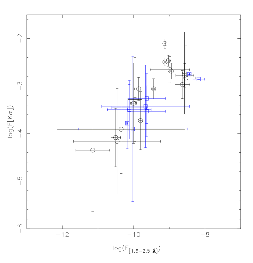
Figure 6.— Log-Log plot of the line flux vs the continuum flux. A good correlation exists ($F_{line}\propto F_{cont}^{0.71};r^{2}=0.75$).The reprocessed fluorescence photons variations track closely the continuum emitted by the X-ray source. This means that the reprocessing region is very close to the X-ray continuum source. Black circles represent HMXB and blue squares LMXB.

While we observe a correlation of line flux with continuum flux, we also observe an anticorrelation of $EW$ with the same continuum flux (Fig. 7). This trend is also visible in the EXOSAT data of Gottwald et al. (1995) (Fig. 3). Such an anticorrelation has been shown to exist for AGNs exhibiting Fe K$\alpha$ fluorescence line (v.g. Iwasawa & Taniguchi (1993), Jiang et al. (2006), Mattson et al. (2007)). This phenomenon is called the ’X-ray Baldwin effect’ following the discovery of a decrease in the EW of the Civ line with increasing UV luminosity in AGNs by Baldwin (1977). Note that in all data sets there is a considerable scatter present. Then we compute the intrinsic $L_{X}$ with the corresponding distance taken from the literature. Even though the trend is still visible, the correlation begins to break down. This can be due to a number of reasons, which may relate to issues such as that the distances for some systems are poorly known, or, as shown recently by Dunn et al. (2008) for GX 339-4, the X-ray Baldwin is effective in the soft state but not in the hard state. Such issues can also contribute to the scatter in Fig. 8. These issues not withstanding, the Chandra data show, for the first time, that such a correlation seems to exist for X-ray binaries in general.

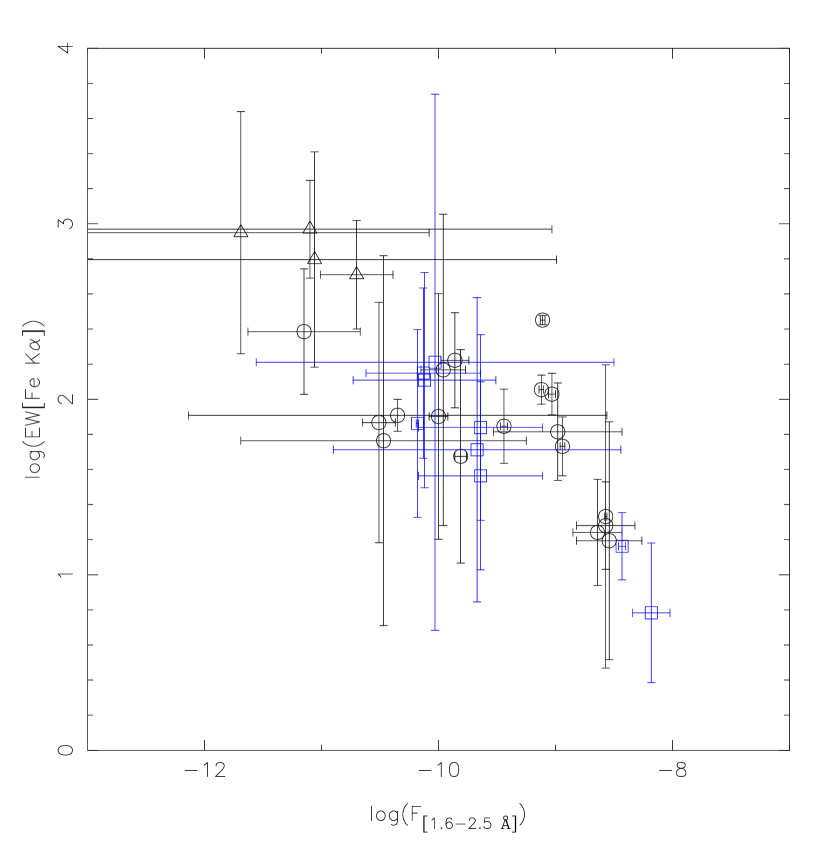
Figure 7.— Log-log plot of the EW of the Fe line vs the unabsorbed flux of the continuum. A clear anticorrelation can be seen. The larger the $F_{X}$ of the central source, the smaller the strength of the line. Black circles represent HMXB, blue squares LMXB and triangles the eclipse data. $EW_{line}\propto F_{cont}^{-0.437};r^{2}=0.80$)

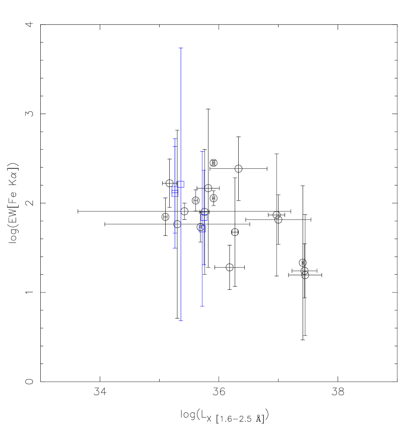
Figure 8.— Baldwin effect for HMXB. Only sources with known distances have been included. A anticorrelation can be seen although the correlation coefficient worsens with respect to that of Fig. 7. This is expected as the larger the $L_{X}$ of the central source, the more ionized is the Fe of the reprocessing region and, therefore, the smaller is the $EW$ of the fluorescence line. Eclipse data have not been plotted. $EW_{line}\propto L_{X}^{-0.289};r^{2}=0.62$)

An immediate interpretation could be ( Nayakshin et al. (2000); Nayakshin (2000)) that upon increase of the continuum X-ray flux from the central source, the surrounding reprocessing material converts from cold, neutral, to progressively ionized with the concurrent decrease in the EW of the fluorescence Fe K$\alpha$ line.

6. Asymmetric lines

Table 4Parameters for Fe K$\alpha$ Compton shoulder

Source	ObsID	$F_{\rm C}(\times 10^{-4})$	$EW_{\rm C}$	$\lambda_{\rm C}$
		(photons s-1 cm-2)	(eV)	(Å)
X1908$+$075	5476	1.74$\pm$0.64	75.91$\pm$27.92	1.9550$\pm$0.0031
GX301$-$2	2733	31.23$\pm$4.68	178.35$\pm$26.75	1.9626$\pm$0.0037
	3433	7.41$\pm$1.27	30.18$\pm$5.17	1.9559$\pm$0.0027

6.1. Compton Shoulders

Within the sample, some sources show asymmetric profiles. We detect a significant shoulder in the supergiant binary X1908$+$075 during ObsId 5476. In Fig. 9 (HEG orders $m=\pm 1$), the Fe K$\alpha$ line shows an extension redward of the main line of $\Delta\lambda\sim 0.06$ Å up to $\sim 2$ Å. The most natural interpretation for this asymmetry is a Compton shoulder. Such features have been resolved with Chandra high resolution capabilities for a small number of extragalactic sources (Kaspi et al., 2002), (Bianchi et al, 2002) and for GX 301-2 (Watanabe et al., 2003). The high energy photons produced in the fluorescence reprocessing region must still traverse the circumsource and circumstellar material to reach the interstellar medium. If this material is Compton thick, the fluorescence photons have a probability of being Compton scattered off electrons with the concurrent decrease in their energy. In Fig. 9 it is clear that primary K$\alpha$ photons are downscattered down to $\sim 2$ Å, i.e. around 0.06 Å. This is exactly the maximum shift $\Delta E_{max}=2E_{0}^{2}/(m_{e}c^{2}+2E_{0})$ with $E_{0}=6.40$ keV (=1.94 Å), for back scattered photons ($\theta=180^{\rm o}$). Therefore, the shoulder is formed through single Compton scattering of the iron K$\alpha$ photons. The apparent concavity of the shoulder is due to the larger probability of forward and backward scatterings which produce minimum and maximum energy shift respectively.

The flux ratio of the shoulder to the primary line is (see Tables 2 and 4) is $\sim 0.48$. This is somewhat higher than the value predicted by Matt (2002). Curiously, the shoulder is not observed during ObsIDs 5477 (high $N_{\rm H}$) and 6336 (medium $N_{\rm H}$). As has been shown by Watanabe et al. (2003) and Matt (2002), too high column densities tend to smear the shoulder as second order scatterings become to be important.

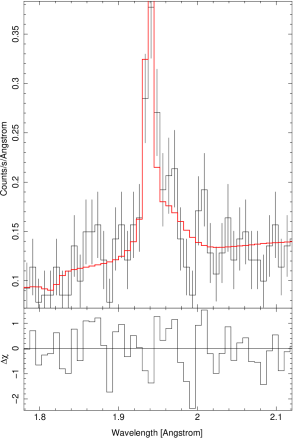
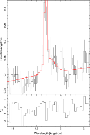
Figure 9.— Compton shoulder seen in X1908$+$075 (ObsId 5476) when the $N_{\rm H}$ is low for $m=-1$ (left) and $m=+1$ (right) orders respectively. The shoulder has been modeled with a simple gaussian and both orders have been fitted together. Parameters are given in Table 4.

6.2. Asymmetric Line Wings

Instead of the clear shoulder displayed in the previous section, some sources present asymmetric wings which include a sharp blue side and an extended, progressive red decline (see Fig. 10).

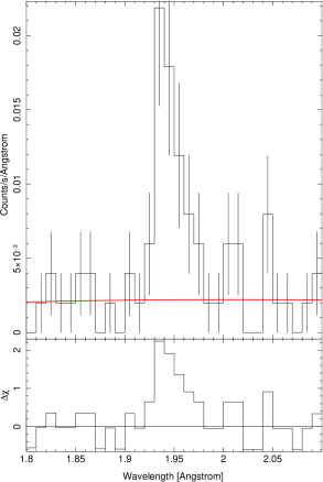
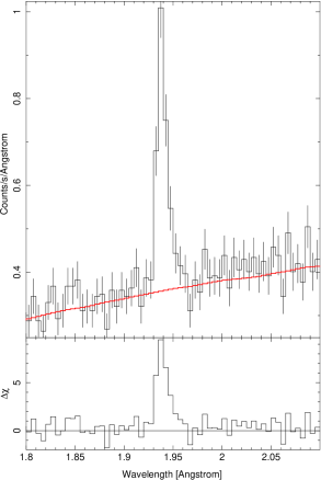
Figure 10.— Asymmetric profiles seen in LMC X-4 ObsId 9573 and 4U1700$-$37 ObsId 657. The local continuum has been modeled with a powerlaw. No gaussians have been added to model the emission line so that the wing is clearly visible in the residuals.

In order to produce Compton shoulders, the scattering gas must be very cold, i.e. less than $\sim 10^{5}$ K. However, anytime the gas is cooler than $\sim E_{K\alpha}/4$, where $E_{K\alpha}$ is the Fe K$\alpha$ line energy, there will be net downscattering. Therefore, these wings could be interpreted as some form of ’hot Compton shoulder’.

Owocki & Cohen (2001) have computed profiles for X-ray lines emitted in the winds of OB stars. They show clearly a characteristic red wing whenever they are produced within the Wind-shock paradigm (see Fig. 4 of that reference), while they tend to show symmetric profiles if the origin is coronal and, thus, produced at or very near the surface of the star. Therefore, the characteristic profile of the lines in Fig. 10 suggests that the Fe K$\alpha$ line is formed in the shocked wind of hot stars illuminated by the X-ray source.

7. Discussion

Figure 11.— RXTE-ASM lightcurve of Cyg X-1. Vertical lines represent the dates of the Chandra pointings included in this survey. Numbers along the lines refer to the corresponding ObsID. Solid lines correspond to positive detections of Fe K$\alpha$ lines while dashed lines correspond to non detections.

Our finding that narrow Fe K lines are present in every HMXB but are very rare in LMXBs is in stark contrast with an early study by Gottwald et al. (1995) and a more recent study by Asai et al. (2000). While in the latter study over about 50$\%$ of line detections were clearly pointing towards the existence of ionized Fe K lines, many detections allowed to be interpreted as Fe line fluorescence. Our analysis, on the other hand, shows that while $\sim 100\%$ of HMXBs show a presence of a narrow line, only less than $\sim 10\%$ of LMXBs do. Likewise, we do not find much Fe K edge absorption in LMXBs. This supports our previous findings and also the conclusion by Miller et al. (2009) that absorption in the interstellar medium dominates the neutral column density observed in LMXB spectra.

Studies of Fe fluorescence in X-ray binaries are not trivial and issues regarding statistics, bandpass, and competing physical processes play a vital role in the interpretation of the results. In general, the process of Fe line fluorescence is bandpass limited to the Fe K line regions unless secondary competing effects exist. This has the advantage that we do not need to deal with broad band binary modelings, which are generally very difficult, uncertain, and even controversial. Our survey, however, can very well discern moderately broadened line emission from neutral and warm Fe K fluorescence (1.94 Å to 1.90 Å) and emission from highly ionized species of Fe XXV (1.85 Å) and Fe XXVI (1.78 Å) much to the level of the ASCA survey by Asai et al. (2000).

Shaposhnikov et al. (2009) found a significantly broadened Fe K line with Suzaku, at medium spectral, resolution with a line width exceeding 10⁴ km s^-1, in the spectrum of Cyg X-2, which was modeled by either a relativistic disk reflection model (Fabian et al., 1982; Laor, 1991) or an extended red-skewing wind model (Laurent & Titarchuk, 2007). The Chandra observation (Schulz et al., 2009) also shows such a broad line, but in contrast resolves the line into the Fe XXV He-like triplet and the Fe XXVI H-like line component ruling out Fe line fluorescence. Clearly, extreme cases of broad line emission as detected in some LMXBs (Bhattacharyya & Strohmayer 2007, Cackett et al. 2008) are difficult, if not impossible, to detect with local continua. However, besides the fact that they are still controversial, they also seem not to be associated with the Fe K edge absorption as the line fluorescence in our survey.

Our study shows that the narrow Fe K lines detected are produced in the relatively cold wind of massive stars by reprocessing the X-ray photons from the X-ray source. The reprocessing material is spherically distributed around the X-ray source leading to narrow FeK$\alpha$ line widths of $FWHM\lesssim 0.005$ Å. For the measured FeK$\alpha$ wavelengths this is equivalent to a velocity $v=c\frac{\Delta\lambda}{\lambda}\approx\frac{FWHM}{\lambda}\approx 770$ km/s. Assuming a typical beta-law, for the velocity of the wind

$$v_{w}=v_{\infty}(1-R_{*}/r)^{\beta}$$

with $\beta=0.8$ and $r$ of the order of $2R_{*}$, we have $v_{w}\sim 0.6v_{\infty}$. Typical terminal velocities for OB stars are of the order of $v_{\infty}=1500$ km/s which yields $v_{w}\simeq 850$ km/s, slightly larger, but of the order of, the width of the observed lines. Thus, the origin of the narrow component is compatible with the stellar wind. Systems with strong winds will present a strong (narrow) Fe K line. It is not present in LMXB except in those rare cases where the system presents a substantial wind component. Indeed, 4U1822$-$371 is the prototypical Accretion Disk Corona source, Cir X-1 presents a hot accretion disk wind (Schulz & Brandt, 2002), GX1$+$4 is a symbiotic binary whose MIII donnor has a powerful wind and Her X-1 has an A type donor, the earliest of the late type companions.

The wind however, can not be the only origin for narrow lines. Indeed, illuminated disks can produce narrow lines, as well, under the right conditions. It has been observed, for example, in the Seyfert 1 galaxy NGC 3783 originating, at least partially, from a relativistic accretion disk (Yaqoob et al., 2005). Since we do not observe this line in LMXBs, either their disks are too hot or not illuminated.

A particularly striking case is that of the HMXB Cyg X-1 where only two, out of nine observations analyzed, have shown Fe K$\alpha$ in emission. In these two cases the emission is amongst the weakest of the whole sample. In Fig. 11 we show all the Chandra pointings overplotted on the RXTE-ASM lightcurve. As can be seen, the two observations where the line has been observed, marked by solid lines, do not correspond to the same spectral state of the source. During the ObsID 2415 observation, the source was in an intermediate state, with $\sim 50$ cps in the ASM. On the other hand, during the ObsID 3815 observation, the source was clearly in a low (hard) state, with $\sim 25$ cps. The lack of detection in the highest states (2741, 2742, 2743, 3407, 3724) could be explained by the Baldwin effect discussed in this paper: the increase of the luminosity of the X-ray source, increases the degree of ionization of the neutral Fe, thereby decreasing the strength of the fluorescence line. This would be supported by the findings by Hanke et al. (2009) and Juett et al. (2004) in which the neutral column densities decrease with increasing luminosity. The lack of detection during ObsIDs 107 (intermediate-low state) and 1511 (low state), can not be explained in this way and is enigmatic. As stated before, (Dunn et al., 2008) have shown that, for the case of GX339$-$4, the Baldwin effect seems to be only effective in the high soft state and not in the low hard state.

Chandra HETG spectra thus proves to be uniquely qualified to separate narrow Fe K line fluorescence from hot and broad line components. Even though HETG spectra detect far less hot Fe K lines in LMXBs than the survey conducted by Asai et al. (2000), this can easily be explained by the intrinsic variability of the the hot component in these sources as well as fitting biases in CCD spectra.

8. Conclusions

We have reprocessed and analyzed the HETG spectra of all X-ray binaries publicly available at the Chandra archive with specific focus on the Fe K line region. The following conclusions can be drawn from this analysis:

Fe $K\alpha$ fluorescence emission seem to be ubiquitous in HMXBs. This emission varies throughout time for a specific source. In particular, Cyg X-1 shows a rather weak emission, only in two out of nine Chandra observations analyzed here. This emission is detected in two different spectral states: during a low hard state (ObsID 3815) and an intermediate state (ObsID 2415). It vanishes for brighter (softer) states. A possible explanation could reside in the X-ray Baldwin effect studied before. Only in low luminosity states there remains a significant fraction of near neutral Fe, although much less than in other binaries of this survey. This remaining neutral Fe, however, becomes ionized in brighter states with the disappearance of the fluorescence line. However, the lack of detection during other intermediate (ObsID 107) and low hard states (ObsID 1511) defies this explanation and means that this can not be the only mechanism at work in this system.

In contrast, such emissions are found to be very rare amongst LMXBs. Only four sources, out of 31 analyzed in this work, display the narrow component of Fe $K\alpha$ in emission: 4U1822-37, GX1+4, Her X-1, and Cir X-1. This lack of narrow iron line is always accompanied by the lack of any detectable K edge. This finding, strongly suggests, that the neutral absorption column in LMXB is dominated by the interstellar medium while in HMXB the local absorption is very significant.

This finding is in contrast with the previous work by Gottwald et al. (1995), based on spectra of lower resolution, where the majority of sources showing Fe line emission were LMXB. Our findings, however, do not contradict the ASCA study of Asai et al 2000 which claim the detection of hot lines in the majority of LMXB. We point out though, that these hot lines are not as frequently observed in Chandra HETG spectra.

The curve of growth ($EW(K\alpha)$ vs $N_{\rm H}$) is fully consistent with a spherical distribution of reprocessing matter, formed by cold near neutral Fe, around the X-ray source. This reprocessing material must be close to the X-ray source, as the line and continuum variations are closely correlated. Those few LMXB displaying Fe $K\alpha$ in emission follow the same correlations found for the HMXB. Since the nature of the winds is very different in LMXB and HMXB this means that the circumsource material has lost all ’memory’ of the donor. This is consistent with a reprocessing site location very close to the compact object.

We observe a moderate anticorrelation between $EW$ and the $L_{\rm X}$ of the source, on average. Some sources follow individually this trend, over timescales from days to months, while other do not. This ’X-ray Baldwin effect’ is reported here for the first time, for the XRBs as a class. The immediate interpretation is the increase in the degree of ionization of Fe with the increasing $L_{\rm X}$ of the illuminating source which produces a concurrent decrease in the efficiency of the fluorescence process.

We observe a Compton shoulder in the supergiant HMXB X1908$+$075 formed by single Compton scattering of primary K$\alpha$ photons. Together with the hypergiant system GX 301-2, where such a shoulder has first been reported (Watanabe et al., 2003), they form the very small group of galactic sources with such a feature detected. Other sources (LMC X-4, 4U1700$-$37) show asymmetric wings, with the blue wings rising sharply and red wings declining progressively. This effect can be explained as ’hot Compton shoulders’.

Fe line fluorescence is produced in the stellar wind of massive stars. Systems with a substantial wind component will show this line. Therefore it can be naturally observed in all HMXB. On the other hand, donor stars in LMXB are not significant sources of stellar winds and other sites must be invoked for the origin of this line. Relativistic accretion disks, as observed in some Seyfert galaxies, might be suitable candidates for those few LMXB with positive detections. However, the lack of the narrow Fe line in the spectra of the vast majority of LMXB might be an indication that such accretion disks are too hot or not illuminated.

References

- Anders & Grevesse (1989) Anders E., Grevesse N. 1989, Geochim. Cosmochim. Acta 53, 197
- Asai et al. (2000) Asai K., Dotani T., Nagase F. Mitsuda K. 2000, ApJS 131, 571
- Baldwin (1977) Baldwin J.A. 1977, ApJ 214, 679
- Balucinska-Church & McCammon (1992) Balucinska-Church, McCammon 1992 ApJ 400, 699
- Battacharya & Strohmayer (2007) Battacharya, Strohmayer T. 2007 ApJ 664 L103
- Bianchi et al (2002) Bianchi S., Matt G., Fiore F., Fabian A.C., Iwasawa K., Nicastro F. 2002, A&A 396, 793
- Cackett et al. (2008) Cackett E.M., Miller J.M., Bhattacharyya S. et al. 2008, ApJ 674, 415
- Canizares et al. (2005) Canizares C.R. et al 2005, PASP 117, 1144
- Dunn et al. (2008) Dunn R.J.H., Fender R.P., Körding E.G., Cabanac C. and Belloni T. 2008, MNRAS 387, 545
- Fabian et al. (1982) Fabian A. C., Rees M. J., Stella L., White N.E. 1989, MNRAS 238, 729
- George & Fabian (1991) George I.M., Fabian A.C. 1991, MNRAS 249, 352
- Gottwald et al. (1995) Gottwald M., Parmar A. N., Reynolds A.P., White N.E. Peacock A., Taylor B.G. 1995, A&AS 109, 9
- Hanke et al. (2009) Hanke M., Wilms J., Nowak M.A., Pottschmidt K., Schulz N.S., Lee J.C. 2009 ApJ 690. 330
- Hatchett & Weaver (1977) Hatchett S., Weaver R. 1977, ApJ 215, 285
- Houck (2002) Houck J.C. 2002, in High Resolution X-ray Spectrsocopy with XMM-Newton and Chandra, ed. G. Branduarni-Raymont
- House (1969) House L.L. 1969, ApJS 18, 21
- Inoue (1985) Inoue H. 1985 SSRv 40, 317
- Iwasawa & Taniguchi (1993) Iwasawa K., Taniguchi Y. 1993, ApJ 413, L15
- Jiang et al. (2006) Jiang P., Wang J.X., Wang T.G. 2006, ApJ 644, 725
- Juett et al. (2004) Juett A.M., Schulz N.S., Chakrabarty D. 2004, ApJ 612, 308
- Kaastra & Mewe (1993) Kaastra J.S., Mewe R. 1993, A&AS 97, 443
- Kallman et al. (2004) Kallman, T. Palmieri, P., Bautista M.A., Mendoza C., Krolik J.H. 2004, ApJS, 155, 675
- Kaspi et al. (2002) Kaspi S., Brandt W.N., George I. M. et al. 2002, ApJ 574, 643
- Laor (1991) Laor A., 1991, ApJ 376, 90
- Laurent & Titarchuk (2007) Laurent P., Titarchuk L. 2007, ApJ 656, 1056
- Matt (2002) Matt G. 2002, MNRAS 337, 147
- Mattson et al. (2007) Mattson B.J., Weaver K.A., Reynolds C.S. 2007, ApJ 664, 101
- Morrison & McCammon (1983) Morrison R, McCammon D. 1983, ApJ 270, 119
- Miller et al. (2002) Miller J.M., Fabian A.C., Wijnands R., Remillard R.A., Wojdowski P., Schulz N.S., Di Matteo T., Marshall H.L., Canizares, C.R., Pooley D., Lewin W.H.G., 2002, ApJ 578, 348
- Miller et al. (2009) Miller J.M., Cackett E.M., Reiss 2009 ApJ 707, L77
- Nayakshin et al. (2000) Nayakshin S. Kazanas S., Kallman T. 1999, ApJ 537, 833
- Nayakshin (2000) Nayakshin S. 2000, ApJ 534, 718
- Owocki & Cohen (2001) Owocki S.P., Cohen D.H. 2001, ApJ 559, 1108
- Palmeri et al. (2003) Palmeri P., Mendoza C., Kallman T.R., Bautista M.A., Meléndez M. 2003, A&A 410, 359
- Reynolds & Nowak (2003) Reynolds C.S., Nowak M. A. 2003, Physics Reports 377, 389