Complexity Analysis of Balloon Drawing for Rooted Trees

Abstract

In a balloon drawing of a tree, all the children under the same parent are placed on the circumference of the circle centered at their parent, and the radius of the circle centered at each node along any path from the root reflects the number of descendants associated with the node. Among various styles of tree drawings reported in the literature, the balloon drawing enjoys a desirable feature of displaying tree structures in a rather balanced fashion. For each internal node in a balloon drawing, the ray from the node to each of its children divides the wedge accommodating the subtree rooted at the child into two sub-wedges. Depending on whether the two sub-wedge angles are required to be identical or not, a balloon drawing can further be divided into two types: even sub-wedge and uneven sub-wedge types. In the most general case, for any internal node in the tree there are two dimensions of freedom that affect the quality of a balloon drawing: (1) altering the order in which the children of the node appear in the drawing, and (2) for the subtree rooted at each child of the node, flipping the two sub-wedges of the subtree. In this paper, we give a comprehensive complexity analysis for optimizing balloon drawings of rooted trees with respect to angular resolution, aspect ratio and standard deviation of angles under various drawing cases depending on whether the tree is of even or uneven sub-wedge type and whether (1) and (2) above are allowed. It turns out that some are NP-complete while others can be solved in polynomial time. We also derive approximation algorithms for those that are intractable in general.

1 Introduction

Graph drawing addresses the issue of constructing geometric representations of graphs in a way to gain better understanding and insights into the graph structures. Surveys on graph drawing can be found in [1, 6]. If the given data is hierarchical (such as a file system), then it can often be expressed as a rooted tree. Among existing algorithms in the literature for drawing rooted trees, the work of [11] developed a popular method for drawing binary trees. The idea behind [11] is to recursively draw the left and right subtrees independently in a bottom-up manner, then shift the two drawings along the $x$-direction as close to each other as possible while centering the parent of the two subtrees one level up between their roots. Different from the conventional ‘triangular’ tree drawing of [11], $hv$-drawings [12], radial drawings [3] and balloon drawings [2, 4, 7, 9, 10] are also popular for visualizing hierarchical graphs. Since the majority of algorithms for drawing rooted trees take linear time, rooted tree structures are suited to be used in an environment in which real-time interactions with users are frequent.

Consider Figure 1 for an example. A balloon drawing [2, 4, 9] of a rooted tree is a drawing having the following properties:

• all the children under the same parent are placed on the circumference of the circle centered at their parent;

• there exist no edge crossings in the drawing;

• the radius of the circle centered at each node along any path from the root node reflects the number of descendants associated with the node (i.e., for any two edges on a path from the root node, the farther from the root an edge is, the shorter its drawing length becomes).

In the balloon drawing of a tree, each subtree resides in a wedge whose end-point is the parent node of the root of the subtree. The ray from the parent node to the root of the subtree divides the wedge into two sub-wedges. Depending on whether the two sub-wedge angles are required to be identical or not, a balloon drawing can further be divided into two types: drawings with even sub-wedges (see Figure 1(a)) and drawings with uneven sub-wedges (see Figure 1(b)). One can see from the transformation from Figure 1(a) to Figure 1(b) that a balloon drawing with uneven sub-wedges is derived from that with even sub-wedges by shrinking the drawing circles in a bottom-up fashion so that the drawing area is as small as possible [9]. Another way to differentiate the two is that for the even sub-wedge case, it is required that the position of the root of a subtree coincides with the center of the enclosing circle of the subtree.

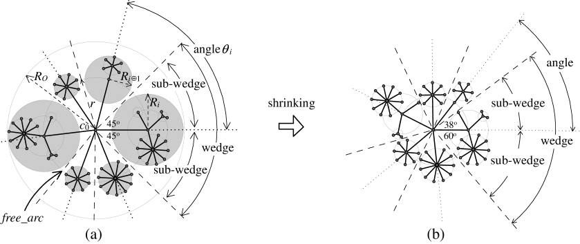
Figure 1: Illustration of balloon drawings with (a) even sub-wedges and (b) uneven sub-wedges, where each node is drawn by a point; each edge is drawn by a solid straight line segment; the center of the largest circle in a balloon drawing is the root node.

Aesthetic criteria specify graphic structures and properties of drawing, such as minimizing number of edge crossings or bends, minimizing area, and so on, but the problem of simultaneously optimizing those criteria is, in many cases, NP-hard. The main aesthetic criteria on the angle sizes in balloon drawings are angular resolution, aspect ratio, and standard deviation of angles. Note that this paper mainly concerns the angle sizes, while it is interesting to investigate other aesthetic criteria, such as the drawing area, total edge length, etc. Given a drawing of tree $T$, an angle formed by the two adjacent edges incident to a common node $v$ is called an angle incident to node $v$. Note that an angle in a balloon drawing consists of two sub-wedges which belong to two different subtrees, respectively (see Figure 1). With respect to a node $v$, the angular resolution is the smallest angle incident to node $v$, the aspect ratio is the ratio of the largest angle to the smallest angle incident to node $v$, and the standard deviation of angles is a statistic used as a measure of the dispersion or variation in the distribution of angles, equal to the square root of the arithmetic mean of the squares of the deviations from the arithmetic mean.

The angular resolution (resp., aspect ratio; standard deviation of angles) of a drawing of $T$ is defined as the minimum angular resolution (resp., the maximum aspect ratio; the maximum standard deviation of angles) among all nodes in $T$. The angular resolution (resp., aspect ratio; standard deviation of angles) of a tree drawing is in the range of $(0^{\circ},360^{\circ})$ (resp., $[1,\infty)$ and $[0,\infty)$). A tree layout with a large angular resolution can easily be identified by eyes, while a tree layout with a small aspect ratio or standard deviation of angles often enjoys a very balanced view of tree drawing. It is worthy of pointing out the fundamental difference between aspect ratio and standard deviation. The aspect ratio only concerns the deviation between the largest and the smallest angles in the drawing, while the standard deviation deals with the deviation of all the angles.

With respect to a balloon drawing of a rooted tree, changing the order in which the children of a node are listed or flipping the two sub-wedges of a subtree affects the quality of the drawing. For example, in comparison between the two balloon drawings of a tree under different tree orderings respectively shown in Figures 2(a) and 2(b), we observe that the drawing in Figure 2(b) displays little variations of angles, which give a very balanced drawing. Hence some interesting questions arise: How to change the tree ordering or flip the two sub-wedge angles of each subtree such that the balloon drawing of the tree has the maximum angular resolution, the minimum aspect ratio, and the minimum standard deviation of angles?

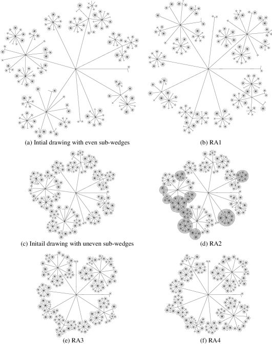
Figure 2: An experimental example, where (a) and (c) are initial balloon drawings with even and uneven sub-wedges, respectively; (b), (d), (e) and (f) achieve the optimality of RA1, RA2, RA3 and RA4, respectively. Note that the differences of (d) from (c) are encompassed by shaded regions.

Throughout the rest of this paper, we let RE, RA, and DE denote the problems of optimizing angular resolution, aspect ratio, and standard deviation of angles, respectively. In this paper, we investigate the tractability of the RE, RA, and DE problems in a variety of cases, and our main results are listed in Table 1, in which trees with ‘flexible’ (resp., ‘fixed’) uneven sub-wedges refer to the case when sub-wedges of subtrees are (resp., are not) allowed to flip; a ‘semi-ordered’ tree is an unordered tree where only the circular ordering of the children of each node is fixed, without specifying if this ordering is clockwise or counterclockwise in the drawing. Note that a semi-ordered tree allows to flip uneven sub-wedges in the drawing, because flipping sub-wedges of a node in the bottom-up fashion of the tree does not modify the circular ordering of its children. See Figure 2 for an experimental example with the drawings which achieve the optimality of RA1–RA4. In Table 1, with the exception of RE1 and RA1 (which were previously obtained by Lin and Yen in [9]), all the remaining results are new. We also give 2-approximation algorithms for RA3 and RA4, and $O(\sqrt{n})$-approximation algorithms for DE3 and DE4. Finding improved approximation bounds for those intractable problems remains an interesting open question.

Table 1: The time complexity for optimizing main aesthetic criteria of balloon drawing.

case		aesthetic criterion	denotation	complexity	reference
C1:	unordered trees with	angular resolution	RE1	$O(n\log n)$	[9]
	even sub-wedges	aspect ratio	RA1	$O(n\log n)$	[9]
		standard deviation	DE1	$O(n\log n)$∗	[Thm 1]
C2:	semi-ordered trees with	angular resolution	RE2	$O(n)$∗	[Thm 2]
	flexible uneven sub-wedges	aspect ratio	RA2	$O(n^{2})$∗	[Thm 3]
		standard deviation	DE2	$O(n)$∗	[Thm 4]
C3:	unordered trees with	angular resolution	RE3	$O(n\log n)$∗	[Thm 5]
	fixed    uneven sub-wedges	aspect ratio	RA3	NPC∗	[Thm 6, 8]
		standard deviation	DE3	NPC∗	[Thm 7, 10]
C4:	unordered trees with	angular resolution	RE4	$O(n\log n)$∗	[Thm 5]
	flexible uneven sub-wedges	aspect ratio	RA4	NPC∗	[Thm 6, 8]
		standard deviation	DE4	NPC∗	[Thm 7, 10]

^∗The marked entries are the contributions of this paper. Note that earlier results reported in [9] for RE2 and RA2 require $O(n^{2.5})$ time.

The rest of the paper is organized as follows. Some preliminaries are given in Section 2. The problems for cases C1 and C2 are investigated in Section 3. The problems for cases C3 and C4 are investigated in Section 4. The approximation algorithms for those intractable problems are given in Section 5. Finally, a conclusion is given in Section 6.

2 Preliminaries

In this section, we first introduce two conventional models of balloon drawing, then define our concerned problems, and finally introduce some related problems.

2.1 Two Models of Balloon Drawing

There exist two models in the literature for generating balloon drawings of trees. Given a node $v$, let $r(v)$ be the radius of the drawing circle centered at $v$. If we require that $r(v)$ = $r(w)$ for arbitrary two nodes $v$ and $w$ that are of the same depth from the root of the tree, then such a drawing is called a balloon drawing under the fractal model [7]. The fractal drawing of a tree structure means that if $r_{m}$ and $r_{m-1}$ are the lengths of edges at depths $m$ and $m-1$, respectively, then $r_{m}=\gamma\times r_{m-1}$ where $\gamma$ is the predefined ratio ($0<\gamma<1$) associated with the drawing under the fractal model. Clearly, edges at the same depth have the same length in a fractal drawing.

Unlike the fractal model, the subtrees with nonuniform sizes (abbreviated as SNS) model [2, 4] allows subtrees associated with the same parent to reside in circles of different sizes (see also Figure 1(a)), and hence the drawing based on this model often results in a clearer display on large subtrees than that under the fractal model. Given a rooted ordered tree $T$ with $n$ nodes, a balloon drawing under the SNS model can be obtained in $O(n)$ time (see [2, 4]) in a bottom-up fashion by computing the edge length $r$ and the angle $\theta_{i}$ between two adjacent edges respectively according to $r=C/(2\pi)\cong(2\sum\nolimits_{i}R_{i})/(2\pi)$ and $\theta_{i}\cong(R_{i}+free\_arc+R_{i+1})/r$ (see Figure 1(a)) where $r$ is the radius of the inner circle centered at node $c_{0}$; $C$ is the circumference of the inner circle; $R_{i}$ is the radius of the outer circle enclosing all subtrees of the $i$-th child of $c_{0}$, and $R_{O}$ is the radius of the outer circle enclosing all subtrees of $c_{0}$; since there exists a gap between $C$ and the sum of all diameters, we can distribute to every $\theta_{i}$ the gap between them evenly, which is called a free arc, denoted by $free\_arc$.

Note that the balloon drawing under the SNS model is our so-called balloon drawing with even sub-wedges. A careful examination reveals that the area of a balloon drawing with even sub-wedges (generated by the SNS model) may be reduced by shrinking the free arc between each pair of subtrees and shortening the radius of each inner circle in a bottom-up fashion [9], by which we can obtain a smaller-area balloon drawing with uneven sub-wedges (e.g., see the transformation from Figure 1(a) to Figure 1(c)).

2.2 Notation and Problem Definition

In what follows, we introduce some notation, used in the rest of this paper. A circular permutation $\pi$ is expressed as: $\pi=\langle\pi_{1},\pi_{2},...,\pi_{n}\rangle$ where for $i=1,2,...,n$, $\pi_{i}$ is placed along a circle in a counterclockwise direction. Note that $\pi_{n}$ is adjacent to $\pi_{1}$; $i\oplus 1$ denotes $i+1\ (mod\ n)$; $i\ominus 1$ denotes $i-1\ (mod\ n)$. Due to the hierarchical nature of trees and the ways the aesthetic criteria (measures) for balloon drawings are defined, an algorithm optimizing a star graph can be applied repeatedly to a general tree in a bottom-up fashion [9], yielding an optimum solution with respect to a given aesthetic criterion. Thus, it suffices to consider the balloon drawing of a star graph when we discuss these problems.

A star graph is characterized by a root node $c_{0}$ together with its $n$ children $c_{1},...,c_{n}$, each of which is the root of a subtree located entirely in a wedge, as shown in Figure 1(a) (for the even sub-wedge type) and Figure 3 (for the uneven sub-wedge type). In what follows, we can only see Figure 3 because the even sub-wedge type can be viewed as a special case of the uneven sub-wedge type. The ray from $c_{0}$ to $c_{i}$ further divides the associated wedge into two sub-wedges $SW_{i,0}$ and $SW_{i,1}$ with sizes of angles $w_{0}(i)$ and $w_{1}(i)$, respectively. Note that $w_{0}(i)$ and $w_{1}(i)$ need not be equal in general. An ordering of $c_{0}$’s children is simply a circular permutation $\sigma=\langle\sigma_{1},\sigma_{2},...,\sigma_{n}\rangle$, in which $\sigma_{i}\in\{1,2,...,n\}$ for each $i$.

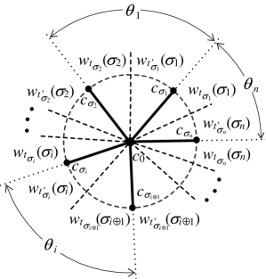
Figure 3: Notations used in a balloon drawing of a star graph with uneven sub-wedges.

There are two dimensions of freedom affecting the quality of a balloon drawing for a star graph. The first is concerned with the ordering in which the children of the root node $c_{0}$ are drawn. With a given ordering, it is also possible to alter the order of occurrences of the two sub-wedges associated with each child of the root. With respect to child $c_{i}$ and its two sub-wedges $SW_{i,0}$ and $SW_{i,1}$, we use $t_{i}\in\{0,1\}$ to denote the index of the first sub-wedge encountered in a counterclockwise traversal of the drawing. For convenience, we let $t^{\prime}_{i}=1-t_{i}$. We also write $t=(t_{1},...,t_{n})$ ($t_{i}\in\{0,1\},1\leq i\leq n$), which is called the sub-wedge assignment (or simply assignment). As shown in Figure 3, the sequence of sub-wedges encountered along the cycle centered at $c_{0}$ in a counterclockwise direction can be expressed as:

$$\begin{array}[]{ccccc}\langle\ \underbrace{w_{t_{\sigma_{1}}}(\sigma_{1}),w_{t^{\prime}_{\sigma_{1}}}(\sigma_{1})},&...,&\underbrace{w_{t_{\sigma_{i}}}(\sigma_{i}),w_{t^{\prime}_{\sigma_{i}}}(\sigma_{i})},&...,&\underbrace{w_{t_{\sigma_{n}}}(\sigma_{n}),w_{t^{\prime}_{\sigma_{n}}}(\sigma_{n})}\ \rangle.\\ c_{\sigma_{1}}&...&c_{\sigma_{i}}&...&c_{\sigma_{n}}\end{array}$$ (3)

If $w_{0}(i)=w_{1}(i)$ for each $i\in\{1,...,n\}$, then the drawing is said to be of even sub-wedge type; otherwise, it is of uneven sub-wedge type. As mentioned earlier, the order of the two sub-wedges associated with a child (along the counterclockwise direction) affects the quality of a drawing in the uneven sub-wedge case. For the case of uneven sub-wedge type, if the assignment $t$ is given a priori, then the drawing is said to be of fixed uneven sub-wedge type; otherwise, of flexible uneven sub-wedge type (i.e., $t$ is a design parameter).

As shown in Figure 3, with respect to an ordering $\sigma$ and an assignment $t$ in circular permutation (3), $c_{\sigma_{i}}$ and $c_{\sigma_{i\oplus 1}}$, $1\leq i\leq n$, are neighboring nodes, and the size of the angle formed by the two adjacent edges $\overrightarrow{c_{0}c_{\sigma_{i}}}$ and $\overrightarrow{c_{0}c_{\sigma_{i\oplus 1}}}$ is $\theta_{i}=w_{t_{i}^{\prime}}(\sigma_{i})+w_{t_{i\oplus 1}}(\sigma_{i\oplus 1})$. Hence, the angular resolution (denoted by $AngResl_{\sigma,t}$), the aspect ratio (denoted by $AspRatio_{\sigma,t}$), and the standard deviation of angles (denoted by $StdDev_{\sigma,t}$) can be formulated as

$$AngResl_{\sigma,t}=\min_{1\leq i\leq n}\theta_{i}=\min_{1\leq i\leq n}\{w_{t_{i}^{\prime}}(\sigma_{i})+w_{t_{i\oplus 1}}(\sigma_{i\oplus 1})\};$$

$$AspRatio_{\sigma,t}=\frac{\max_{1\leq i\leq n}\theta_{i}}{\min_{1\leq i\leq n}\theta_{i}}=\frac{\max_{1\leq i\leq n}\{w_{t_{i}^{\prime}}(\sigma_{i})+w_{t_{i\oplus 1}}(\sigma_{i\oplus 1})\}}{\min_{1\leq i\leq n}\{w_{t_{i}^{\prime}}(\sigma_{i})+w_{t_{i\oplus 1}}(\sigma_{i\oplus 1})\}};$$

$$StdDev_{\sigma,t}=\sqrt{\frac{\sum_{i=1}^{n}\theta_{i}^{2}}{n}-\left(\frac{\sum_{i=1}^{n}\theta_{i}}{n}\right)^{2}}$$

$$=\sqrt{\frac{\sum_{i=1}^{n}(w_{t_{i}^{\prime}}(\sigma_{i})^{2}+w_{t_{i\oplus 1}}(\sigma_{i\oplus 1})^{2})}{n}+\frac{2\sum_{i=1}^{n}w_{t_{i}^{\prime}}(\sigma_{i})w_{t_{i\oplus 1}}(\sigma_{i\oplus 1})}{n}-\left(\frac{2\pi}{n}\right)^{2}}.$$ (4)

We observe that the first and third terms inside the square root of the above equation are constants for any circular permutation $\sigma$ and assignment $t$, and hence, the second term inside the square root is the dominant factor as far as $StdDev_{\sigma,t}$ is concerned. We denote by $SOP_{\sigma,t}$ the sum of products of sub-wedges, which can be expressed as:

$$SOP_{\sigma,t}=\sum_{i=1}^{n}w_{t_{i}^{\prime}}(\sigma_{i})w_{t_{i\oplus 1}}(\sigma_{i\oplus 1}).$$

We are now in a position to define the RE, RA and DE problems in Table 1 for four cases (C1, C2, C3, and C4) in a precise manner. The four cases depend on whether the circular permutation $\sigma$ and the assignment $t$ in a balloon drawing are fixed (i.e., given a priori) or flexible (i.e., design parameters). For example, case C3 allows an arbitrary ordering of the children (i.e., the tree is unordered), but the relative positions of the two sub-wedges associated with a child node are fixed (i.e., flipping is not allowed). The remaining three cases are easy to understand.

We consider the most flexible case, namely, C4, for which both $\sigma$ and $t$ are design parameters, which can be chosen from the set $\Sigma$ of all circular permutations of $\{1,...,n\}$ and the set $\mathbb{T}$ of all $n$-bit binary strings, respectively. The RE and RA problems, respectively, are concerned with finding $\sigma$ and $t$ to achieve the following:

$$optAngResl=\max_{\sigma\in\Sigma;t\in\mathbb{T}}\{AngResl_{\sigma,t}\};optAspRatio=\min_{\sigma\in\Sigma;t\in\mathbb{T}}\{AspRatio_{\sigma,t}\}\texttt{.}$$

The DE problem is concerned with finding $\sigma$ and $t$ to achieve the following:

$$optStdDev = \min_{\sigma\in\Sigma;t\in\mathbb{T}}\{StdDev_{\sigma,t}\}\mbox{}.$$

As stated earlier, $optStdDev$ is closely related to the SOP problem, which is concerned with finding $\sigma$ and $t$ to achieve the following:

$$optSOP = \min_{\sigma\in\Sigma;t\in\mathbb{T}}\{SOP_{\sigma,t}\}.$$

2.3 Related Problems

Before deriving our main results, we first recall two problems, namely, the two-station assembly line problem (2SAL) and the cyclic two-station workforce leveling problem (2SLW) that are closely related to our problems of optimizing balloon drawing under a variety of aesthetic criteria. Consider a serial assembly line with two stations, say $ST_{1}$ and $ST_{2}$, and a set $\mathbb{J}=\{J_{1},J_{2},...,J_{n}\}$ of $n$ jobs. Each job $J_{i}=(W_{i1},W_{i2})$ consists of two tasks processed by the two stations, respectively, where $W_{i1}$ (resp., $W_{i2}$) is the workforce requirement at $ST_{1}$ (resp., $ST_{2}$). Assume the processing time of each job at each station is the same, say $\tau/n$. Consider a circular permutation $\langle J_{\delta_{1}},J_{\delta_{2}},...,J_{\delta_{n}}\rangle$ of $\mathbb{J}$ where $\delta=\langle\delta_{1},\delta_{2},...,\delta_{n}\rangle$ is a circular permutation of $\{1,2,...,n\}$. At any time point, a single station can only process one job. We also assume that the two stations are always busy. During the first time range $[0,\tau/n]$, $J_{\delta_{1}}$ and $J_{\delta_{2}}$ are processed by $ST_{2}$ and $ST_{1}$, respectively, and the workforce requirement is $W_{\delta_{1}2}+W_{\delta_{2}1}$. Similarly, for each $i$, during the time range $[(i-1)\tau/n,i\tau/n]$, $J_{\delta_{i}}$ and $J_{\delta_{i\oplus 1}}$ are processed at $ST_{2}$ and $ST_{1}$ stations respectively, and the workforce requirement is $W_{\delta_{i}2}+W_{\delta_{i\oplus 1}1}$.

For example, consider $\mathbb{J}=\{J_{1},J_{2},J_{3},J_{4}\}$ where $J_{1}=(2,3)$, $J_{2}=(1,7)$, $J_{3}=(6,2)$, and $J_{4}=(4,2)$. For a certain circular permutation $\langle J_{3},J_{2},J_{4},J_{1}\rangle$ of $\mathbb{J}$, the workforce requirements for each period of time as well as the jobs served at the two stations are given in Figure 4, where the largest workforce requirement is 11; the range of the workforce requirements among all the time periods is [3,11].

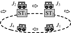
time range	$ST_{1}$	$ST_{2}$	workforce requirement
$[~{}~{}~{}~{}0,~{}\tau/4]$	$J_{2}$	$J_{3}$	$2+1=~{}3$
$[~{}\tau/4,2\tau/4]$	$J_{4}$	$J_{2}$	$7+4=11$
$[2\tau/4,3\tau/4]$	$J_{1}$	$J_{4}$	$2+2=~{}4$
$[3\tau/4,4\tau/4]$	$J_{3}$	$J_{1}$	$3+6=~{}9$

Figure 4: An example for 2SAL and 2SLW.

The $2SAL$ and $2SLW$ problems are defined as follows:

• 2SAL: Given a set of $n$ jobs, find a circular permutation of the $n$ jobs such that the largest workforce requirement is minimized.

• 2SLW (decision version): Given a set of $n$ jobs and a range $[LB,UB]$ of workforce requirements, decide whether a circular permutation exists such that the workforce requirement for each time period is between $LB$ and $UB$.

It is known that 2SAL is solvable in $O(n\log n)$ time [8], while 2SLW is NP-complete [13].

3 Cases C1 (Unordered Trees with Even Sub-Wedges) and C2 (Semi-Ordered Trees with Flexible Uneven Sub-Wedges)

First of all, we investigate the DE1 problem (SOP1 problem), i.e., finding a balloon drawing optimizing $optSOP$ for case C1 (i.e., unordered trees with even sub-wedges). In this case, the two sub-wedges associated with a child node in a star graph are of the same size. For notational convenience, we order the set of wedge angles $\{w_{0}(i)+w_{1}(i):i=1,\cdots,n\}$ (note that in this case $w_{0}(i)=w_{1}(i)$ for each $i$) in ascending order as either

$$m_{1},m_{2},\cdots,m_{k-1},m_{k},M_{k},M_{k-1},\cdots,M_{2},M_{1} n=2k$$ if , or (5)

$$m_{1},m_{2},\cdots,m_{k-1},m_{k},mid,M_{k},M_{k-1},\cdots,M_{2},M_{1} n=2k+1$$ if , (6)

for some $k$, where $m_{i}$ (resp., $M_{i}$) is the $i$-th minimum (resp., maximum) among all, and $mid$ is the median if the number of elements is odd. Note that the size of each angle between two edges in the drawing may be one of the forms $(m_{a}+m_{b})/2$, $(m_{a}+M_{b})/2$, $(M_{a}+m_{b})/2$, or $(M_{a}+M_{b})/2$ for some $a,b\in\{1,\cdots,n\}$, and hence, there may exist more than one angle with the same value. In what follows, we are able to solve the DE1 problem by applying Procedure 1.

Procedure 1 OptBalloonDrawing-DE1

Input: a star graph $S$ with $n$ child nodes of nonuniform sizes
Output: a balloon drawing of $S$ optimizing standard deviation of angles

1:  sort $\{w_{0}(i)+w_{1}(i):i=1,\cdots,n\}$ in ascending order as either Equation (5), if $n=2k$, or Equation (6), if $n=2k+1$

2:  for convenience, let the child node with wedge $m_{i}$, $mid$ or $M_{i}$ be also denoted by $m_{i}$, $mid$ or $M_{i}$, respectively

3:  if $n=2k$ then

4:    if $k$ is odd then

5:       output $\langle M_{1},m_{2},M_{3},m_{4},\cdots,M_{k-1},m_{k},M_{k},m_{k-1},\cdots,M_{4},m_{3},M_{2},m_{1}\rangle$

6:    else

7:       output $\langle M_{1},m_{2},M_{3},m_{4},\cdots,m_{k-1},M_{k},m_{k},M_{k-1},\cdots,M_{4},m_{3},M_{2},m_{1}\rangle$

8:    end if

9:  else

10:    if $k$ is odd then

11:       output $\langle M_{1},m_{2},M_{3},m_{4},\cdots,M_{k-1},m_{k},mid,M_{k},m_{k-1},\cdots,M_{4},m_{3},M_{2},m_{1}\rangle$

12:    else

13:       output $\langle M_{1},m_{2},M_{3},m_{4},\cdots,m_{k-1},M_{k},mid,m_{k},M_{k-1},\cdots,M_{4},m_{3},M_{2},m_{1}\rangle$

14:    end if

15:  end if

Theorem 1

The DE1 problem is solvable in $O(n\log n)$ time.

Proof. In what follows, we show that Procedure 1, which clearly runs in $O(n\log n)$ time, can be applied to correctly producing the optimum solution. We only consider an output case in Procedure 1:

$$\sigma=\langle M_{1},m_{2},M_{3},m_{4},...,M_{k-1},m_{k},mid,M_{k},m_{k-1},...,M_{4},m_{3},M_{2},m_{1}\rangle$$

i.e., $n=2k+1$ and $k$ is odd; the remaining cases are similar (in fact, simpler). Note that $SOP_{\sigma,t}=(\sum_{i=1}^{k-1}M_{i}m_{i+1}+m_{k}\times mid+mid\times M_{k}+\sum_{i=1}^{k-1}m_{i}M_{i+1}+m_{1}M_{1})/4$, for this output case.

We proceed by induction on an integer number $i$, for $i=1$ to $k$, to prove that, with respect to the SOP measure, no circular permutations perform better than a certain circular permutation $\delta$ which contains the sequence

$$S_{i}=\left\{\begin{array}[]{ll}m_{1}M_{1},&\mbox{if $i=1$;}\\ M_{i}S_{i-1}m_{i},&\mbox{if $i$ is even;}\\ m_{i}S_{i-1}M_{i},&\mbox{if $i$ is odd.}\end{array}\right.$$

If the above holds, then no circular permutations perform better than a certain circular permutation $\delta$ which contains sequence $S_{k}$. That is, no circular permutations perform better than circular permutation $\delta=\langle S_{k},mid\rangle=\sigma$, as required.

For $i=1$, we show that no circular permutations perform better than a certain circular permutation $\delta$ which contains sequence $S_{1}=m_{1}M_{1}$. Contrarily suppose that there exists a circular permutation $\delta^{\prime}$ in which $m_{1}$ is not adjacent to $M_{1}$ so that $SOP_{\delta^{\prime}}<SOP_{\delta}$. We assume that $m_{1}$ (resp., $M_{1}$) is adjacent to $x=m_{1}+l_{1}$ (resp., $y=m_{1}+l_{2}$) in $\delta^{\prime}$ where $m_{1}\leq x,y\leq M_{1}$, $x\neq y$, and $l_{1},l_{2}\geq 0$. W.l.o.g., let $\delta^{\prime}$ be $\langle xm_{1}S^{\prime}yM_{1}S^{\prime\prime}\rangle$ where $S^{\prime}\cup S^{\prime\prime}=\{m_{2},\cdots,m_{n},mid,$ $M_{n},\cdots,M_{2}\}\setminus\{x,y\}$. Consider circular permutation $\delta=\langle xyS^{\prime R}m_{1}M_{1}S^{\prime\prime}\rangle$ where $S^{\prime R}$ is the reverse of $S^{\prime}$. Then $SOP_{\delta^{\prime}}-SOP_{\delta}=(xm_{1}+yM_{1}-xy-m_{1}M_{1})/4=l_{2}(M_{1}-m_{1}-l_{1})/4=l_{2}(M_{1}-x)/4\geq 0$, which is a contradiction.

Suppose that no circular permutations perform better than a certain circular permutation which contains sequence $S_{i-1}$. We show that no circular permutation perform better than a certain circular permutation $\delta_{i}$ which contains sequence $S_{i}$. In the following, we only consider the case when $i$ is even (i.e., $S_{i}=M_{i}S_{i-1}m_{i}$); the other case is similar.

Contrarily suppose that there exists a circular permutation $\delta_{i}^{\prime}$ which perform better than $\delta_{i}$, i.e., $SOP_{\delta_{i}^{\prime}}<SOP_{\delta_{i}}$. By the inductive hypothesis, $SOP_{\delta_{i}^{\prime}}\geq SOP_{\delta_{i-1}}$ for some circular permutation $\delta_{i-1}$ which contains sequence $S_{i-1}$. W.l.o.g., suppose that $\delta_{i-1}=\langle S_{i-1}x_{1}S^{\prime}m_{i}x_{2}S^{\prime\prime}x_{3}M_{i}S^{\prime\prime\prime}x_{4}\rangle$ where $m_{i}\leq x_{1},\cdots,x_{4}\leq M_{i}$ and $S^{\prime}\cup S^{\prime\prime}\cup S^{\prime\prime\prime}=\{m_{i+1},\cdots,m_{n},mid,$ $M_{n},\cdots,M_{i+1}\}\setminus\{x_{1},\cdots,x_{4}\}$; the other cases are similar. Assume $x_{1}=m_{i}+l_{1}$, $\cdots$, $x_{4}=m_{i}+l_{4}$ where $l_{1},\cdots,l_{4}\geq 0$. Let $M_{i}=m_{i}+l_{5}$ where $l_{5}\geq l_{j}$ for each $j\in\{1,\cdots,4\}$. Consider $\delta_{i}=\langle S_{i-1}m_{i}S^{\prime R}x_{1}x_{2}S^{\prime\prime}x_{3}x_{4}S^{\prime\prime\prime R}M_{i}\rangle$. Then $SOP_{\delta_{i-1}}-SOP_{\delta_{i}}=(M_{i-1}x_{1}+m_{i}x_{2}+x_{3}M_{i}+x_{4}m_{i-1}-M_{i-1}m_{i}-x_{1}x_{2}-x_{3}x_{4}-M_{i}m_{i-1})/4=l_{1}(M_{i-1}-m_{i}-l_{2})/4+(m_{i-1}-m_{i}-l_{3})(l_{4}-l_{5})/4=l_{1}(M_{i-1}-x_{2})/4+(m_{i-1}-x_{3})(l_{4}-l_{5})/4\geq 0$. Hence, $SOP_{\delta_{i}^{\prime}}\geq SOP_{\delta_{i-1}}\geq SOP_{\delta_{i}}$, which is a contradiction.

Now consider case C2 (semi-ordered trees with flexible uneven angles). In this case, the ordering of children of the root, $\sigma=(1,2,\cdots,n)$, is fixed, and only the assignment of $t=(t_{1},\cdots,t_{n})$ needs to be specified. Our solutions for RE2, RA2 and DE2 are based on dynamic programming approaches. Those results are given as follows:

Theorem 2

The RE2 problem can be solved in $O(n)$ time.

Proof. W.l.o.g., assume $\sigma=(1,2,...,n)$. Recall from Equation (3) that if $t=(t_{1},...,t_{n})$ is the assignment of sub-wedges, then the sequence of sub-wedges encountered in a counterclockwise direction is $\langle w_{t_{1}}(1),w_{t_{1}^{\prime}}(1),w_{t_{2}}(2),w_{t^{\prime}_{2}}(2),\cdots,$ $w_{t_{n}}(n),w_{t^{\prime}_{n}}(n)\rangle$. We define $f_{i}(w_{t_{1}}(1),w_{t^{\prime}_{i}}(i))$ as follows:

$$\max_{t_{j}\in\{0,1\},2\leq j\leq i-1}\{\min\{(w_{t^{\prime}_{1}}(1)+w_{t_{2}}(2)),(w_{t^{\prime}_{2}}(2)+w_{t_{3}}(3)),...,(w_{t^{\prime}_{i-1}}(i-1)+w_{t_{i}}(i))\}\}.$$

That is, the solution maximizes the minimum sum of adjacent sub-wedge pairs for the first $i$ children, given $w_{t_{1}}(1)$ and $w_{t^{\prime}_{i}}(i)$ as the outer sub-wedges of first child and $i$-th child, respectively. Notice that $w_{t^{\prime}_{i}}(i)+w_{1}(1)$ is not included in calculating $f_{i}(w_{t_{1}}(1),w_{t^{\prime}_{i}}(i))$, meaning that the first child is not considered to be adjacent to the $i$-th child. We can observe that $f_{i}(w_{t_{1}}(1),w_{t^{\prime}_{i}}(i))$ can be formulated as the following dynamic programming formula:

$$f_{i}(w_{t_{1}}(1),w_{t^{\prime}_{i}}(i))=\max_{t_{i-1}\in\{0,1\}}\{\min\{f_{i-1}(w_{t_{1}}(1),w_{t^{\prime}_{i-1}}(i-1)),\ \ w_{t^{\prime}_{i-1}}(i-1)+w_{t_{i}}(i)\}\}.$$

Finally, we have:

$$optAngResl=\max_{t_{1},t^{\prime}_{n}\in\{0,1\}}\{\min\{f_{n}(w_{t_{1}}(1),w_{t^{\prime}_{n}}(n)),\ \ w_{t_{1}}(1)+w_{t^{\prime}_{n}}(n)\}\}.$$

It is easy to see that the above algorithm gives the correct answer and runs in linear time.

Theorem 3

The RA2 problem can be solved in $O(n^{2})$ time.

Proof. Since only flipping subwedges is allowed in this case, $w_{0}(i)$ and $w_{1}(i)$ can be the neighbors of $w_{0}(i\oplus 1)$ and $w_{1}(i\oplus 1)$ for each $i\in\{1,\cdots,n\}$, resulting in four possible angles, i.e., $w_{0}(i)+w_{0}(i\oplus 1)$, $w_{0}(i)+w_{1}(i\oplus 1)$, $w_{1}(i)+w_{0}(i\oplus 1)$, $w_{1}(i)+w_{1}(i\oplus 1)$. That is, $w_{0}(1)$ and $w_{1}(1)$ can be neighbored with $w_{0}(2)$ and $w_{1}(2)$; $w_{0}(2)$ and $w_{1}(2)$ can be neighbored with $w_{0}(3)$ and $w_{1}(3)$; $\cdots$ ; $w_{0}(n)$ and $w_{1}(n)$ can be neighbored with $w_{0}(1)$ and $w_{1}(1)$. Hence, there are $O(4n)$ possible angles in total for a given sequence of sub-wedges. We assume the angle $x+y$ formed by each pair $(x,y)$ of sub-wedges to be the ‘largest’ angle in a drawing. Then by using the dynamic programming approach of Theorem 2 in $O(n)$ time, we can obtain the smallest angle $f_{n}(x,y)$ in the drawing, and hence the aspect ratio for this drawing is $(x+y)/f_{n}(x,y)$. Then $optApsRatio$ can be obtained after considering all the $O(4n)$ possible angles, so the time complexity is $O(4n\times n)=O(n^{2})$.

Note that the use of dynamic programming allows us to reduce the running time of RE2 and RA2 from $O(n^{2.5})$ in [9] to $O(n)$ and $O(n^{2})$, respectively.

Theorem 4

The DE2 problem can be solved in $O(n)$ time.

Proof. Similar to the proof in Theorem 2, we define

$$g_{i}(w_{t_{1}}(1),w_{t^{\prime}_{i}}(i))=\min_{t_{j}\in\{0,1\},2\leq j\leq i-1}\{w_{t^{\prime}_{1}}(1)\times w_{t_{2}}(2)+w_{t^{\prime}_{2}}(2)\times w_{t_{3}}(3)+$$

$$\cdots+w_{t^{\prime}_{i-1}}(i-1)\times w_{t_{i}}(i)\},$$

which can be formulated as the following dynamic programming formula:

$$g_{i}(w_{t_{1}}(1),w_{t^{\prime}_{i}}(i))=\min_{t_{i-1}\in\{0,1\}}\{g_{i-1}(w_{t_{1}}(1),w_{t^{\prime}_{i-1}}(i-1))\ +\ w_{t^{\prime}_{i-1}}(i-1)\times w_{t_{i}}(i)\}.$$

Then, we have

$$optSOP=\min_{t_{1},t^{\prime}_{n}\in\{0,1\}}\{g_{n}(w_{t_{1}}(1),w_{t^{\prime}_{n}}(n))\ +\ w_{t_{1}}(1)\times w_{t^{\prime}_{n}}(n)\}.$$

Finally, by Equation (4), the solution of the DE2 problem can be obtained as follows:

$$optStdDev=\sqrt{\frac{\sum_{i=1}^{n}(w_{t_{i}^{\prime}}(\sigma_{i})^{2}+w_{t_{i\oplus 1}}(\sigma_{i\oplus 1})^{2})}{n}+optSOP-\left(\frac{2\pi}{n}\right)^{2}}.$$

Note that the first and third terms inside the square root of the above equation are constants.

4 Cases C3 and C4 (Unordered Trees with Fixed/Flexible Uneven Sub-Wedges)

In this section, we consider cases C3 and C4 (unordered trees with fixed/flexible uneven sub-wedges). For notational convenience, we order all the sub-wedges $\{w_{0}(1),w_{1}(1),\cdots,w_{0}(n),w_{1}(n)\}$ in Equation (3) in ascending order as

$$m_{1},m_{2},...,m_{n-1},m_{n},M_{n},M_{n-1},...,M_{2},M_{1}$$

where $m_{i}$ (resp., $M_{i}$) is the $i$-th minimum (resp., maximum) among all. That is, $c_{i}=(w_{t_{i}}(i),w_{t_{i}^{\prime}}(i))$ for $i=1,...,n$ in Equation (3) may be one of the forms $(m_{j},m_{k})$, $(m_{j},M_{k})$, $(M_{j},m_{k})$, or $(M_{j},M_{k})$ for some $j,k\in\{1,...,n\}$. For convenience, each $m_{i}$ (resp., $M_{i}$) is said a type-$m$ (resp., type-$M$) sub-wedge.

For cases C3 and C4, we consider a bipartite graph $G=(V,U)$ and a function $\phi:V\cup U\rightarrow\mathbb{R}$ in which

• for case C3, $\phi(V)=\{w_{t_{i}}(i):i=1,\cdots,n\}$, $\phi(U)=\{w_{t_{i}^{\prime}}(i):i=1,\cdots,n\}$; for case C4, $\phi(V)=\{M_{1},\cdots,M_{n}\}$, $\phi(U)=\{m_{1},\cdots,m_{n}\}$;

• the cost of each edge $(v,u)$ is $c(v,u)=\phi(v)+\phi(u)$ for RE, RA and DE problems; $c(v,u)=\phi(v)\times\phi(u)$ for SOP problem; the cost of a matching $N$ for $V\times U$ is $c(N)=\sum_{(v,u)\in N}c(v,u)$.

Note that, for convenience, each node in $V\cup U$ is also denoted by its $\phi$ function value.

In case C3 (unordered tree with fixed uneven sub-wedges), for each $i=1,2,...,n$, sub-wedge $w_{t_{i}}(i)$ in $V$ must be adjacent to (matched with) sub-wedge $w_{t_{j}^{\prime}}(j)$ for some $j\in\{1,2,...,n\}$ in $U$ in any solution of our concerned problems, and hence the optimal solution must be a perfect matching $N$ for $V\times U=\{w_{t_{i}}(i):i=1,...,n\}\times\{w_{t_{i}^{\prime}}(i):i=1,...,n\}$.

In case C4 (unordered tree with flexible uneven sub-wedges), we have the following observation.

Observation 1

For the RE4, RA4, DE4 or SOP4 problem, there must exist an optimal solution in which each type-$m$ sub-wedge is adjacent to (matched with) a certain type-$M$ sub-wedge.

The above observation must hold; otherwise, there must exist $k$ pairs of adjacent type-$m$ sub-wedges and $k$ pairs of adjacent type-$M$ sub-wedges for some $k\geq 1$ in the optimal drawing $D$. But one can easily verify that any of our concerned aesthetic criteria of drawing $D$ must be no better than the drawing where each of the $2k$ type-$m$ sub-wedges is altered to be adjacent to a certain of the $2k$ type-$M$ sub-wedges in drawing $D$ (i.e., a drawing in Observation 1). Such an optimal solution in Observation 1 must be a perfect matching $N$ for $V\times U=\{M_{1},...,M_{n}\}\times\{m_{1},...,m_{n}\}$.

Figure 5: Two examples for expressing optimal solutions as bipartite graphs.

If $I_{0}$ denotes the set of the edges corresponding to each pair $(w_{t_{i}}(i),w_{t_{i}^{\prime}}(i))$ for $i\in\{1,...,n\}$ (note that $(w_{t_{i}}(i),w_{t_{i}^{\prime}}(i))\in$ $V\times U$ in case C3; $(w_{t_{i}}(i),w_{t_{i}^{\prime}}(i))\in$ $V\times V\cup V\times U\cup U\times V\cup U\times U$ in case C4), then $I_{0}\cup N$ forms a Hamiltonian cycle for $V\cup U$. Two examples for the same problem instance but under different cases are shown in Figure 5, where the edges in $N$ (resp., $I_{0}$) are represented by dash (resp., solid) lines. As a result, the RE (resp., RA; DE) problem is equivalent to finding a matching $N_{\mathit{opt}}$ for $V\times U$ such that $I_{0}\cup N_{\mathit{opt}}$ is a Hamiltonian cycle of $V\cup U$ and the smallest edge cost in $N_{\mathit{opt}}$ is maximal (resp., the ratio of the largest and the smallest edge costs in $N_{\mathit{opt}}$ is minimal; the standard deviation of the edge costs in $N_{\mathit{opt}}$ is minimal).

Before showing our results, we introduce some notation as follows. We place all the nodes in $V$ (resp., $U$) on the line $y=1$ (resp., $y=0$) of the $xy$-plane. Given any matching $N$ with two edges $e_{1}=(v_{a},u_{b})$ and $e_{2}=(v_{c},u_{d})$ in $V\times U$, an exchange on $e_{1}$ and $e_{2}$ returns a matching $N^{\prime}$ such that $N^{\prime}=N\otimes(e_{1},e_{2})=(N\setminus\{e_{1},e_{2}\})\cup\{(v_{a},u_{d}),(v_{c},u_{b})\}$. Denote by $e_{v}$ the edge incident to node $v$ in $N$.

Theorem 5

The RE3 and RE4 problems can be solved in $O(n\log n)$ time.

Proof. (Sketch) First consider the RE3 problem. A careful examination reveals that the RE3 problem and the 2SAL problem are rather similar in nature. Hence, Algorithm 2 (a slight modification of the algorithm for the 2SAL) [8] is sufficient to solve the RE3 problem in $O(n\log n)$ time.

Algorithm 2 OptBalloonDrawing-RE3-RE4

1:  construct a bipartite graph $V\times U=\{w_{t_{i}}(i):i=1,2,...,n\}\times\{w_{t_{i}^{\prime}}(i):i=1,2,...,n\}$ for RE3 (resp., $V\times U=\{M_{1},M_{2},...,M_{n}\}\times\{m_{1},m_{2},...,m_{n}\}$ for RE4)

2:  sort the sizes of the sub-wedges in $V$ in nonincreasing order as $\beta_{1},\beta_{2},...,\beta_{n}$

3:  sort the sizes of the sub-wedges in $U$ in nondecreasing order as $\alpha_{1},\alpha_{2},...,\alpha_{n}$

4:  consider a matching $N$ in which $\alpha_{i}$ is matched with $\beta_{i}$ for each $i\in\{1,2,...,n\}$.

5:  if $I_{0}\cup N$ is a Hamiltonian cycle for $V\cup U$ then

6:     STOP

7:  end if

8:  order $\Omega=\{\alpha_{i}+\beta_{i+1}:i=1,2,...,n-1\}$, in nonincreasing order

9:  $i\leftarrow 0$

10:  repeat

11:     $i\leftarrow i+1$

12:     if  $\alpha_{j}$ and $\beta_{j+1}$ belong to different cycles in $I_{0}\cup N$, where $\alpha_{j}+\beta_{j+1}$ is the $i$-th maximum in $\Omega$ then

13:        $N\leftarrow N\otimes(e_{\alpha_{j}},e_{\beta_{j+1}})$

14:     end if

15:  until $I_{0}\cup N$ is a Hamiltonian cycle for $V\cup U$

The reader is referred to [8] for more details on the proof of the correctness of the algorithm. A brief explanation for the correctness is given as follows. From [8], we have the following proposition and property:

Proposition 1. A matching $N$ determines a solution for RE3 if $I_{0}\cup N$ is a unique cycle.

Property 1. Let $optAngResl$ be the optimal solution for RE3. Then $optAngResl\leq\min\{\beta_{i}+\alpha_{i},1\leq i\leq n\}$, where $V=\{\beta_{1},\cdots,\beta_{n}\}$; $U=\{\alpha_{1},\cdots,\alpha_{n}\}$; $\beta_{1}\geq\cdots\geq\beta_{n}$; $\alpha_{1}\leq\cdots\leq\alpha_{n}$.

See Algorithm 2. If $I_{0}\cup N$ is a unique cycle at the end of Line 7, then Proposition 1 and Property 1 implies optimality; otherwise, Lines 8–15 are executed. At each iteration of the loop in Lines 10–15, no matter whether $N\leftarrow N\otimes(e_{\alpha_{j}},e_{\beta_{j+1}})$ is executed or not, the cases discussed in [8] can be tailored to show that the cost of each matched edge in $N$ is no less than $optAngResl$. Hence, the solution produced by Algorithm 2 must be no less than $optAngResl$.

The time complexity of the algorithm is explained briefly as follows. It is easy to see that Lines 1–8 can be executed in $O(n\log n)$ time. At the end of Line 7, the nodes of each various cycle are stored in a linked list in $O(n)$ time. Let $\mathbb{S}$ be a stack storing the labels $\alpha_{i}$ top to bottom, in nonincreasing order of $\alpha_{i}+\beta_{i+1}$. Stack $\mathbb{S}$ is used to detect which two cycles we merge next. This is done by checking if the endpoints of the edge $(\alpha_{i},\beta_{i+1})$, corresponding to top element $\beta_{i}$ of stack $\mathbb{S}$, belong to different cycles. If they do, the two cycles are merged next; otherwise, the element at the top of the stack is discarded. Therefore, it takes $O(n)$ time to detect which cycles to merge. The exchanging operation in Line 13 is done in $O(1)$ time. But also, merging two cycles is equivalent to merging two linked lists, which is done in $O(1)$ time as well. As a result, the time complexity of Algorithm 2 is $O(n\log n)$.

In what follows, we consider the RE4 problem. By Observation 1, we find an optimal solution for the RE4 problem where each type-$m$ sub-wedge is adjacent to a certain type-$M$ sub-wedge, i.e., a perfect matching $N$ for $V\times U=\{M_{1},M_{2},...,M_{n}\}\times\{m_{1},m_{2},...,m_{n}\}$. By viewing $m_{i}$ (resp., $M_{i}$) as $\alpha_{i}$ (resp., $\beta_{i}$) for each $i\in\{1,...,n\}$, the RE4 problem is similar to the RE3 problem. As a result, Algorithm 2 can also be applied to solving the RE4 problem in $O(n\log n)$ time.

We now turn our attention to the RA3 and RA4 problems. We consider a decision version of the RA3 (resp., RA4) problem:

The RA3 (resp., RA4) Decision Problem.
Given a balloon drawing of an unordered tree with fixed (resp., flexible) uneven sub-wedges, does there exist a circular permutation $\sigma$ of $\{1,...,n\}$ (resp., a circular permutation $\sigma$ of $\{1,...,n\}$ and a sub-wedge assignment $t$) so that the size of each angle is between $A$ and $B$? If the answer returns yes, then $AspRatio_{\sigma,t}\leq B/A$.

Taking advantage of the analogy between RA3 (RA4) and 2SLW, we are able to show:

Theorem 6

Both the RA3 and RA4 problems are NP-complete.

Proof. (Sketch) RA3 and 2SLW bear a certain degree of similarity. Recall that given a set of $n$ jobs and a range $[LB,UB]$, the 2SLW problem decides wether a circular permutation exists such that the workforce requirement (i.e., the sum of the workforce requirements for two jobs respectively executed at two stations at the same time) for each time period is between $LB$ and $UB$. Given a balloon drawing of an unordered tree with fixed uneven sub-wedges, the RA3 decision problem decides whether a circular permutation so that the size of each angle (i.e., the sum of two adjacent subwedges respectively from two various children) is between $A$ and $B$. It is obvious that the decision version of the RA3 problem can be captured by the 2SLW problem (and vice versa) in a straightforward way, hence NP-completeness follows.

As for the RA4 problem, since the upper bound (i.e., in NP) for the RA4 problem is easy to show, we show the RA4 problem to be NP-hard by the reduction from the 2SLW problem as follows.

The idea of our proof is to design an RA4 instance so that one cannot obtain any better solution by flipping sub-wedges. To this end, from a 2SLW instance – a set $\mathbb{J}=\{J_{1},J_{2},...,J_{n}\}$ of jobs and two numbers $LB,UB$ where $J_{i}=(W_{i1},W_{i2})$ for each $i\in\{1,...,n\}$, we construct a RA4 instance – a set of sub-wedges $\{w_{0}(1),w_{1}(1),\cdots,w_{0}(n),w_{1}(n)\}$ and two numbers $A$ and $B$ in which we let $W_{max}=\max\{W_{11},W_{12},\cdots,W_{n1},W_{n2}\}$ and $\rho=2\pi/\sum_{j=1}^{n}(W_{j1}+W_{j2}+W_{max})$; $w_{0}(i)=W_{i1}\times\rho$ and $w_{1}(i)=(W_{i2}+W_{max})\times\rho$ for each $i\in\{1,...,n\}$; $A=(LB+W_{max})\times\rho$ and $B=(UB+W_{max})\times\rho$.

Now we show that there exists a circular permutation $\langle J_{\delta_{1}},J_{\delta_{2}},...,J_{\delta_{n}}\rangle$ of $\mathbb{J}$ so that the workforce requirement for each time period is between $LB$ and $UB$ if and only if there exist a circular permutation $\sigma$ of $\{1,...,n\}$ and a sub-wedge assignment $t$ so that the size of each angle in the RA4 instance is between $A$ and $B$.

We are given a 2SLW instance with a circular permutation $\langle J_{\delta_{1}},J_{\delta_{2}},...,J_{\delta_{n}}\rangle$ of $\mathbb{J}$ so that the workforce requirement for each time period is between $LB$ and $UB$. It turns out that $LB\leq W_{\delta_{i}2}+W_{\delta_{i\oplus 1}1}\leq UB$ for each $i\in\{1,...,n\}$. It implies that $(LB+W_{max})\times\rho\leq(W_{\delta_{i}2}+W_{\delta_{i\oplus 1}1}+W_{max})\times\rho\leq(UB+W_{max})\times\rho$ for each $i\in\{1,...,n\}$. Consider $\sigma=\delta$ and $t=(0,0,...,0)$ in the RA4 instance constructed above. Since $w_{0}(\sigma_{i})=W_{\sigma_{i}1}\times\rho$ and $w_{1}(\sigma_{i})=(W_{\sigma_{i}2}+W_{max})\times\rho$ for each $i\in\{1,...,n\}$ in the construction, thus $(LB+W_{max})\times\rho\leq w_{1}(\sigma_{i})+w_{0}(\sigma_{i\oplus 1})\leq(UB+W_{max})\times\rho$. That is, $A\leq\theta_{\sigma_{i}}\leq B$ for each $i\in\{1,...,n\}$.

Conversely, we are given a RA4 instance with a circular permutation $\sigma$ of $\{1,...,n\}$ and a sub-wedge assignment $t$ so that the size of each angle in the RA4 instance is between $A$ and $B$. For any $i,j\in\{1,...,n\}$, since $w_{1}(i)=(W_{i2}+W_{max})\times\rho\geq W_{max}\times\rho\geq W_{j1}\times\rho=w_{0}(j)$, hence $w_{1}(i)\geq w_{0}(j)$. In the RA4 instance, the size of each angle can be $w_{0}(i)+w_{0}(j)$, $w_{0}(i)+w_{1}(j)$, or $w_{1}(i)+w_{1}(j)$ for some $i,j\in\{1,...,n\}$. For convenience, the angle with size $w_{0}(i)+w_{0}(j)$ (resp., $w_{0}(i)+w_{1}(j)$; $w_{1}(i)+w_{1}(j)$) for some $i,j\in\{1,...,n\}$ is called a type-00 (resp., 01; 11) angle (note that the order of $i$ and $j$ is not crucial here).

If there exists a type-00 angle in the RA4 instance, then there must exist at least one type-11 angle in this instance; otherwise, all the angles are type-01 angles.

In the case when there exists a type-00 angle with size $w_{0}(i)+w_{0}(j)$ so that there exists a type-11 angle with size $w_{1}(k)+w_{1}(l)$ for some $i,j,k,l\in\{1,...,n\}$, then w.l.o.g., the sub-wedge sequence of the instance is expressed as a circular permutation $\langle S_{1},w_{0}(i),w_{0}(j),S_{2},w_{1}(k),w_{1}(l),S_{3}\rangle$ where $S_{1}$ – $S_{3}$ are sub-wedge subsequences; the number of sub-wedges in each of $S_{1}$ and $S_{3}$ (resp., $S_{2}$) is odd (resp., even). Let $S_{2}^{R}$ be the reverse of $S_{2}$. Consider a new circular permutation $\langle S_{1},w_{0}(i),w_{1}(k),S_{2}^{R},w_{0}(j),w_{1}(l),S_{3}\rangle$, in which the size of each angle is between $A$ and $B$, because the size of each angle in $S_{3}\cup S_{1}$ and $S_{2}^{R}$ is originally between $A$ and $B$; $A\leq w_{0}(i)+w_{1}(k)\leq B$ (since $w_{0}(i)+w_{1}(k)\geq w_{0}(i)+w_{0}(j)\geq A$ and $w_{0}(i)+w_{1}(k)\leq w_{1}(l)+w_{1}(k)\leq B$); similarly, $A\leq w_{0}(j)+w_{1}(l)\leq B$.

If there still exists a type-00 angle in the new circular permutation, then we repeat the above procedure until we obtain a circular permutation $\delta$ where all the angles are type-01 angles. By doing this, the size of each angle in $\delta$ is between $A$ and $B$, and the sub-wedge assignment $t$ in the drawing achieved by $\delta$ is $(0,0,...,0)$ or $(1,1,...,1)$. In the case of $t=(1,1,...,1)$, we let $\delta\leftarrow\delta^{R}$, then $t$ becomes $(0,0,...0)$.

Consider the 2SLW instance (constructed above) corresponding to the circular permutation $\delta$. In the 2SLW instance, for each $i\in\{1,...,n\}$, workforce requirement $W_{\delta_{i}2}+W_{\delta_{i\oplus 1}1}=(w_{1}(\delta_{i})+w_{0}(\delta_{i\oplus 1}))/\rho-W_{max}$. Hence, $A/\rho-W_{max}\leq W_{\delta_{i}2}+W_{\delta_{i\oplus 1}1}\leq B/\rho-W_{max}$, which implies $LB\leq W_{\delta_{i}2}+W_{\delta_{i\oplus 1}1}\leq UB$.

We can utilize a technique similar to the reduction from Hamiltonian-circle problem on cubic graphs (HC-CG) to 2SLW ([13]) to establish NP-hardness for DE3 and DE4. Hence, we have the following theorem, whose proof is given in Appendix because it is too cumbersome and our main result for the DE3 and DE4 problems is to design their approximation algorithms.

Theorem 7

Both the DE3 and DE4 problems are NP-complete.

5 Approximation Algorithms for Those Intractable Problems

We have shown RA3 and RA4 to be NP-complete. The results on approximation algorithms for those problems are given as follows.

Theorem 8

Algorithm 2 is a $2$-approximation algorithm for RA3 and RA4.

Proof. Let $a_{\mathit{angResl}}$ (resp., $b_{\mathit{angResl}}$ and $r_{\mathit{angResl}}$) be the minimal angle (resp., the maximal angle and the aspect ratio) among the circular permutation generated by Algorithm 2. Denote $a_{\mathit{opt}}$ (resp., $b_{\mathit{opt}}$ and $r_{\mathit{opt}}$) as the maximum of the minimal angle (resp., the minimum of the maximal angle and the optimal aspect ratio) among any circular permutation. Since $b_{\mathit{angResl}}\leq 2M_{1}\leq 2(x+M_{1})\leq 2b_{\mathit{opt}}$ where $x$ is the sub-wedge adjacent to $M_{1}$ in the circular permutation with the minimum of the maximal angle, we have $b_{\mathit{angResl}}\leq 2b_{\mathit{opt}}$. By Theorem 5, we have $a_{\mathit{angResl}}=a_{\mathit{opt}}=optAngResl$. Therefore, $r_{\mathit{angResl}}=b_{\mathit{angResl}}/a_{\mathit{angResl}}\leq 2b_{\mathit{opt}}/a_{\mathit{opt}}\leq 2r_{\mathit{opt}}$.

Next, we design approximation algorithms for the NP-complete DE problems. Here we only consider the approximation algorithms for the SOP4 and DE4 problems because the approximation algorithms for the SOP3 and DE3 problems are similar and simpler. Recall that the SOP4 problem is equivalent to finding a matching $N_{\mathit{opt}}$ for bipartite graph $V\times U$, such that $c(N_{\mathit{opt}})$ is the minimal, where $c(N)=\sum_{(v,u)\in N}\phi(v)\times\phi(u)$.

Consider a matching $N_{D}$ for bipartite graph $V\times U$ in which $M_{i}$ is matched with $m_{i}$ for each $i$, i.e., $c(N_{D})=\sum_{i=1}^{n}M_{i}m_{i}.$ Assume that $I_{0}\cup N_{D}$ consists of $\eta$ subcycles for $1\leq\eta\leq n$, in which we recall that $I_{0}$ denotes the set of the edges corresponding to each pair $(w_{t_{i}}(i),w_{t_{i}^{\prime}}(i))$ for $i\in\{1,\cdots,n\}$. According to matching $N_{D}$, we have that each subcycle in $I_{0}\cup N_{D}$ contains at least one matched edge between $M_{i}$ and $m_{i}$ for some $i$. Let the exchange graph $\chi=(V_{\chi},E_{\chi})$ for bipartite graph $V\times U$ be a complete graph in which

• each node in $V_{\chi}$ corresponds to a subcycle of $I_{0}\cup N_{D}$, i.e., $|V_{\chi}|=\eta$;

• each edge $e_{i}=(u,v)$ in $E_{\chi}$ corresponding to two subcycles $C_{u}$ and $C_{v}$ in $I_{0}\cup N_{D}$ has cost $\psi(e_{i})=\min\{r_{a,b}s_{b,a}|(M_{a},m_{b})\in(C_{u},C_{v})\cup(C_{u},C_{v})\mbox{ for any $a$, $b$; }$ $r_{a,b}=M_{a}-M_{b}$, $s_{b,a}=m_{b}-m_{a}\}$. (In fact, the cost represents the least cost of exchanging edges $e_{M_{a}}$ and $e_{m_{b}}$ in $V\times U$.)

When $\psi(e_{i})=r_{k,l}s_{l,k}$ for some $k,l$, we denote $\mu(e_{i})=k$ and $\nu(e_{i})=l$. Let $T_{\chi}=(V_{\chi},E_{T_{\chi}})$ be a minimum spanning tree over $\chi$. With exchange graph $\chi$ and its minimum spanning tree $T_{\chi}$ as the input of Algorithm 3, we can show that Algorithm 3 is a 2-approximation algorithm for the SOP4 problem.

Algorithm 3 ApproxBalloonDrawing-SOP4

1:  construct the exchange graph $\chi=(V_{\chi},E_{\chi})$ for $V\times U$

2:  find the minimum spanning tree $T_{\chi}=(V_{\chi},E_{T_{\chi}})$ of exchange graph $\chi$ where $|V_{\chi}|=\eta$

3:  let $S_{i}=\{M_{\mu(e_{i})},m_{\mu(e_{i})},M_{\nu(e_{i})},m_{\nu(e_{i})}\}$ for each edge $e_{i}\in E_{T_{\chi}}$ (noticing that if $\psi(e_{i})=r_{k,l}s_{l,k}$ for some $k,l$, then $\mu(e_{i})=k$ and $\nu(e_{i})=l$), where each $e_{i}$ is said to correspond to $S_{i}$ (i.e., there are $S_{1},S_{2},\cdots,S_{\eta-1}$)

4:  let $S=\{S_{1},\cdots,S_{\eta-1}\}$

5:  for each set $S_{a}$ in $S$ do

6:    for each element $x$ in $S_{a}$ do

7:       find a set $S_{b}$ that includes element $x$ but is not considered before

8:       append the elements in set $S_{b}$ to the end of set $S_{a}$ (i.e., the duplicate elements are not deleted)

9:       let both edges $e_{i}$ and $e_{j}$ correspond to $S_{a}$, where edges $e_{i}$ and $e_{j}$ in $T_{\chi}$ correspond to $S_{a}$ and $S_{b}$, respectively

10:       $S\leftarrow S\setminus S_{b}$

11:    end for

12:  end for

13:  for each set in $S$, remove the duplicate elements in each set

14:  order the elements in each set $S_{i}$, and then denote the new set as $S_{i}^{\prime}=\{m_{1}^{\prime},m_{2}^{\prime},\cdots,m_{l}^{\prime},M_{l}^{\prime},M_{l-1}^{\prime},\cdots,M_{1}^{\prime}\}$ where $m_{i}^{\prime}$ (resp., $M_{i}^{\prime}$) is the $i$-th minimum (resp., maximum) in $S_{i}$; the cardinality of $S_{i}^{\prime}$ is $2l$

15:  for each $S_{i}^{\prime}$ do

16:    $M_{j}^{\prime}$ is matched with $m_{j+1}^{\prime}$ for $j=1,\cdots,l-1$

17:    $M_{l}^{\prime}$ is matched with $m_{1}^{\prime}$

18:  end for

19:  output such a matching $N_{\mathit{APX}}$ for $V\times U$

Figure 6: An example showing how Algorithm 3 works.

Figure 6 gives an example to illustrate how the algorithm works. Figure 6(a) is $I_{0}\cup N_{D}$ where the solid lines (resp., dash lines) are the edges in $I_{0}$ (resp., in $N_{D}$). Figure 6(b) is its exchange graph $\chi$, and we assume that Figure 6(c) is the minimum spanning tree $T_{\chi}$ for $\chi$ where each edge $e_{i}$ in $T_{\chi}$ has weight $r_{\mu(e_{i}),\nu(e_{i})}s_{\nu(e_{i}),\mu(e_{i})}$. We illustrate each $S_{i}$ after each modification in Line 11 of Algorithm 3 as follows:

• Initial: $S_{1}=\{M_{2},m_{2},M_{6},m_{6}\}$, $S_{2}=\{M_{1},m_{1},M_{7},m_{7}\}$, $S_{3}=\{M_{5},m_{5},M_{8},m_{8}\}$, $S_{4}=\{M_{2},m_{2},M_{9},m_{9}\}$, $S_{5}=\{M_{4},m_{4},M_{9},m_{9}\}$.

• The elements in $S_{4}$ is appended to the end of $S_{1}$:
  $S_{1}=\{M_{2},m_{2},M_{6},m_{6},M_{2},m_{2},M_{9},m_{9}\}$, $S_{2}=\{M_{1},m_{1},M_{7},m_{7}\}$, $S_{3}=\{M_{5},m_{5},$ $M_{8},m_{8}\}$, $S_{5}=\{M_{4},m_{4},M_{9},m_{9}\}$.

• The elements in $S_{5}$ is appended to the end of $S_{1}$:
  $S_{1}=\{M_{2},m_{2},M_{6},m_{6},M_{2},m_{2},M_{9},m_{9},M_{4},m_{4},M_{9},m_{9}\},S_{2}=\{M_{1},m_{1},M_{7},m_{7}\},$ $S_{3}=\{M_{5},m_{5},M_{8},m_{8}\}$.

Based on the above, Algorithm 3 returns $N_{\mathit{APX}}$, and $I_{0}\cup N_{\mathit{APX}}$ is shown in Figure 6(d). In fact, Algorithm 3 provides a 2-aproximation algorithm for SOP4. A slight modification also yields a 2-approximation algorithm for SOP3.

Before showing our result, we need the following notation and lemma. A permutation $\pi$ is a 1-to-1 mapping of $\{1,...,n\}$ onto itself, which can be expressed as: $\pi=(\pi(1),\pi(2),...,\pi(n))$ or in compact form in terms of factors. (Note that it is different from the circular permutation used previously.) If $\pi(j_{k})=j_{k+1}$ for $k=1,2,...,h-1$, and $\pi(j_{h})=j_{1}$, then $\langle j_{1},j_{2},...,j_{h}\rangle$ is called a factor of the permutation $\pi$. A factor with $h\geq 2$ is called a nontrivial factor. Note that a matching $N$ for the bipartite graph $V\times U$ constructed above can be viewed as a permutation $\pi:V\rightarrow U$.

Lemma 1

For $n\geq 2$, let $X=\{x_{1},x_{2},\cdots,x_{n}\}$ (resp., $Y=\{y_{1},y_{2},\cdots,y_{n}\}$) where $x_{i}$ (resp., $y_{i}$) is the $i$-th maximum (resp., minimum) among all. Let $\varrho:X\rightarrow Y$ be a $1$-to-$1$ mapping, i.e., a permutation of $\{1,\cdots,n\}$. If $\varrho(X)$ is a permutation consisting of only a nontrivial factor with size $n$, then

$$c(\varrho(X))=\sum_{i=1}^{n}x_{i}y_{\varrho(i)}\geq\sum_{i=1}^{n}x_{i}y_{i}+\sum_{i=1}^{n-1}r_{i,i+1}s_{i+1,i}$$ (7)

where $r_{a,b}=x_{a}-x_{b},s_{c,d}=y_{c}-y_{d}$ for any $a,b,c,d$. Moreover, if $r_{j,i+1}s_{i+1,j^{\prime}}-r_{i,i+1}s_{i+1,i}\geq 1$ for each $i,j,j^{\prime}\in\{1,\cdots,n-1\}$ and $j,j^{\prime}<i$, then

$$c(\varrho(X))\geq\sum_{i=1}^{n}x_{i}y_{i}+\sum_{i=1}^{n-1}r_{i,i+1}s_{i+1,i}+n-2$$ (8)

Note that the difference between Equation $(\ref{E-lemma-perm-1})$ and Inequality $(\ref{E-lemma-perm-2})$ is that Inequality $(\ref{E-lemma-perm-2})$ can be applied only when the factor size $n$ is known.

Proof. We proceed by induction on the size of $\varrho(X)$. If $n=2$, $c(\varrho(X))-\sum_{i=1}^{2}x_{i}y_{i}=x_{1}y_{2}+x_{2}y_{1}-x_{1}y_{1}-x_{2}y_{2}=r_{1,2}s_{2,1}$ holds. Suppose that the required two inequalities hold when $n=k$. When $n=k+1$,

$$c(\varrho(X)) = \sum_{i\in\{1,\cdots,k\}\setminus\{\varrho^{-1}(k+1)\}}x_{i}y_{\varrho(i)}+x_{\varrho^{-1}(k+1)}y_{k+1}+x_{k+1}y_{\varrho(k+1)}$$

$$= \sum_{i=1}^{k}x_{i}y_{\varrho^{\prime}(i)}+x_{\varrho^{-1}(k+1)}y_{k+1}+x_{k+1}y_{\varrho(k+1)}-x_{\varrho^{-1}(k+1)}y_{\varrho(k+1)}$$

where $\varrho^{\prime}$ is a size-$k$ permutation consisting of a nontrivial factor with size $k$. Then,

$$c(\varrho(X)) = \sum_{i=1}^{k}x_{i}y_{\varrho^{\prime}(i)}+x_{k+1}y_{k+1}+(x_{\varrho^{-1}(k+1)}-x_{k+1})(y_{k+1}-y_{\varrho(k+1)})$$ (9)

$$= \sum_{i=1}^{k}x_{i}y_{\varrho^{\prime}(i)}+x_{k+1}y_{k+1}+r_{\varrho^{-1}(k+1),k+1}s_{k+1,\varrho(k+1)}$$

For proving Equation (7), we replace the first term in Equation (9) by the inductive hypothesis of Equation (7), and then obtain:

$$c(\varrho(X)) \geq \sum_{i=1}^{k+1}x_{i}y_{i}+\sum_{i=1}^{k-1}r_{i,i+1}s_{i+1,i}+r_{\varrho^{-1}(k+1),k+1}s_{k+1,\varrho(k+1)}$$

$$\geq \sum_{i=1}^{k+1}x_{i}y_{i}+\sum_{i=1}^{k}r_{i,i+1}s_{i+1,i}$$

since $x_{\varrho^{-1}(k+1)}\geq x_{k}$ and $y_{\varrho(k+1)}\leq y_{k}$.

For proving Equation (8), we replace the first term in Equation (9) by the inductive hypothesis of Equation (8), and then obtain:

$$c(\varrho(X)) \geq \sum_{i=1}^{k+1}x_{i}y_{i}+\sum_{i=1}^{k-1}r_{i,i+1}s_{i+1,i}+k-2+r_{\varrho^{-1}(k+1),k+1}s_{k+1,\varrho(k+1)}$$

$$\geq \sum_{i=1}^{k+1}x_{i}y_{i}+\sum_{i=1}^{k}r_{i,i+1}s_{i+1,i}+k-1$$

since $(x_{\varrho^{-1}(k+1)}-x_{k+1})(y_{k+1}-y_{\varrho(k+1)})\geq(x_{k}-x_{k+1})(y_{k+1}-y_{k})+1$ by the premise of Equation (8) (Note that the permutation consists of a nontrivial factor of size $n$, and hence the case $\varrho^{-1}(k+1)=\varrho(k+1)=k$ does not occur except for $n=2$).

Now, we are ready to show our result:

Theorem 9

There exist $2$-approximation algorithms for SOP3 and SOP4, which run in $O(n^{2})$ time.

Proof. Recall that given an unordered tree with fixed (resp., flexible) subwedges, the SOP3 (resp., SOP4) problem is to find a circular permutation $\sigma$ of $\{1,\cdots,n\}$ (resp., a circular permutation $\sigma$ of $\{1,\cdots,n\}$ and a sub-wedge assignment $t$) so that the sum of products of adjacent subwedge sizes ($SOP_{\sigma,t}$) is as small as possible. We only consider SOP4; the proof of SOP3 is similar and simpler. In what follows, we show that Algorithm 3 correctly produces the 2-approximation solution for SOP4 in $O(n\log n)$ time.

From [5], we have $c(N_{\mathit{opt}})\geq c(N_{D})$, which is explained briefly as follows. From [5], we have that $N_{D}$ can be transformed from $N_{\mathit{opt}}$ by a sequence of exchanges $x_{1},x_{2},\cdots,x_{n}$ which can be constructed as follows. Let $N_{k}$ denote the matching transformed by the sequence of exchanges $x_{1},x_{2},\cdots,x_{k}$ for $k\leq n$. We say a node $v$ in $V$ is satisfied in $N_{k}$ if its adjacent node in $N_{k}$ is the same as its adjacent node in $N_{D}$. For $i=1,2,\cdots,n$, if the sub-wedge $M_{i}$ is satisfied, then $x_{i}$ is a null exchange. Otherwise, if the node adjacent to $M_{i}$ in $N_{i}$ is adjacent to the sub-wedge $M_{j}$ in $N_{\mathit{opt}}$ for $i\neq j$ (i.e., $M_{i}$ is not adjacent to $m_{i}$ in $N_{i}$), then let $x_{i}$ be the exchange between the edges respectively incident to $M_{i}$ and $M_{j}$ in $N_{i}$. Here, by observing each non-null exchange $x_{i}$, $\phi(N_{\mathit{opt}})-\phi(N_{i})=r_{i,j}s_{j,i}\geq 0$. Hence, $\phi(N_{\mathit{opt}})\geq\phi(N_{n})=\phi(N_{D})$.

Let

$$c_{\mathit{LB}}=\sum_{i=1}^{n}M_{i}m_{i}+\sum_{e\in E_{T_{\chi}}}r_{\mu(e),\nu(e)}s_{\nu(e),\mu(e)}.$$

We claim that $c(N_{\mathit{opt}})\geq c_{\mathit{LB}}$. Since $I_{0}\cup N_{\mathit{opt}}$ is a Hamiltonian cycle transformed from $I_{0}\cup N_{D}$ consisting of $\eta$ subcycles, there exist at least $\eta-1$ times of merging subcycles during the transformation (the sequence of exchanges). We can view $N_{\mathit{opt}}$ as a permutation with several factors . There must exist a set $\Lambda$ of $\eta-1$ edges in $E_{\chi}$ forming a spanning tree for exchange graph $\chi$ such that each edge in $\Lambda$ must correspond to an edge in $N_{\mathit{opt}}$ which cannot be in a trivial factor of permutation $N_{\mathit{opt}}$, i.e., it cannot be $M_{i}m_{i}$ for some $i$. Therefore, by Inequality (7) of Lemma 1, $c(N_{\mathit{opt}})\geq\sum_{i=1}^{n}M_{i}m_{i}+\sum_{e\in\Lambda}r_{\mu(e),\nu(e)}s_{\nu(e),\mu(e)}\geq\sum_{i=1}^{n}M_{i}m_{i}+\sum_{e\in E_{T_{\chi}}}r_{\mu(e),\nu(e)}s_{\nu(e),\mu(e)}=c_{\mathit{LB}}$ since $E_{T_{\chi}}$ is the edge set of minimum spanning tree of $\chi$.

In what follows, we show the approximation ratio to be 2. Note that $N_{\mathit{APX}}$ denotes the matching generated by Algorithm 3. Let $\mathbb{S}=\cup_{i=1}^{\eta-1}S_{i}$ and $i(\mathbb{S})=\cup_{\forall e_{i}\in E_{T_{\chi}}}\{\mu(e_{i}),\nu(e_{i})\}$ in Algorithm 3.

$$2c(N_{\mathit{opt}})\geq 2c_{\mathit{LB}}\geq 2\sum_{i=1}^{n}M_{i}m_{i}+\sum_{e\in E_{T_{\chi}}}r_{\mu(e),\nu(e)}s_{\nu(e),\mu(e)}$$

$$\geq\sum_{e\in E_{T_{\chi}}}(M_{\mu(e)}m_{\mu(e)}+M_{\nu(e)}m_{\nu(e)})+\sum_{i\in\{1,2,\cdots,n\}\setminus i(\mathbb{S})}M_{i}m_{i}+\sum_{e\in E_{T_{\chi}}}r_{\mu(e),\nu(e)}s_{\nu(e),\mu(e)}$$

The last inequality above holds since $M_{i}m_{i}$ for any $i\in i(\mathbb{S})$ never presents in the first summation term more than twice; otherwise we can find another spanning tree with cost strictly less than that of $T_{\chi}$. For example, we consider Figure 6(c). Suppose that the cost of edge $e_{3}$ in $T_{\chi}$ is $r_{2,5}s_{5,2}$, rather than $r_{5,8}s_{8,5}$, i.e., $M_{2}m_{2}$ is used three times by $e_{1}$, $e_{3}$, and $e_{4}$ (with costs $r_{2,6}s_{6,2}$, $r_{2,5}s_{5,2}$, and $r_{2,9}s_{9,2}$, respectively). We can obtain a contradiction by considering a spanning tree $T$ replacing edge $e_{4}$ by edge $C_{4}C_{5}$ with cost $r_{5,9}s_{9,5}$, which is less than $r_{2,9}s_{9,2}$ in general. (The cost of $T$ is less than that of $T_{\chi}$.)

Recall that $r_{a,b}=M_{a}-M_{b}$ and $s_{c,d}=m_{c}-m_{d}$. Hence, combining the first and third terms of the above inequality, we obtain:

$$2c(N_{\mathit{opt}}) \geq \sum_{e\in E_{T_{\chi}}}(M_{\mu(e)}m_{\nu(e)}+M_{\nu(e)}m_{\mu(e)})+\sum_{i\in\{1,2,\cdots,n\}\setminus i(\mathbb{S})}M_{i}m_{i}$$

$$\geq \sum_{i=1}^{\eta-1}\sum_{j=1}^{|S_{i}^{\prime}|-1}(M_{j}^{\prime}m_{j+1}^{\prime}+M_{j+1}^{\prime}m_{j}^{\prime})+\sum_{i\in\{1,2,\cdots,n\}\setminus i(\mathbb{S})}M_{i}m_{i}$$

The above inequality holds due to $\mu(e)\neq\nu(e)$ for any $e\in E_{\chi}$. Since $M_{2}^{\prime}m_{1}^{\prime}\geq M_{|S_{i}^{\prime}|}^{\prime}m_{1}^{\prime}$ in every $S_{i}^{\prime}$, we obtain:

$$2c(N_{\mathit{opt}}) \geq \sum_{i=1}^{\eta-1}\left(\sum_{j=1}^{|S_{i}^{\prime}|-1}(M_{j}^{\prime}m_{j+1}^{\prime})+M_{|S_{i}^{\prime}|}^{\prime}m_{1}^{\prime}\right)+\sum_{i\in\{1,2,\cdots,n\}\setminus i(\mathbb{S})}M_{i}m_{i}=c(N_{\mathit{APX}})$$

In what follows, we explain how the algorithm runs in $O(n^{2})$ time.

In Line 1, the exchange graph can be constructed in $O(n^{2})$ time as follows. It takes $O(n^{2})$ time to construct a complete graph $\chi$ with $\eta\leq n$ nodes in which the nodes corresponds $\eta$ subcycles in $I_{0}\cup N$, and the cost of each edge is assumed to be infinity. Then, it takes $O({{n}\choose{2}})=O(n^{2})$ time to compute all possible $r_{a,b}s_{b,a}=(M_{a}-M_{b})(m_{b}-m_{a})$ for any $a,b\in\{1,\cdots,n\}$. Consider each $r_{a,b}s_{b,a}$. If $M_{a}$ and $M_{b}$ belong to two different subcycles in $I_{0}\cup N$, say $C_{u}$ and $C_{v}$, respectively, and $r_{a,b}s_{b,a}<\psi(e_{i})$ for their corresponding edge $e_{i}=(u,v)$ in graph $\chi$, then $\psi(e_{i})\leftarrow r_{a,b}s_{b,a}$. Obviously, after considering all possible $r_{a,b}s_{b,a}$ in $O(n^{2})$ time, graph $\chi$ is the required exchange graph.

In Line 2, it is well-known that the minimum spanning tree for graph $\chi$ can be found in $O(n\log n)$ time. Line 3 runs in $O(n)$ time since each element is denoted only once. Line 4 is done in $O(n)$ time.

We explain how Lines 5–13 can be done in $O(n)$ time as follows. Note that in Line 3, in addition that each set includes four elements, we record that each element knows which set includes it. Hence, in Line 7, any set $S_{b}$ including element $x$ can be found in $O(1)$ time. Line 8 is done in $O(1)$ time, since each set is a linked list. Note that in Line 7 all the sets that includes element $x$ will be considered at the end of Line 12, because in Line 8 a duplicate element of $x$ is appended to $S_{a}$ and will be considered again in later iteration. Lines 9 and 10 are done in $O(1)$ time. Therefore, Lines 7–10 are done in $O(1)$ time. We observe from Lines 5, 6, 8, 10 that each element in $S_{1}$, …, $S_{\eta-1}$ is considered once at the end of Line 12. Since the number of elements in $S_{1},\cdots,S_{\eta-1}$ is $4(\eta-1)$, there are $4(\eta-1)$ iterations, each of which is done in $O(1)$ time. Hence, Lines 5–12 are done in $O(4(\eta-1))=O(n)$ time. In Line 13, by scanning each set in $S$, all duplicate elements are deleted in $O(n)$ time.

Line 14 can be done in $O(n)$ time, because the ordering of $\{m_{1},m_{2},\cdots,m_{n},$ $M_{n},M_{n-1},\cdots,M_{1}\}$ is known. Lines 15–18 are done in $O(n)$ time, because each element is matched only once.

Note that Algorithm 3 is a 2-approximation algorithm for the SOP4 problem rather than the DE4 problem because the approximation ratio is incorrect when the minus of the first and third items inside the square root of Equation (4) is negative. Therefore, we rewrite Equation (4) as:

$$StdDev_{\sigma,t}=\sqrt{\frac{\sum_{i=1}^{n}(M_{i}^{2}+m_{i}^{2})}{n}+\frac{2\sum_{i=1}^{n}w_{t_{i}^{\prime}}(\sigma_{i})w_{t_{i\oplus 1}^{\prime}}(\sigma_{i\oplus 1})}{n}-\left(\frac{\sum_{i=1}^{n}(M_{i}+m_{i})}{n}\right)^{2}}$$

$$=\sqrt{\frac{\sum_{i=1}^{n}(M_{i}+m_{i})^{2}}{n}+\frac{-2\sum_{i=1}^{n}M_{i}m_{i}}{n}+\frac{2\sum_{i=1}^{n}w_{t_{i}^{\prime}}(\sigma_{i})w_{t_{i\oplus 1}^{\prime}}(\sigma_{i\oplus 1})}{n}-\left(\frac{\sum_{i=1}^{n}(M_{i}+m_{i})}{n}\right)^{2}}.$$

Note that the combination of first and fourth items inside the square root of the above equation is the variance of $\{M_{1}+m_{1},M_{2}+m_{2},\cdots,M_{n}+m_{n}\}$, and hence must be positive. Therefore, the DE4 problem is equivalent to minimizing the sum of the second and third items, i.e., to minimize

$$\sum_{i=1}^{n}w_{t_{i}^{\prime}}(\sigma_{i})w_{t_{i\oplus 1}^{\prime}}(\sigma_{i\oplus 1})-\sum_{i=1}^{n}M_{i}m_{i}=SOP_{\sigma,t}-\sum_{i=1}^{n}M_{i}m_{i}.$$

Algorithm 4 provides an $O(\sqrt{n})$-approximation algorithm for DE4. A slight modification also yields an $O(\sqrt{n})$-approximation algorithm for DE3. Figure 7(a) is an example for Algorithm 4.

Algorithm 4 ApproxBalloonDrawing-DE4

The algorithm is almost the same as Algorithm 3 except Lines 15–18 in Algorithm 3 is replaced as follows:
13’: for each $S_{i}^{\prime}$ with $|S_{i}^{\prime}|\geq 2$ (otherwise trivially) do
14’:    let $r_{a,b}^{\prime}=M_{a}^{\prime}-M_{b}^{\prime}$ and $s_{c,d}^{\prime}=m_{c}^{\prime}-m_{d}^{\prime}$
15’:    an element is said to be available if it is not matched yet
16’:    for each $j=1,\cdots,|S_{i}^{\prime}|-2$ do
17’:       if $r_{j,j+1}^{\prime}\geq r_{j+1,j+2}^{\prime}$ do
18’:          the available maximum is matched with the available second minimum
19’:       else
20’:          the available minimum is matched with the available second maximum
21’:       end if
22’:    end for

23’:   $M_{a}^{\prime}$ is matched with $m_{|S_{i}^{\prime}|}^{\prime}$; $M_{|S_{i}^{\prime}|}^{\prime}$ is matched with $m_{b}^{\prime}$, where $M_{a}^{\prime}$ and $m_{b}^{\prime}$ are the remaining elements excluded in the above condition for some $a,b\in\{1,\cdots,|S_{i}^{\prime}|-1\}$

24’: end for

Figure 7: An example showing how Algorithm 4 works. (a) Certain $N_{S_{i}^{\prime}}$ with $|S_{i}^{\prime}|=15$ in $N_{\mathit{APX}}$. (b) Illustration of $c(N_{S_{i}^{\prime}})-\sum_{j=1}^{|S_{i}^{\prime}|}M_{j}^{\prime}m_{j}^{\prime}$ induced by (a).

Figure 8: Illustration of the first several intermediate steps of how to obtain Figure 7(b) from Figure 7(a). For $i=1,\cdots,5$, matching $N_{i+1}$ is obtained by exchanging two edges in $N_{i}$, as shown from (a$i$) to (a$(i+1)$). (b$i$) computes $c(N_{i+1})-c(N_{i})$, and illustrates the relation of the terms used in the cost difference as a bipartite graph, in which each edge represents their multiplication relation.

Theorem 10

There exist $O(\sqrt{n})$-approximation algorithms for DE3 and DE4, which run in $O(n^{2})$ time.

Proof. Recall that given an unordered tree with fixed (resp., flexible) subwedges, the DE3 (DE4) problem is to find a circular permutation $\sigma$ of $\{1,\cdots,n\}$ (resp., a circular permutation $\sigma$ of $\{1,\cdots,n\}$ and a sub-wedge assignment $t$) so that the standard deviation of angles ($StdDev_{\sigma,t}$) is as small as possible. We only concern DE4; the proof of DE3 is similar and simpler.

In what follows, we show that Algorithm 4 correctly produces $O(\sqrt{n})$-approximation solution in $O(n\log n)$ time. Let $N_{\mathit{opt}}$ be the matching for $V\times U$ witnessing the optimal solution of the DE4 problem, and $N_{\mathit{APX}}$ be the matching generated by Algorithm 4. From Theorem 9, $c(N_{\mathit{opt}})\geq c_{\mathit{LB}}$, and hence

$$n\left(c(N_{\mathit{opt}})-\sum_{i=1}^{n}M_{i}m_{i}\right) \geq n\left(c_{\mathit{LB}}-\sum_{i=1}^{n}M_{i}m_{i}\right)=n\sum_{e\in E_{T_{\chi}}}r_{\mu(e),\nu(e)}s_{\nu(e),\mu(e)}$$ (10)

$$\geq n\sum_{i=1}^{\eta-1}\left(\sum_{j=1}^{|S_{i}^{\prime}|-1}r_{j,j+1}^{\prime}s_{j+1,j}^{\prime}\right)$$

since $\mu(e)\neq\nu(e)$ for every edge $e\in E_{\chi}$. Observing the matching $N_{S_{i}^{\prime}}$ for each $S_{i}^{\prime}$ generated by Algorithm 4 (e.g., see also Figure 7(a)), without lose of generality, we assume that $1\leq j_{1}\leq j_{2}\leq\cdots\leq j_{k}\leq\cdots\leq j_{h}=|S_{i}^{\prime}|-1$ and $h$ is odd such that in $S_{i}^{\prime}$,

$$\begin{array}[]{l@{\hspace{0.1mm}}l@{\hspace{0.1mm}}l@{\hspace{0.1mm}}l@{\hspace{0.1mm}}l@{\hspace{0.1mm}}l@{\hspace{0.1mm}}l@{\hspace{0.1mm}}}\hfil\hskip 0.28453pt&\ \ \ r_{1,2}^{\prime}\hfil\hskip 0.28453pt&\geq r_{2,3}^{\prime}\geq\cdots\hfil\hskip 0.28453pt&\geq r_{j_{1},j_{1}+1}^{\prime}\hfil\hskip 0.28453pt&\leq r_{j_{1}+1,j_{1}+2}^{\prime}\hfil\hskip 0.28453pt&\leq\cdots\leq r_{j_{2},j_{2}+1}^{\prime}\hfil\hskip 0.28453pt&\geq\cdots\hfil\hskip 0.28453pt\\ \ \ \ \cdots\hfil\hskip 0.28453pt&\hfil\hskip 0.28453pt&\hfil\hskip 0.28453pt&\ \ \ \cdots\hfil\hskip 0.28453pt\\ \leq r_{j_{k},j_{k}+1}^{\prime}\hfil\hskip 0.28453pt&\geq r_{j_{k}+1,j_{k}+2}^{\prime}\hfil\hskip 0.28453pt&\geq\cdots\hfil\hskip 0.28453pt&\geq r_{j_{k+1},j_{k+1}+1}^{\prime}\hfil\hskip 0.28453pt&\leq r_{j_{k+1}+1,j_{k+1}+2}^{\prime}\hfil\hskip 0.28453pt&\leq\cdots\leq r_{j_{k+2},j_{k+2}+1}^{\prime}\hfil\hskip 0.28453pt&\geq\cdots\hfil\hskip 0.28453pt\\ \ \ \ \cdots\hfil\hskip 0.28453pt&\hfil\hskip 0.28453pt&\hfil\hskip 0.28453pt&\ \ \ \cdots\hfil\hskip 0.28453pt\\ \leq r_{j_{h-1},j_{h-1}+1}^{\prime}\hfil\hskip 0.28453pt&\geq r_{j_{h-1}+1,j_{h-1}+2}^{\prime}\hfil\hskip 0.28453pt&\geq\cdots\hfil\hskip 0.28453pt&\geq r_{j_{h}-1,j_{h}}^{\prime}.\hfil\hskip 0.28453pt\end{array}$$ (16)

Inequality (16) is explained as follows. Since Line 17’ in Algorithm 4 considers the relationship between $r_{j,j+1}^{\prime}$ and $r_{j+1,j+2}^{\prime}$ for $j=1,\cdots,|S_{i}^{\prime}|-2$, thus, without loss of generality, we use $h+1$ numbers (i.e., $1\leq j_{1}\leq j_{2}\leq\cdots\leq j_{k}\leq\cdots\leq j_{h}=|S_{i}^{\prime}|-1$) to classify all $r_{j,j+1}^{\prime}$ data. Then the data is alternately expressed as Inequality (16), in which $r_{j_{1},j_{1}+1}^{\prime}$, $r_{j_{3},j_{3}+1}^{\prime}$, …are local minimal; $r_{1,2}^{\prime}$, $r_{j_{2},j_{2}+1}^{\prime}$, $r_{j_{4},j_{4}+1}^{\prime}$, …are local maximal.

Then,

$$c(N_{S_{i}^{\prime}}) = (\sum_{j=1}^{j_{1}-1}M_{j}^{\prime}m_{j+1}^{\prime}+M_{j_{1}+1}^{\prime}m_{1}^{\prime})+(M_{j_{1}}^{\prime}m_{j_{2}+1}^{\prime}+\sum_{j=j_{1}+1}^{j_{2}-1}M_{j+1}^{\prime}m_{j}^{\prime})$$

$$+\cdots+(\sum_{j=j_{k}+1}^{j_{k+1}-1}M_{j}^{\prime}m_{j+1}^{\prime}+M_{j_{k+1}+1}^{\prime}m_{j_{k}}^{\prime})+(M_{j_{k+1}}^{\prime}m_{j_{k+2}+1}^{\prime}+\sum_{j=j_{k+1}+1}^{j_{k+2}-1}M_{j+1}^{\prime}m_{j}^{\prime})$$

$$+\cdots+(\sum_{j=j_{h-1}+1}^{j_{h}-1}M_{j}^{\prime}m_{j+1}^{\prime}+M_{j_{h}}^{\prime}m_{j_{h-1}}^{\prime})$$

Therefore,

$$c(N_{S_{i}^{\prime}})-\sum_{j=1}^{|S_{i}^{\prime}|}M_{j}^{\prime}m_{j}^{\prime}$$

$$=(\sum_{j=1}^{j_{1}}\sum_{l=j}^{j_{1}}r_{l,l+1}^{\prime}s_{j+1,j}^{\prime})+(\sum_{j=j_{1}+1}^{j_{2}}\sum_{l=j_{1}}^{j}r_{l,l+1}^{\prime}s_{j+1,j}^{\prime})-r_{j_{2},j_{2}+1}^{\prime}s_{j_{2}+1,j_{2}}^{\prime}$$

$$\ \ \ +\cdots+(\sum_{j=j_{k}}^{j_{k+1}}\sum_{l=j}^{j_{k+1}}r_{l,l+1}^{\prime}s_{j+1,j}^{\prime})+(\sum_{j=j_{k+1}+1}^{j_{k+2}}\sum_{l=j_{k+1}}^{j}r_{l,l+1}^{\prime}s_{j+1,j}^{\prime})-r_{j_{k+2},j_{k+2}+1}^{\prime}s_{j_{k+2}+1,j_{k+2}}^{\prime}$$

$$\ \ \ +\cdots+(\sum_{j=j_{h-1}}^{j_{h}}\sum_{l=j}^{j_{h}}r_{l,l+1}^{\prime}s_{j+1,j}^{\prime})$$

Consider Figure 7(b) for an example. The above multiplication relationship of those $r_{\cdot,\cdot}$ and $s_{\cdot,\cdot}$ for Figure 7(a) is given in Figure 7(b). Figure 8 shows how to transform from Figure 7(a) to Figure 7(b).

By Inequality (16), since $r_{l,l+1}^{\prime}\leq r_{j+1,j}^{\prime}$ for $j\leq l\leq j_{1}$ or $j_{1}\leq l\leq j$ or $\cdots$ or $j\leq l\leq j_{k+1}$ or $j_{k+1}\leq l\leq j$ or $\cdots$ or $j\leq l\leq j_{h}$, we obtain:

$$c(N_{S_{i}^{\prime}})-\sum_{j=1}^{|S_{i}^{\prime}|}M_{j}^{\prime}m_{j}^{\prime}$$

$$\leq(\sum_{j=1}^{j_{1}}(j_{1}-j+1)r_{j,j+1}^{\prime}s_{j+1,j}^{\prime})+(\sum_{j=j_{1}+1}^{j_{2}}(j-j_{2}+1)r_{j,j+1}^{\prime}s_{j+1,j}^{\prime})-r_{j_{2},j_{2}+1}^{\prime}s_{j_{2}+1,j_{2}}^{\prime}$$

$$\ \ \ +\cdots+(\sum_{j=j_{k}}^{j_{k+1}}(j_{k+1}-j+1)r_{j,j+1}^{\prime}s_{j+1,j}^{\prime})+(\sum_{j=j_{k+1}+1}^{j_{k+2}}(j-j_{k+2}+1)r_{j,j+1}^{\prime}s_{j+1,j}^{\prime})$$

$$\hskip 284.52756pt-r_{j_{k+2},j_{k+2}+1}^{\prime}s_{j_{k+2}+1,j_{k+2}}^{\prime}$$

$$\ \ \ +\cdots+(\sum_{j=j_{h-1}}^{j_{h}}(j_{h}-j+1)r_{j,j+1}^{\prime}s_{j+1,j}^{\prime})$$

$$\leq n\left(\sum_{j=1}^{|S_{i}^{\prime}|-1}r_{j,j+1}^{\prime}s_{j+1,j}^{\prime}\right)$$ (17)

Considering Figure 7(b) for an example, $c(N_{S_{i}^{\prime}})-\sum_{j=1}^{|S_{i}^{\prime}|}M_{j}^{\prime}m_{j}^{\prime}\leq 3r_{1,2}^{\prime}s_{2,1}^{\prime}+2r_{2,3}^{\prime}s_{3,2}^{\prime}+1r_{3,4}^{\prime}s_{4,3}^{\prime}+2r_{4,5}^{\prime}s_{5,4}^{\prime}+(3+5-1)r_{5,6}^{\prime}s_{6,5}^{\prime}+4r_{6,7}^{\prime}s_{7,6}^{\prime}+3r_{7,8}^{\prime}s_{8,7}^{\prime}+2r_{8,9}^{\prime}s_{9,8}^{\prime}+1r_{9,10}^{\prime}s_{10,9}^{\prime}+2r_{10,11}^{\prime}s_{11,10}^{\prime}+3r_{11,12}^{\prime}s_{12,11}^{\prime}+(4+3-1)r_{12,13}^{\prime}s_{13,12}^{\prime}+2r_{13,14}^{\prime}s_{14,13}^{\prime}+1r_{14,15}^{\prime}s_{15,14}^{\prime}$.

By Inequalities (10) and (17), we have

$$n\left(c(N_{\mathit{opt}})-\sum_{i=1}^{n}M_{i}m_{i}\right)\geq c(N_{\mathit{APX}})-\sum_{i=1}^{n}M_{i}m_{i}$$

In what follows, we explain how the algorithm runs in $O(n^{2})$ time. It suffices to explain Lines 13’–24’. Lines 14’ and 15’ are just notations for the proof of correctness, not being executed. In Line 17’, $r_{j,j+1}^{\prime}$ and $r_{j+1,j+2}^{\prime}$ can be calculated in $O(1)$ time. Hence, Lines 13’–24’ in Algorithm 4 runs in $O(n)$ time, because the concerned availability (available maximum, minimum, second maximum, second minimum) is recorded and updated at each iteration in $O(1)$ time (noticing that $U$ and $V$ have been sorted, so has $S_{i}^{\prime}$); each element is recorded as the concerned availability at most $O(1)$ and matched only once.

6 Conclusion

This paper has investigated the tractability of the problems for optimizing the angular resolution, the aspect ratio, as well as the standard deviation of angles for balloon drawings of ordered or unordered rooted trees with even sub-wedges or uneven sub-wedges. It turns out that some of those problems are NP-complete while the others can be solved in polynomial time. We also give some approximation algorithms for those intractable problems. A line of future work is to investigate the problems of optimizing other aesthetic criteria of balloon drawings.

Appendix

$\bullet$ On Proof of Theorem 7
Recall that the DE problem is concerned with minimizing the standard deviation, which involves keeping all the angles as close to each other as possible. Such an observation allows us to take advantage of what is known for the 2SLW problem (which also involves finding a circular permutation to bound a measure within given lower and upper bounds) to solve our problems. It turns out that, like 2SLW, DE3 and and DE4 are NP-complete. Even though DE3, DE4 and 2SLW bear a certain degree of similarity, a direct reduction from 2SLW to DE3 or DE4 does not seem obvious. Instead, we are able to tailor the technique used for proving NP-hardness of 2SLW to showing DE3 and DE4 to be NP-hard. To this end, we first briefly explain the intuitive idea behind the NP-hardness proof of 2SLW shown in [13] to set the stage for our lower bound proofs.

The technique utilized in [13] for the NP-hardness proof of 2SLW relies on reducing from the Hamiltonian-circle problem on cubic graphs (HC-CG) (a known NP-complete problem). The reduction is as follows. For a given cubic graph $G$ with $n$ nodes, we construct a complete bipartite graph $\mathcal{B}(V,U)$ consisting of $n$ blocks in the following way. (For convenience, $V$ (resp., $U$) is called the upper (resp., lower) side.) For each node $v_{i}$ adjacent to $v_{j}$, $v_{k}$, $v_{l}$ in cubic graph $G$, a block $\mathcal{B}_{i}$ of 14 nodes (7 on each side) is associated to $v_{i}$, where the upper side (resp., lower side) contains three $v$-nodes (resp., $u$ nodes) corresponding to $v_{j}$, $v_{k}$, $v_{l}$, and each side has a pair of $\lambda$-nodes, as well as a pair of $b$-nodes (as shown in Figure 10). For the three blocks $\mathcal{B}_{j}$, $\mathcal{B}_{k}$, and $\mathcal{B}_{l}$ associated with nodes $v_{j}$, $v_{k}$, and $v_{l}$, respectively, each has a $v$-node corresponding to $v_{i}$ (because $v_{i}$ is adjacent to $v_{j}$, $v_{k}$, and $v_{l}$). These three $v$-nodes are labelled as $v_{i1}$, $v_{i2}$, and $v_{i3}$. In the construction, nodes in $V$ and $U$ correspond to those tasks to be performed in stations $ST1$ and $ST2$, respectively, in 2SLW.

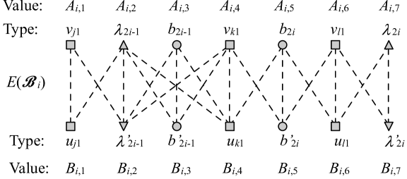
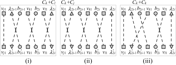
Figure 9: Illustration of reduction.

Figure 10: Three possible transition matchings for $\mathcal{B}_{i}$.

As shown in Figure 10, the nodes on the upper and lower sides in $\mathcal{B}_{i}$ from the left to the right are associated with the following values

$$(A_{i,1},\cdots,A_{i,7})=(\kappa_{i},\kappa_{i}-1,\kappa_{i}-2,\kappa_{i}-2,\kappa_{i}-3,\kappa_{i}-4,\kappa_{i}-5),\mbox{ and}$$ (18)

$$(B_{i,1},\cdots,B_{i,7})=(iK,iK+1,iK+2,iK+2,iK+3,iK+4,iK+5),$$ (19)

respectively, where $\kappa_{i}=(n+1-i)K$ and $K$ is any integer $\geq 7$; $LB=(n+1)K-1$ and $UB=(n+1)K+1$. Each edge in $\mathcal{B}(V,U)$ has weight equal to the sum of the values of its end points.

The instance of 2SLW consists of $7n$ jobs, in which $2n$ jobs associated with pairs of $b$-nodes are $I_{01}=\{(b_{2i-1},b_{2i-1}^{\prime})$, $(b_{2i},b_{2i}^{\prime}):1\leq i\leq n\}$, $3n$ jobs associated with $v$-nodes are $I_{02}=\{(v_{i1},u_{i2})$, $(v_{i2},u_{i3})$, $(v_{i3},u_{i1}):i=1,...,n\}$, and $2n$ jobs associated with pairs of $\lambda$-nodes are $I_{03}=\{(\lambda_{i},\lambda_{i\oplus 1}^{\prime})$, $(\lambda_{i\oplus 1},\lambda_{i\oplus 2}^{\prime}):1\leq i\leq n\}$. Note that $I_{0}=I_{01}\cup I_{02}\cup I_{03}$ is a perfect matching for $\mathcal{B}(V,U)$, and such a matching is called a city matching.

The crux of the remaining construction is based on the idea of relating a permutation of the $7n$ jobs $(J_{[1]},J_{[2]},...,J_{[7n]})$ in the constructed 2SLW instance to a perfect matching in $\mathcal{B}(V,U)$ in such a way that $(W_{[i]2},W_{[(i\ mod\ 7n)+1]1})$, $1\leq i\leq 7n$, are matches. Note that $W_{[i]2},W_{[i+1]1}$ are the two tasks performed by stations $ST1$ and $ST2$, respectively, simultaneously at a certain time. One can easily observe that, because of bounds $LB$ and $UB$, any matching $N$ as a solution for 2SLW cannot involve a edge connecting two different blocks, and the only edges which can be included in $N$ in each block are the dash lines in Figure 10. Such a perfect matching $N$ is called a transition matching. If $I_{0}\cup N$ forms a Hamiltonian cycle for $\mathcal{B}(V,U)$, then it is called complementary Hamiltonian cycle (CHC).

We use notation $(\cdot,\cdot)$ (resp., $[\cdot,\cdot]$) to indicate an edge of a city matching (resp., transition matching). Consider a special transition matching $N_{D}=\{[A_{i,j},B_{i,j}]:i=1,...,n,j=1,...,7\}$. $I_{0}\cup N_{D}$ consists of a master $\lambda$-subcycle $\mathcal{C}_{\lambda}=[\lambda_{1},\lambda_{1}^{\prime}](\lambda_{1}^{\prime},\lambda_{2})...[\lambda_{i},\lambda_{i}^{\prime}](\lambda_{i}^{\prime},\lambda_{i\oplus 1})...[\lambda_{n},\lambda_{n}^{\prime}](\lambda_{n}^{\prime},\lambda_{1})$, $n$ $v$-subcycles $\mathcal{C}_{i}$ for $i=1,...,n$ (e.g., $\mathcal{C}_{1}=[v_{11},u_{11}](u_{11},v_{12})[v_{12},u_{12}](u_{12},v_{13})[v_{13},u_{13}](u_{13},v_{11})$), and $2n$ $b$-subcycles $\mathcal{C}_{b}=[b_{i},b_{i}^{\prime}](b_{i},b_{i}^{\prime})$ for $i=1,...,n$. Hence, a CHC for $\mathcal{B}(V,U)$ is formed by combining the $3n+1$ subcycles. From [13], in order to yield a CHC for $\mathcal{B}(V,U)$, there are exactly three possible transaction matchings for $\mathcal{B}_{i}$ as shown in Figure 10. The design is such that edge $(v_{i},v_{l})$ (resp., $(v_{i},v_{j})$ and $(v_{i},v_{k})$) is in a HC of G if Figure 10(i) (resp., (ii) and (iii)) is the chosen permutation for the constructed 2SLW instance. Following a somewhat complicated argument, [13] proved that there exists a Hamiltonian cycle (HC) for the cubic graph $G$ if and only if there exists a CHC for $\mathcal{B}(V,U)$, and such a CHC for $\mathcal{B}(V,U)$ in turn suggest a sufficient and necessary condition for a solution for 2SLW.

Proofs of Theorem 7. (Sketch) Now we are ready to show the theorem. We only consider the DE4 problem; the DE3 problem is similar and in fact simpler. Recall that the DE4 problem is equivalent to finding a balloon drawing optimizing $optSOP$. Consider the following decision problem:

$\mbox{\sc The DE4 Decision Problem}:$

Given a star graph with flexible uneven angles specified by Equation (3) and an integer $UB$, determine whether a drawing (i.e., specified by the permutation $\sigma\in\Sigma$ and the assignments (0 or 1) for $t_{i}$ ($1\leq i\leq n$)) exists so that $SOP_{\sigma,t}\leq UB$.

It is obvious that the problem is in NP; it remains to show NP-hardness, which is established by a reduction from HC-CG. In spite of the similarity between our reduction and the reduction from HC-CG to 2SLW ([13]) explained earlier, the correctness proof of our reduction is a lot more complicated than the latter, as we shall explain in detail shortly.

In the new setting, Equations (18) and (19) become:

$$(A_{i,1},\cdots,A_{i,7})=(\kappa(i),\kappa(i)-2,\kappa(i)-3,\kappa(i)-4,\kappa(i)-6,\kappa(i)-8,\kappa(i)-9);$$

$$(B_{i,1},\cdots,B_{i,7})=(9ni,9ni+1,9ni+2,9ni+3,9ni+5,9ni+7,9ni+9)$$

for $i=1,2,...,n$ where $\kappa(i)=9n(2n+2-i)$, $n\geq 2$, and $UB=\sum_{i=1}^{7n}M_{i}m_{i}+7n$ where $M_{i}$ (resp., $m_{i}$) is the $i$-th maximum (resp., minimum) among the $14n$ values. (Note that such a setting satisfies the premise of Inequality (8) in Lemma 1, and hence can utilize the inequality.) Hence, we have that:

$$A_{i,j} > B_{i,j},\mbox{ for any $i,j$;}$$

$$A_{i,j} > A_{k,l}\mbox{ and }B_{i,j}<B_{k,l}\mbox{ if ($i<k$) or ($i=k$ and $j<l$).}$$

Note that the above implies that the $j$-th upper (resp., lower) node in $\mathcal{B}_{i}$ is $M_{7i+j}$ (resp., $m_{7i+j}$) for $i\in\{1,...,n\}$ and $j\in\{1,...,7\}$. Define $r_{a,b}=M_{7i+a}-M_{7i+b}$ and $s_{a,b}=m_{7i+a}-m_{7i+b}$ in $\mathcal{B}_{i}$. Hence,

$$r_{1,2}s_{2,1}=2,\ r_{2,3}s_{3,2}=1,\ r_{3,4}s_{4,3}=1,r_{4,5}s_{5,4}=4,\ r_{5,6}s_{6,5}=4,\ r_{6,7}s_{7,6}=2,$$

which are often utilized throughout the remaining proof.

If $\Omega$ is a set of transition edges, the sum of the transition edge weights is denoted by $c(\Omega)$. If $C_{H}=I_{0}\cup N$ is a CHC for $\mathcal{B}(V,U)$ where $I_{0}$ (resp., $N$) is the city matching (resp., transition matching) of the CHC and $t_{i}=0$ for $i=1,...,n$ (i.e., flipping sub-wedges is not allowed), then $c(N)=\sum_{e\in N}c(e)=SOP_{\sigma,t}$ where $c(e)$ is the weight of the transition edge $e$.

Now based on the above setting, we show that there exists a HC for the cubic graph $G$ if and only if there exists a CHC $C_{H}=I_{0}\cup N$ for the instance $\mathcal{B}(V,U)$ of the DE4 problem such that $c(N)\leq UB$.

Suppose that $G$ has a Hamiltonian cycle $C_{H}$. Let $C_{H}=v_{[1]},v_{[2]},...,v_{[n]}$. The construction of a solution for $\mathcal{B}(U,V)$ is the same as [13], as explained in the following. Initiating with $\mathcal{B}_{[1]}$, there exists a pair ($u_{[2]},v_{[2]}$) of nodes in $V\times U$ corresponding to $v_{[2]}\in G$ because $v_{[1]}$ is connected with $v_{[2]}$. From [13], we have that $\mathcal{C}_{\lambda}$ is merged with $\mathcal{C}_{l}$, $\mathcal{C}_{j}$, and $\mathcal{C}_{k}$ respectively in Figure 10 (i), (ii), and (iii). Hence, considering the order of $B_{[1]},B_{[2]},...,B_{[n]}$, in iteration $i$, by choosing the appropriate transition matching, say $N_{[i]}$, of $\mathcal{B}_{i}$ from the three possible matchings in Figure 10, $N_{[i]}$ merges $\mathcal{C}_{[i\oplus 1]}$ with the master subcycle $\mathcal{C}_{\lambda}$. Besides, since the two $b$-subcycles in each $\mathcal{B}_{i}$ also are merged with $\mathcal{C}_{\lambda}$ in any matching of Figure 10, we can obtain a complementary cycle traversing all nodes in $\mathcal{B}(U,V)$.

We need to check $c(N)\leq UB$. In fact, we show that $c(N)=UB$ as follows. It suffices to show that $c(N_{i})=\sum_{j=1}^{7}M_{7i+j}m_{7i+j}+7$ for any $i\in\{1,...,n\}$ where $N_{i}$ is the transition matching for $\mathcal{B}_{i}$. Denote $\Delta c(N_{i})=c(N_{i})-\sum_{j=1}^{7}M_{7i+j}m_{7i+j}$. We can prove that $\Delta c(N_{i})=7$ for every matching in Figure 10. Case (i) is shown as follows, and the others are similar:

$$\Delta c(N_{i}) = M_{7i+1}m_{7i+1}+M_{7i+2}m_{7i+3}+M_{7i+3}m_{7i+2}+M_{7i+4}m_{7i+5}$$

$$+M_{7i+5}m_{7i+4}+M_{7i+6}m_{7i+7}+M_{7i+7}m_{7i+6}-\sum_{j=1}^{7}M_{7i+j}m_{7i+j}$$

$$= r_{2,3}s_{3,2}+r_{4,5}s_{5,4}+r_{6,7}s_{7,6}=1+4+2=7$$

From the above computation, one should notice that if $M_{j}$ is matched with a sub-wedge larger than $m_{j}$ and $M_{j+1}$ is matched with a sub-wedge less than $m_{j+1}$ for $j\in\{7i+1,7i+2,...,7i+6\}$, then $\Delta c(N_{i})$ includes $r_{j,j+1}s_{j+1,j}$.

The converse, i.e., showing the existence of a CHC $C_{H}=I_{0}\cup N$ for the instance $\mathcal{B}(V,U)$ of DE4 with $c(N)\leq UB$ implies the presence of a HC in $G$, is rather complicated. The key relies on the following three claims.

1. (Bipartite) There are no transition edges in $N$ between any pairs of upper (resp., lower) nodes in $C_{H}$.

2. (Block) There are no transition edges in $N$ between two blocks in $C_{H}$.

3. (Matching) There is only one of $\mathcal{C}_{j}$, $\mathcal{C}_{k}$, and $\mathcal{C}_{l}$ merged with the master subcycle $\mathcal{C}_{\lambda}$ in each $\mathcal{B}_{i}$. (Recall that each node $v_{i}$ is adjacent to $v_{j}$, $v_{k}$, $v_{l}$ in $G$, and hence the statement implies the presence of a HC in $G$.)

For proving the above statements, we need the following claims:

Claim 1

(see [5]) Given two transition matchings $N$ and $N^{\prime}$ between $V$ and $U$, there exists a sequence of exchanges which transforms $N$ to $N^{\prime}$.

Claim 2

If $N$ is a transition matching between $V$ and $U$ and involves two edges $e_{1}$ and $e_{2}$ crossing each other, then $c(N)>c(N^{\prime})$ for $N^{\prime}=N\otimes(e_{1},e_{2})$.

(Claim 2 can be proved by easily checking $c(N)-c(N^{\prime})>0$.) It is very important to notice that Claim 2 can be adapted even when $I_{0}\cup N$ may NOT be a CHC. The transition matching where $M_{j}$ is matched with $m_{j}$ for every $j$ (every transition edge is visually vertical) is denoted by $N_{D}$, i.e., $c(N_{D})=\sum_{j=1}^{7n}M_{j}m_{j}$. Note that if each edge in $N$ is between $V$ and $U$, we can obtain $c(N)>c(N_{D})$ by repeatedly using Claim 2 in the order from the leftmost node to the rightmost node of $V$, similar to the technique in the proof of Claim 1 [5].

Proof of Statement (S-1). Supposing that there exits $\overline{k}\geq 1$ transition edges between pairs of upper nodes in $C_{H}$, then there must exist $\overline{k}$ transition edges between pairs of lower nodes in $C_{H}$, by Pigeonhole Principle. Select one of the upper (resp., lower) transition edges, say $e_{1}=(M_{a},M_{b})$, (resp., say $e_{2}=(m_{p},m_{q})$). Consider $N^{\prime}=N\otimes(e_{1},e_{2})$. Then $c(N)-c(N^{\prime})=(M_{a}-m_{p})(M_{b}-m_{q})\geq(M_{n}-m_{n})^{2}=18^{2}(n-1)^{2}>7n$. Hence, $c(N)>c(N^{\prime})+7n$. By the same technique, we can find $N^{\prime\prime}$ where each edge in $N^{\prime\prime}$ is between $U$ and $V$ such that $c(N)>c(N^{\prime\prime})+7\overline{k}n\geq c(N^{\prime\prime})+7n\geq c(N_{D})+7n=UB$, which is impossible.

Proof of Statement (S-2). By Statement (S-1), each edge in the transition matching of $C_{H}$ is between $V$ and $U$. Suppose there exists at least one transition edge between two blocks. Assume there are $l$ blocks, $\{\mathcal{B}_{k_{1}},\mathcal{B}_{k_{2}},...,\mathcal{B}_{k_{l}}\}$, with transition edges across two blocks. Let $k_{min}=\min(k_{1},k_{2},...,k_{l})$. Consider $e_{1}=(M_{a},m_{d})$ is the transition edge between $\mathcal{B}_{k_{min}}$ and $\mathcal{B}_{k_{i}}$ for $i\in\{1,...,l\}$, and $k_{min}\neq k_{i}$. Then there must exist a transition edge connecting to one of the lower nodes of $\mathcal{B}_{k_{min}}$, say $m_{c}$, by Pigeonhole Principle, and we say the edge $e_{2}=(M_{b},m_{c})$ where $m_{c}$ and $M_{b}$ are respectively from $\mathcal{B}_{k_{min}}$ and $\mathcal{B}_{k_{j}}$ for $j\in\{1,...,l\}$ and $k_{j}\neq k_{min}$. Note that $e_{2}$ must cross $e_{1}$ because $M_{a}$ and $m_{c}$ are in $\mathcal{B}_{k_{min}}$, i.e., $M_{a}>M_{b}$ and $m_{c}<m_{d}$. Besides, we have $M_{a}\geq M_{b}+9n-9$ and $m_{d}\geq m_{c}+9n-9$ because two end points of edge belong to different blocks. Consider $N^{\prime}=N\otimes(e_{1},e_{2})$. Then $c(N)-c(N^{\prime})=(M_{a}-M_{b})(m_{d}-m_{c})\geq(9n-9)^{2}>7n$ for $n\geq 2$. That is, $c(N)>c(N^{\prime})+7n\geq c(N_{D})+7n$, which is a contradiction.

Proof of Statement (S-3). Recall that $I_{0}\cup N_{D}$ in every $\mathcal{B}_{i}$ involves subcycles $\mathcal{C}_{j}$, $\mathcal{C}_{\lambda}$, $\mathcal{C}_{b_{2i-1}}$, $\mathcal{C}_{k}$, $\mathcal{C}_{b_{2i}}$, $\mathcal{C}_{l}$, $\mathcal{C}_{\lambda}$ from the leftmost to the rightmost. If there exists a CHC $C_{H}=I_{0}\cup N$ for the instance $\mathcal{B}(V,U)$, each $b$-subcycle in $\mathcal{B}_{i}$ has to be merged with some subcycle in the same $\mathcal{B}_{i}$ by Statements (S-1) and (S-2). $\Delta c(N_{i})$ is at least 5 due to the merging of $b$-subcycles from the following four cases (here it suffice to discuss the merging of $b$-subcycles with their adjacent subcycles because $\Delta c(N_{i})$ in others cases are larger):

1. $\mathcal{C}_{b_{2i-1}}$ merged with $\mathcal{C}_{\lambda}$ and $\mathcal{C}_{b_{2i}}$ merged with $\mathcal{C}_{k}$: $\Delta c(N_{i})>r_{2,3}s_{3,2}+r_{4,5}s_{5,4}=1+4=5$

2. $\mathcal{C}_{b_{2i-1}}$ merged with $\mathcal{C}_{\lambda}$ and $\mathcal{C}_{b_{2i}}$ merged with $\mathcal{C}_{l}$: $\Delta c(N_{i})>r_{2,3}s_{3,2}+r_{5,6}s_{6,5}=1+4=5$

3. $\mathcal{C}_{b_{2i-1}}$ merged with $\mathcal{C}_{k}$ and $\mathcal{C}_{b_{2i}}$ merged with $\mathcal{C}_{k}$: $\Delta c(N_{i})>r_{3,4}s_{4,3}+r_{4,5}s_{5,4}=1+4=5$

4. $\mathcal{C}_{b_{2i-1}}$ merged with $\mathcal{C}_{k}$ and $\mathcal{C}_{b_{2i}}$ merged with $\mathcal{C}_{l}$: $\Delta c(N_{i})>r_{3,4}s_{4,3}+r_{5,6}s_{6,5}=1+4=5$

Recall that there are $3n+1$ subcycles in $\mathcal{B}$. Hence we require at least $3n$ times of merging subcycles to ensure these subcycles to be merged as a CHC. Since we have discussed that two $b$-subcycles have to be merged in each $\mathcal{B}_{i}$ (i.e., the total times of merging $b$-subcycles are $2n$), we require at least $n$ more times of merging subcycles to obtain a CHC. In fact, the $n$ times of merging subcycles is because each $\mathcal{B}_{i}$ contributes once of merging subcycles. As a result, Statement (S-3) is proved if we can show that after merging two $b$-subcycles in each $\mathcal{B}_{i}$, the third merging subcycles in $\mathcal{B}_{i}$ is to merge one of $C_{j}$, $C_{k}$, and $C_{l}$ with $C_{\lambda}$.

In what follows, we discuss $\Delta c(N_{i})$ when there are exactly $\overline{h}$ times of merging subcycles in $N_{i}$:

• If $\overline{h}=2$, then $\Delta c(N_{i})>5$.

• If $\overline{h}=3$ and the transition matching of $\mathcal{B}_{i}$ is one of the matchings in Figure 10, then $\Delta c(N_{i})=7$.

• If $\overline{h}=3$ and the transition matching of $\mathcal{B}_{i}$ is NOT any of the matchings in Figure 10, then $\Delta c(N_{i})>7$.

• If $\overline{h}=4$, then $\Delta c(N_{i})>9$.

• If $\overline{h}=5$, then $\Delta c(N_{i})>11$.

• If $\overline{h}=6$, then $\Delta c(N_{i})>13$.

If the above statements on $\overline{h}$ hold, then Statement (S-3) hold. The reason is as follows. Remind that we need $3n$ times of merging subcycles to be a CHC. Therefore, if there exists a transition matching of $\mathcal{B}_{i}$ with $\overline{h}=2$ for some $i$ (i.e., there are exactly two times of merging subcycles in $\mathcal{B}_{i}$), then there must exists a $\mathcal{B}_{j}$ for some $j$ with $\overline{h}\geq 4$. Then $\Delta c(N_{i})+\Delta c(N_{j})>14$, which is impossible because this results in the total $\Delta c$ larger than $7n$.

Proof of Statements on $\overline{h}$. Note that the transition matching of every $\mathcal{B}_{i}$ can be viewed as a permutation of $\{M_{7i+1},M_{7i+2},...,M_{7i+7}\}$ (a mapping from $V$ to $U$), and hence different ordering or different times of merging subcycles lead to a permutation with different factors, e.g, the permutation for Figure 10(i) is $\langle M_{7i+1}\rangle\langle M_{7i+2}M_{7i+3}\rangle\langle M_{7i+4}M_{7i+5}\rangle\langle M_{7i+6}M_{7i+7}\rangle$. If we let $f=\langle M_{j_{1}},M_{j_{2}},...,M_{j_{h}}\rangle$ be a nontrivial factor of the permutation for $N_{i}$, then $c(N_{i})\geq c(f)\geq\sum_{k=j_{1}}^{j_{h}}M_{k}m_{k}+\sum_{k=j_{1}}^{j_{h-1}}r_{k,k+1}s_{k+1,k}$ by Equation (7) in Lemma 1. Here we concern the value $\sum_{k=j_{1}}^{j_{h-1}}r_{k,k+1}s_{k+1,k}$ induced by $f$ (which is denoted by $\Theta(f)$) because it can be viewed as a lower bound of $\Delta c(N_{i})$.

If a factor $f$ includes $M_{j}$ but excludes $M_{j+1}$, then we say that $f$ has a lack at $M_{j+1}$. We observe that if the permutation $p_{i}$ for $\mathcal{B}_{i}$ has a lack, then we can find a permutation $p_{i}^{\prime}$ for $\mathcal{B}_{i}$ consisting of the factors without any lacks such that $\Theta(p_{i}^{\prime})<\Theta(p_{i})$ in which the number of factors of $p_{i}^{\prime}$ is the same as that of $p_{i}$ and the size of each factor is also the same. The reason is as follows. Assume that $p_{i}$ has a factor $f=\langle...,M_{j},M_{l},...\rangle$ with a lack at $M_{j+1}$ (i.e., $l\neq j+1$) and the minimum number appearing in the factor is $M_{q}$. Let $p_{i}^{\prime}$ be almost the same as $p_{i}$ except the factor $f$ in $p_{i}$ is modified as a factor without any lacks involving $M_{j+1}$ but excluding $M_{q}$ in $p_{i}^{\prime}$. Then by Equation (7) in Lemma 1, $\Theta(p_{i})-\Theta(p_{i}^{\prime})\geq(r_{j,j+2}s_{j+2,j}-r_{j,j+1}s_{j+1,j}-r_{j+1,j+2}s_{j+2,j+1})+r_{q-1,q}s_{q,q-1}\geq 2+1>0$. In the similar way, we can find a permutation with factors without any lacks.

In light of the above, it suffices to consider the permutation for $\mathcal{B}_{i}$ consisting of the factors without any lacks when discussing the lower bound of $c(N_{i})$. Thus, in the following, when we say that the permutation for $\mathcal{B}_{i}$ has a factor $f$, this implies that $f$ has no lacks, so Lemma 1 can be applied to $f$.

Now we are ready to prove the statements on $\overline{h}$. The statement of $\overline{h}=2$ holds because $c(N_{i})$ is increased by at least 5 when two $b$-subcycles have to be merged in each $\mathcal{B}_{i}$. As for the statement of $\overline{h}=6$, note that merging six subcycles implies a permutation with a factor of size seven. Thus, by Equation (7) in Lemma 1, $\Delta c(N_{i})\geq\sum_{j=1}^{6}r_{j,j+1}s_{j+1,j}=2+1+1+4+4+2=14>13$, as required. Let $\psi=\sum_{j=1}^{6}r_{j,j+1}s_{j+1,j}=14$ for the convenience of the following discussion. As for the statement of $\overline{h}=5$, the permutation involves two nontrivial factors after five times of merging subcycles. Note that one of the two factors has size at least four, and hence the factor $\langle j_{1},...,j_{4}\rangle$ contributes $\sum_{k=j_{1}}^{j_{4}}M_{k}m_{k}+\sum_{k=j_{1}}^{j_{4}}r_{k,k+1}s_{k+1,k}+(4-2)$ by Equation (8) in Lemma 1. Therefore, by Equation (7) in Lemma 1, $\Delta c(N_{i})\geq\psi-r_{x,x+1}s_{x+1,x}+(4-2)=16-r_{x,x+1}s_{x+1,x}$ for some $x\in\{1,...,6\}$. (Note that $-r_{x,x+1}s_{x+1,x}$ suggests that $M_{x}$ and $M_{x+1}$ are in different factors.) Since $r_{x,x+1}s_{x+1,x}\leq 4$, hence $\Delta c(N_{i})\geq 12>11$, as required.

As for the statement of $\overline{h}=4$, by Equation (7), $\Delta c(N_{i})\geq\psi-r_{x,x+1}s_{x+1,x}-r_{y,y+1}s_{y+1,y}$ for some $x,y\in\{1,...,6\}$ and $x\neq y$. Discuss all possible cases of pair $(x,y)$ as follows. Consider one of $x,y$ is 2 or 3. We assume that $x=2$, and the other case is similar. Hence, $r_{x,x+1}s_{x+1,x}=1$. Since $r_{y,y+1}s_{y+1,y}\leq 4$ and there exists a factor with size at least three in this case, $\Delta c(N_{i})\geq\psi-1-4+(3-2)=10>9$ by Equation (8), as required. The remaining cases are $(1,4),(1,5),(1,6),(4,5),(4,6)$, and $(5,6)$. Consider one of $x,y$ is 1 or 6. We assume that $x=1$, and the other case is similar. Hence $r_{x,x+1}s_{x+1,x}=2$. Since $r_{y,y+1}s_{y+1,y}\leq 4$ and there exists a factor with size at least four or two factors with size at least three in this case, $\Delta c(N_{i})\geq\psi-2-4+(4-2)\vee 2(3-2)=10>9$ by Equation (8), as required. Last, consider $(x,y)=(4,5)$, namely, $M_{4}$ and $M_{5}$ (resp., $M_{5}$ and $M_{6}$) are in different factors. Hence, $M_{5}$ cannot be matched with $m_{4}$ nor $m_{6}$, i.e., subcycle $\mathcal{C}_{b_{2i}}$ cannot be merged with adjacent subcycles $\mathcal{C}_{k}$, $\mathcal{C}_{l}$. Since merging $\mathcal{C}_{b_{2i}}$ with $\mathcal{C}_{b_{2i-1}}$ induces the smallest cost $r_{3,5}s_{53}=9$ in this case, and the other two times of merging subcycles must induce cost more than 2, hence $\Delta c(N_{i})$ is at least 9.

As for the two statements of $\overline{h}=3$, by Equation (Appendix), $\Delta c(N_{i})$ in the case when $N_{i}$ is one of the matchings in Figure 10 is exactly seven, as required. Then we consider the case when $N_{i}$ is not in Figure 10 in the following. By Equation (7), $\Delta c(N_{i})\geq r_{x,x+1}s_{x+1,x}+r_{y,y+1}s_{y+1,y}+r_{z,z+1}s_{z+1,z}\geq 5+r_{z,z+1}s_{z+1,z}$ for some $x,y,z\in\{1,...,6\}$ and $x\neq y\neq z\neq x$ since it is necessary to merge $b$-subcycles, which contributes at least 5. It suffices to consider the cases when $r_{z,z+1}s_{z+1,z}\leq 2$, which may violate our required. That is, $z$ may be 1, 2, 3 or 6. By considering four possible cases of merging $b$-subcycles, one may easily check that whatever $z$ is, $\Delta c(N_{i})$ must be either larger than 7 or in Figure 10.

References

- [1] G. D. Battista, P. Eades, R. Tammassia, I. G. Tollis, Graph Drawing: Algorithms for the Visualization of Graphs, Prentice Hall, 1999.
- [2] J. Carrire, R. Kazman, Research report: Interacting with huge hierarchies: Beyond cone trees, in: IV 95, IEEE CS Press, 1995.
- [3] P. Eades, Drawing free trees, Bulletin of Institute for Combinatorics and its Applications (1992) 10–36.
- [4] C. Jeong, A. Pang, Reconfigurable disc trees for visualizing large hierarchical information space, in: InfoVis ’98, IEEE CS Press, 1998.
- [5] M.-Y. Kao, M. Sanghi, An approximation algorithm for a bottleneck traveling salesman problem, Journal of Discrete Algorithms 7 (3) (2009) 315–326.
- [6] K. Kaufmann, D. Wagner (Eds.), Drawing Graphs: Methods and Models, vol. 2025 of LNCS, Springer, 2001.
- [7] H. Koike, H. Yoshihara, Fractal approaches for visualizing huge hierarchies, in: VL ’93, IEEE CS Press, 1993.
- [8] C.-Y. Lee, G. L. Vairaktarakis, Workforce planning in mixed model assembly systems, Operations Research 45 (4) (1997) 553–567.
- [9] C.-C. Lin, H.-C. Yen, On balloon drawings of rooted trees, Journal of Graph Algorithms and Applications 11 (2) (2007) 431–452.
- [10] G. Melançon, I. Herman, Circular drawing of rooted trees, Reports of the Centre for Mathematics and Computer Sciences, Report number INS-9817.
- [11] E. Reingold, J. Tilford, Tidier drawing of trees, IEEE Trans. Software Eng. SE-7 (2) (1981) 223–228.
- [12] Y. Shiloach, Arrangements of planar graphs on the planar lattice, Ph.D. thesis, Weizmann Institute of Science (1976).
- [13] G. L. Vairaktarakis, On Gilmore-Gomory’s open question for the bottleneck TSP, Operations Research Letters 31 (6) (2003) 483–391.