Preheating in Bubble Collisions

Abstract

In a landscape with metastable minima, the bubbles will inevitably nucleate. We show that during the bubbles collide, due to the dramatically oscillating of the field at the collision region, the energy deposited in the bubble walls can be efficiently released by the explosive production of the particles. In this sense, the collision of bubbles is actually highly inelastic. The cosmological implications of this result are discussed.

When the universe is initially set in a metastable minimum of certain landscape of scalar fields, it will undergo a dS expansion, bubbles with lower energy minima will inevitably nucleate in this background [1]. When the radius of bubble is larger than its critical radius, the bubble will expand outwards, and eventually collide with other expanding bubbles. In general, it is expected that during the bubbles collide, the energy deposited in the bubble walls will be released, e.g.[2]. This release of energy is significant, e.g. in old inflation [3], extended inflation [4], and [5],[6],[7],[8], the universe is reheated by it.

The bubble collision has been studied earlier in [9],[10]. In general, when the bubbles collide, the walls of bubbles will pass through each other or be reflected. The region between outgoing walls remains in high energy metastable minimum, while other region is not affected. However, there is a net force, which will compel the walls to rest, and then back and move towards each other. Thus the collision of walls will inevitably occur again and again. This oscillation of walls has be displayed in the numerical simulations for bubble collision [9],[11],[12],[13]. In general, it is thought that during the bubble collision the energy deposited in the walls will be released by the direct decaying of scalar wave into other particles, e.g.[11],[14], or the gravitational radiation, e.g.[12],[15],[16],[17]. However, this release of the energy might be more dramatic than expected. In this paper, we show that due to the oscillation of the background field at the collision region, the energy can be efficiently released by the explosive production of the particles.

We begin with a brief review of the numerically simulation of the collision of bubbles nucleating in a given potential in Fig.1, in which the high energy metastable minimum is $\phi_{F}$ and the low energy minimum is $\phi_{T}$. We only care the numerical results of the evolution of field at the collision region during the bubble collision. Thus the details of the equations of the nucleation and evolution of bubble are neglected, see e.g.[18],[19].

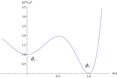
Figure 1: The potential with two minima, which will be used in the numerical simulations of the bubble collision in Figs.2 and 4, and the production of $\chi$-particle in collision region in Fig.3. $\eta\equiv|\phi_{T}-\phi_{F}|$ is a normalized parameter with mass dimension. The parameter we used is $\eta=0.01$ for whole paper.

The field $\phi$ is initially in $\phi_{F}$. Thus the universe is inflating. Then the bubbles with $\phi_{T}$ will be expected to nucleate. The radius of bubble is determined by the instanton equation of $\phi$. We have numerically solved this instanton equation and will use the data obtained as the initial state of bubbles which will collide. Their initial distance is defined as $D_{0}$. Here we choose $D_{0}\sim{375\over\eta}<{1\over H_{F}}$, where $H_{F}$ is the Hubble rate of the false vaccum which can be estimated by $H_{F}\simeq\sqrt{V(\phi_{F})}/M_{P}$ and in this paper $H_{F}\simeq\eta^{2}/100$. $M_{P}=1$ is set for whole paper and $\eta$ is the normalized parameter with mass dimension, see Fig.1. The nucleation radius of the bubbles is $R_{0}={3\sigma/V_{F}}$, which can be given by

$$R_{0}=\frac{3\int^{\phi_{T}}_{\phi_{F}}\sqrt{2V\left(\phi\right)}d\phi}{V_{F}}\sim 0.3\frac{3\sqrt{2}\eta}{\sqrt{V_{F}}},$$ (1)

where $\sigma$ is the surface tension of bubble wall, which means that $H_{F}R_{0}\sim 3\sqrt{2}\eta\ll 1$, since $\eta\ll 1$ and in the simulations $\eta=0.01$ is actually used.

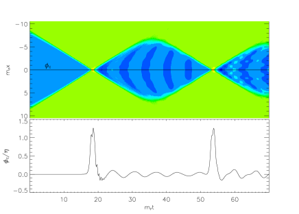
Figure 2: The numerical simulation of bubbles collision. The color panel describes the evolution and collision of bubbles after their nucleations, where the green region denotes the region in $\phi_{T}$ while the blue region denotes that in $\phi_{F}$, and the light blue region between them denotes the bubble wall. We can see that during the bubbles collision the bubble walls will be oscillating around the center of bubbles collision, which induces that at the collision region the field $\phi$ initially in $\phi_{F}$ overshoots to $\phi_{T}$ and then backs to $\phi_{F}$, and oscillates around $\phi_{F}$. The lower panel is that of $\phi_{C}$ in color panel. Here $M_{F}\sim 0.04\eta$.

In the simulation of the evolution and collision of bubbles, we will neglect the gravitational effect, which is not important since $V(\phi)\ll 1$, the nucleation radius of bubbles $R_{0}H_{F}\ll 1$, their initial separation $D_{0}H_{F}\ll 1$ and the time per oscillation, which can be found in Fig.2, $50/M_{F}\simeq 125/\eta\ll 1/H_{F}$ . We solve the evolving equation $\square\phi=\partial_{\phi}V$ of field with the flat space metric in 3+1D by using a modified version of LatticeEasy [20] and 2048 lattices, in which the initial data of bubbles is given by the instanton equation, and at $t=0$, $x=\pm 0.5{D_{0}}$ is considered, since the collided bubbles can be boosted into a particular frame in which they are nucleated at the same time. The program is ran with double precision. The time step is small enough to guarantee the Courant stability condition. In the meantime, we checked the results by using higher precision, and found that the results are same. The numerical result is plotted in Fig.2, in which the width in space is actually far larger than that in time, and the most of regions irrelevant with the bubbles collision is cut out to make the colliding region in figure clearer.

The color panel in Fig.2 is that of the evolution and collision of bubbles in position space. We define the value of $\phi$ field in a small region around the collision center as $\phi_{C}$. The lower panel of Fig.2 is the evolution of $\phi_{C}$, which can be explained as follows. $\phi_{C}$ before collision rests with $\phi_{C}=\phi_{F}$. However, when the collide occurs, the gradient energy of this region will become large, which will induce $\phi_{C}$ get cross the potential barrier, overshoot $\phi_{T}$. Then it backs to $\phi_{F}$ and oscillates. This behavior is repeated during the following collisions of bubble walls. However, when there is the third lower energy minimum $\phi_{3}$, after overshooting $\phi_{T}$, the field at the collision region might not back to $\phi_{F}$, and straightly run into $\phi_{3}$. Thus a new bubbles will be generated [21].

We introduce a coupling of the background field $\phi$ with $\chi$ as follows

$$\mathcal{L}_{int}=-\frac{1}{2}g^{2}(\phi-\phi_{*})^{2}\chi^{2},$$ (2)

where $g$ is the coupling constant, and $\phi_{*}$ is a parameter between $0$ and $1$, see the renormalization in Fig.1.

We will neglect the expansion of space. However, the result is not altered qualitatively by the inclusion of expansion. The evolution of $\phi$ at the collision region is given by $\phi_{C}$ in Fig.2. This coupling means that when $|\phi_{C}-\phi_{*}|\sim 0$, the adiabatic condition becomes violated, the parametric resonance will inevitably occur, which will result in the explosive production of $\chi$-particles at corresponding region, similar to the preheating after inflation [22],[23], which has been intensively studied, e.g.[24],[25].

The initial width $d_{0}$ of bubble wall can be estimated as $d_{0}\sim\frac{3}{2}{\eta\over\sqrt{V_{bar}}}$ [9], in which $V_{bar}$ is the effective height of the potential barrier. This width will become $d=d_{0}/\gamma$ at the time of bubbles collision, in which $\gamma$ can be given by $\gamma={D_{0}\over 2R_{0}}+1$, where it is noticed that $D_{0}$ is the distance between the bubble walls at the time of their nucleations. When the parameters in Fig.1 are considered, $d_{0}\sim 132/\eta$ and $\gamma\sim 2.5$ are obtained. Thus $d\simeq 53/\eta$. Then, in the linear order the velocity that $\phi_{C}$ passes through $\phi_{*}$ can be estimated as $\dot{\phi}_{*}\simeq\Phi_{C}/d$. Thus in a very short interval $\Delta t\sim 1/\sqrt{g{\dot{\phi}}_{*}}\simeq\sqrt{\frac{\gamma}{gd_{0}\Phi_{C}}}~{}d$, the adiabatic condition is broken. Thus the characteristic momentum is given by

$$k_{*}\sim(\Delta t)^{-1}\simeq\sqrt{g{\dot{\phi}}_{*}}\simeq\sqrt{g\Phi_{C}\over d},$$ (3)

which means $\Delta t\sim 0.35d$ and $k_{*}\sim 3/d$. This is consistent with general assumption that the energy of particles produced by the bubbles collision is about $\sim 1/d$, e.g.[14].

During the bubbles collide, the collision of the bubble walls is periodical, which induces $|\phi_{C}-\phi_{*}|\sim 0$ twice at each time of the collisions of bubble walls, since $\phi_{C}$ overshoots to $\phi_{T}$ and then backs to $\phi_{F}$. During $\Delta t$ in each time, $\phi_{C}(t)$ can be regarded as $\phi_{C}(t)\simeq{\dot{\phi}}_{*}\left(t-t_{*}\right)$. Thus the motion equation of mode ${X}_{k}$ of $\chi$ during $\Delta t$ is given by

$$\frac{d^{2}{X}_{k}}{dt^{2}}+\left(k^{2}+{g^{2}\Phi_{C}^{2}\over d^{2}}(t-t_{*})^{2}\right){X}_{k}=0,$$ (4)

which gives the evolution of ${X}_{k}$, and thus $n_{k}$ after each collision of bubble walls. Thus the occupation number $n_{\chi_{k}}$ of $X_{k}$ mode after the $N$th collision of bubble walls, in large $n_{k}^{i}$ limit, is given by $n_{\chi_{k}}\sim e^{2\pi\sum\limits_{i=1}^{2N}\mu_{k}^{i}}$, where $i$ labels the times that $\phi_{C}$ passes through $\phi_{*}$ and $\mu_{k}^{i}$ is the function of $k/k_{*}=k/\sqrt{g\Phi_{C}/d}$ given in [22]. The number density of $\chi$-particles after the $N$th collision can obtained by integrating $n_{\chi_{k}}$ for $k$, which is

$$n_{\chi}=\frac{1}{8\pi^{3}}\int d^{3}k~{}n_{\chi_{k}}\sim\frac{1}{64\pi^{3}}\left(\frac{g\Phi_{C}}{d}\right)^{3/2}\frac{e^{2\pi\sum\limits_{i=1}^{2N}\mu_{k}^{i}}}{\sqrt{f}},$$ (5)

which has been evaluated by the steepest descent method, where $f=\sum\limits_{i=1}^{2N}\mu^{i}$, $\mu^{i}$ is the maximum of $\mu_{k_{m}}^{i}(k)$, which can be estimated in $k_{m}\sim\sqrt{\frac{g\Phi_{C}}{4d}}$.

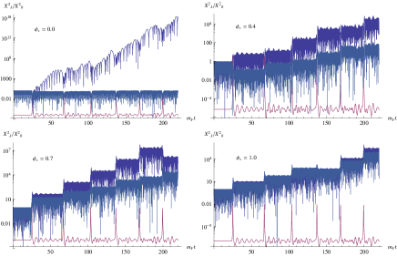
Figure 3: The numerical simulation of the evolution of $X_{k}$ at the collision region for the coupling (2). $\eta=0.01$, $g^{2}=0.5$, and the modes shown are $k=0$ and $k=0.1\eta$, respectively. We also show the evolution of $\phi_{C}$ in red lines.

We calculate the evolution of ${X}_{k}$ numerically in Fig.3 for different values of $\phi_{*}$ by using the data of the bubbles collision in Fig.3. The red lines in this figure denote the evolution of $\phi_{C}$ during the bubbles collision. When the bubble walls collide, the red line has a sharp peak which shows the rapid change of $\phi_{C}$ overshooting to $\phi_{T}$ then backing to $\phi_{F}$ at the time of each collision. Here the backreaction from particle production is not taken into account. However, since during the collisions a little of energy of the walls will transfer into the energy of oscillation of the false vacuum, the speed of the walls decrease after each collision and this will made the peaks of $\Phi_{C}$ drop slightly.

In general, the explosive production of particles induced by the parameter resonance will occur for most $\phi_{*}$ between 0 and 1. However, the resonant behavior are different for different $\phi_{*}$. The intensity of the parametric resonance is depended on the speed of $\phi_{C}$ passes through $\phi_{*}$. The larger the speed is, the more likely the broad resonance is to take place. We can introduce a critical point $\phi_{cri}$ which $\simeq 0.1$ in our simulation. When $\phi_{*}\lesssim\phi_{cri}$, the speed of $\phi_{C}$ is too small for the broad resonance to take place, and only narrow resonance occurs, i.e.$X_{k}$ only increase exponentially in a band of $k$ with narrow width, see in left upper panel of Fig.3, in which $X_{k}$ increases for $k=0$ but is not changed for $k=0.1\eta$, which is similar to the case in [26]. This case is not efficient for the release of energy. When $\phi_{*}>\phi_{cri}$, as given in other panels of Fig.3, the speed of $\phi_{C}$ become larger, the resonance will be broad, i.e. it occurs for any values of $k$. It can be found that for the broad resonance ${X}_{k}$ is only amplified at the time of each collision. In this case, the release of energy can be quite efficient [22].

The energy density of $\chi$-particles produced after the $N$th collision is $\rho_{\chi}=n_{\chi}M_{\chi}$, where $M_{\chi}\sim k_{*}\simeq\sqrt{g\Phi_{C}/d}$ can be considered. When the energy deposited in the bubble walls is completely released, $\rho_{\chi}$ should be approximately equal to the energy of the corresponding bubble walls in the collision region. Thus this requires

$$n_{\chi}\sqrt{g\Phi_{C}\over d}\sim\gamma{\sigma\over l},$$ (6)

where $R_{0}$ and the surface tension $\sigma$ are given in Eq.(1), $\gamma$ has been mentioned, $l$ describes the effective width of collision region, which is generally $l\simeq 2d$. Thus substituting Eq.(5) into Eq.(6), $N$ can be estimated as

$$N\sim{1\over 4\pi\mu}\ln{\left({64\pi^{3}\sqrt{V_{F}}\gamma\eta\over l{g^{2}\Phi_{C}^{2}}}\right)},$$ (7)

where all $\mu^{i}\simeq\mu$ are adopted. Eq.(7) means the inelastic degree of the bubbles collision is dependent on the coupling $g$ and the parameters of bubbles at the time of collision, which is expected. The larger $g$ is, the larger the inelastic degree is. When the potential given in Fig.1 is introduced, for $g^{2}\simeq 0.5$ used in Fig.3, at least $N\simeq 6$ is required for the complete release of the energy of bubble walls.

It can be significantly noticed that $N$ given by (7) is insensitive to the concrete value of $\phi_{*}$. The reason is that the release of energy is proportional to the velocity of $\phi_{C}$ passing through $\phi_{*}$, which is about $\sqrt{\Phi_{C}/d}$ irrelative with $\phi_{*}$. The simulation of the evolution of field value at the collision region, in which the loss of walls energy is considered, is interesting to grasp the physics of the collision of bubbles. We used the same initial data and parameters with that in Fig.2, and $\phi_{*}=0.4$ without loosing generalization, to perform it in Fig.4. This performance is explained as follows.

Theoretically, when $\phi$ passes through $\phi_{*}$, the preheating leaded by the coupling at $\phi_{*}$ will make the kinetic energy of $\phi$ decreasing, and the loss of energy is proportion to the velocity of $\phi$ at this time. To simulate this effect, we multiplys a factor $1-\beta^{2}<1$ on ${\dot{\phi}}^{2}$ in the corresponding program when $\phi$ pass through $\phi_{*}$ each time. $\beta$ can be calculated by letting the loss of kinetic energy of $\phi$ around $\phi_{*}$ equal to the energy of particles produced at this time, which is given by $\beta\simeq{\sqrt{2n^{i}_{\chi_{k}}M_{\chi}}/{\dot{\phi}_{C}}}$, where $n^{i}_{\chi_{k}}$ denotes the number density of $\chi$-particles produced at each time when $\phi_{C}\simeq\phi_{*}$. In actually simulation, this process is carried out by the cumulation of the time steps around $\phi_{*}$. We can see that after about $N=4$, the blue region denoting $\phi_{F}$ disappears, $\phi_{C}$ at the collision region will oscillate around $\phi_{T}$. The reason is that with the gradual release of the energy in the bubble walls, the oscillation of bubble walls will have smaller and smaller amplitude, which will lead that during the $N$th collision, instead of backing to $\phi_{F}$ during previous collision of walls, after getting cross the potential barrier, $\phi_{C}$ will oscillate around $\phi_{T}$.

In above estimate, the backreaction of $\chi$-particles produced to the evolution of $\phi$ at the collision region has been neglected. However, with the increase of $\chi$-particles, its backreaction will be enhanced gradually, which will inevitably shut off the resonance at certain time or after some collisions of bubble walls. The correction induced by the $\chi$-particles to the potential at the point of $\phi_{C}\simeq\phi_{*}$ is $\Delta M_{*}^{2}\simeq g^{2}<\chi^{2}>$ [22], in which the expectation value of $\chi^{2}$ is given by $<\chi^{2}>\simeq{n_{\chi}/g(\phi_{C}-\phi_{*})}\sim{n_{\chi}/g\Phi_{C}}$. The condition that the backreaction becomes important is $\Delta M^{2}_{*}\simeq V_{*}^{\prime\prime}$, which gives $n_{\chi}\sim V_{*}^{\prime\prime}\Phi_{C}/g$. Thus substituting Eq.(5), we can obtain

$$N_{backreaction}\simeq{1\over 4\pi\mu}\ln{\left({64\pi^{3}V_{*}^{\prime\prime}\sqrt{d^{3}}\over\sqrt{g^{5}\Phi_{C}}}\right)},$$ (8)

which is $N_{backreaction}\simeq 4$ for the parameters in Fig.1 and $g^{2}=0.5$. Thus the backreaction is important only after $N=4$. As displayed in Fig.4, after $N=4$, the metastable $\phi_{F}$ region has basically disappears, $\phi_{C}$ at the collision region will oscillate around $\phi_{T}$. Thus the simulation in Fig.4 without the backreaction is robust.

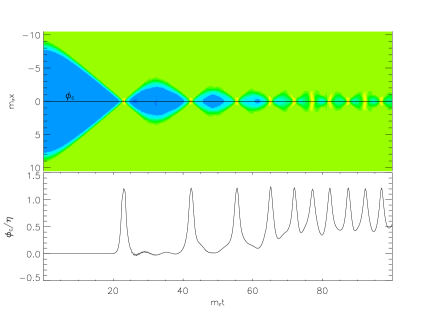
Figure 4: The numerical simulation of bubble collisions, in which the release of walls energy induced by the production of particles at the time of each collision of bubble walls is included, $\phi_{*}=0.4$. The color panel describes the oscillation of bubble walls during the bubble collision. What the green region, the blue region and the light blue region denote are same as that in Fig.2. The lower panel is that of $\phi_{C}$ in color panel.

When $\phi_{C}$ oscillates around $\phi_{T}$, the residual energy is only that of field oscillation, which will be diluted gradually by the expansion of space. However, if $\phi_{*}\simeq 1$, the narrow resonance around $\phi_{T}$ will occur during a following short period, and the residual oscillating energy will continue to be released into the particles. In a word, eventually $\phi_{C}$, i.e.the collision region, will stay at $\phi_{T}$. The collision of bubbles ends.

In conclusion, we have proposed a new possibility of the release of energy deposited in the bubble walls during bubble collisions, not noticed before. When the bubbles collide, the conventionally viewpoint is that the energy in the walls is released by the scalar or gravitational radiation. However, this is not quite efficient. We show that the energy can be efficiently released by the explosive production of the particles, due to the parameter resonance. In this case, the energy in the bubble walls can be drained rapidly. In the example given, the time that the energy is completely released is $60/M_{F}\ll 1/H_{F}$, and the collision times $N=4$ is smaller than $N>13$ when the preheating is not taken into account which is usual expected.

This result has interesting applications in extended inflation and other relevant inflation models, e.g.[6]. It not only helps to obtain the enough reheating temperature in these models, but enrich the phenomenological studies on the reheating of these models. In principle, the preheating in these models could be nearly similar to that in slow roll inflation models. Here, however, the results are dependent on the parameters of bubbles at the time of collision, which are mainly determined by the structure of potential landscape. Thus the preheating in these models could have different predictions from those in slow roll inflation models.

In this paper, we only consider a simple model. In general, dependent on the parameters of bubbles at the time of collision, the oscillation of field at the collision region can be different. However, as long as the coupling of background field $\phi$ to a light scalar field $\chi$ is considered, the explosive production of the particles at the region of bubbles collision will be general. In a landscape with multiple dimensions, such couplings can be actually expected, see [29, 30] for the studies of cosmological models in such a landscape. This means that the collision of bubbles is generally highly inelastic. In principle, the classical $\chi$-wave might be also important for such a coupling. We left the detailed studies and the discussion on its correlation with the $\chi$-particles produced, and the production of particles induced by the collision of bubbles in different potential landscapes in coming works.

The production of particles makes the bubble collision highly inelastic. However, it seems not remarkable impact on classical transition of bubbles [21], since in general the field excursion is nearly unchanged during the first oscillation.

In principle, it might be possible that for a given potential and the coupling $g$, the energy can be released completely after a single collision of bubble walls. The condition that this occurs is obvious. When the residual energy of the wall after one collision is smaller than the potential energy between the barrier and the true vacuum, the field in the collision region do not have enough energy to cross the barrier between the false vacuum and the true vacuum, therefore it will stay at the true vacuum and oscillate around the minimum. In this sense, the collision of bubbles will be extremely inelastic, and the energy deposited in the bubble wall can be rapidly drained. Here, the effect of the coupling on the moving of the bubble walls before the bubble collision is neglected, since it only slows down the acceleration of the bubble walls.

We might live inside a bubble universe in eternally inflating background. Recently, the observable signals of the collision of bubble universes have been discussed [18],[19],[27],[28]. The resonant production of particles during the bubbles collision might bring some distinct observable signals or impacts on the CMB, which will be explored in the future.

Acknowledgments We thank Y.F. Cai, Y. Liu for discussions. This work is supported in part by NSFC under Grant No:10775180, in part by the Scientific Research Fund of GUCAS(NO:055101BM03), in part by National Basic Research Program of China, No:2010CB832805

References

- [1] S.R. Coleman, F. De Luccia, Phys. Rev. D21, 3305 (1980).
- [2] A.H. Guth, E.J. Weinberg, Nucl. Phys. B212, 321 (1983).
- [3] A.H. Guth, Phys. Rev. D23, 347 (1981).
- [4] D. La, P.J. Steinhardt, Phys. Rev. Lett. 62, 376 (1989).
- [5] A.D. Linde, Phys. Lett. B249, 18 (1990).
- [6] F.C. Adams, K. Freese, Phys. Rev. D43, 353 (1991).
- [7] E.J. Copeland, A.R. Liddle, D.H. Lyth, E.D. Stewart, D. Wands, Phys. Rev. D49, 6410 (1994).
- [8] Y. Liu, Y.S. Piao, Z.G. Si, JCAP 0905, 008 (2009).
- [9] S.W. Hawking, I.G. Moss, J.M. Stewart, Phys. Rev. D26, 2681 (1982).
- [10] Z.C. Wu, Phys. Rev. D28, 1898 (1983).
- [11] R. Watkins, L.M. Widrow, Nucl. Phys. B374, 446 (1992).
- [12] A. Kosowsky, M.S. Turner, R. Watkins, Phys. Rev. D45, 4514 (1992).
- [13] A. Aguirre, M. C. Johnson, M. Tysanner, Phys. Rev. D79, 123514 (2009).
- [14] E.W. Kolb, A. Riotto, Phys. Rev. D55, 3313 (1997).
- [15] A. Kosowsky, M.S. Turner, Phys. Rev. D47, 4372 (1993).
- [16] C. Caprini, R. Durrer, G. Servant, Phys. Rev. D77, 124015 (2008)
- [17] D. Chialva, arXiv:1004.2051.
- [18] S. Chang, M. Kleban, T.S. Levi, JCAP 0804, 034 (2008).
- [19] A. Aguirre, M.C. Johnson, A. Shomer, Phys. Rev. D76, 063509 (2007).
- [20] G.N. Felder, I. Tkachev, Comput. Phys. Commun. 178, 929 (2008).
- [21] R. Easther, J.T. Giblin Jr, L. Hui, E.A. Lim, Phys. Rev. D80, 123519 (2009).
- [22] L. Kofman, A.D. Linde, A.A. Starobinsky, Phys. Rev. Lett. 73, 3195 (1994); Phys. Rev. D56, 3258 (1997).
- [23] J.H. Traschen, R.H. Brandenberger, Phys. Rev. D42, 2491 (1990); Y. Shtanov, J.H. Traschen, R.H. Brandenberger, Phys. Rev. D51, 5438 (1995).
- [24] B.A. Bassett, S. Tsujikawa, D. Wands, Rev. Mod. Phys. 78, 537 (2006).
- [25] R. Allahverdi, R. Brandenberger, F. Cyr-Racine, A. Mazumdar, arXiv:1001.2600.
- [26] Y. Takamizu, K. Maeda, Phys. Rev. D70, 123514 (2004).
- [27] S. Chang, M. Kleban, T.S. Levi, JCAP 0904, 025 (2009).
- [28] A. Aguirre, M. C. Johnson, Phys. Rev. D77, 123536 (2008).
- [29] S. H. Tye and J. Xu, Phys. Lett. B 683, 326 (2010) [arXiv:0910.0849 [hep-th]].
- [30] S. H. Tye and D. Wohns, arXiv:0910.1088 [hep-th].