A Majorization-Minimization Approach to
Design of Power Transmission Networks

Abstract

We propose an optimization approach to design cost-effective electrical power transmission networks. That is, we aim to select both the network structure and the line conductances (line sizes) so as to optimize the trade-off between network efficiency (low power dissipation within the transmission network) and the cost to build the network. We begin with a convex optimization method based on the paper “Minimizing Effective Resistance of a Graph” [Ghosh, Boyd & Saberi]. We show that this (DC) resistive network method can be adapted to the context of AC power flow. However, that does not address the combinatorial aspect of selecting network structure. We approach this problem as selecting a subgraph within an over-complete network, posed as minimizing the (convex) network power dissipation plus a non-convex cost on line conductances that encourages sparse networks where many line conductances are set to zero. We develop a heuristic approach to solve this non-convex optimization problem using: (1) a continuation method to interpolate from the smooth, convex problem to the (non-smooth, non-convex) combinatorial problem, (2) the majorization-minimization algorithm to perform the necessary intermediate smooth but non-convex optimization steps. Ultimately, this involves solving a sequence of convex optimization problems in which we iteratively reweight a linear cost on line conductances to fit the actual non-convex cost. Several examples are presented which suggest that the overall method is a good heuristic for network design. We also consider how to obtain sparse networks that are still robust against failures of lines and/or generators.

I Introduction

The power grid of today was not systematically planned but grew in a piecemeal fashion. In spite of this it is largely reliable, arguably among the greatest engineering achievements of the 20th century. However, this status quo is now challenged with increased demand and stress on the aging network leading to extremely costly and growing-in-scale blackouts and operational problems. A shift towards renewable sources of energy will further stress the grid as these resources are intermittent and thus not reliable in the traditional sense. These changes emphasize the importance of incorporating new and extending existing infrastructure in a systematic way. In this paper we present a proof of principles study suggesting an efficient algorithmic approach for optimal or close to optimal power grid design.

I-A Motivation

A key challenge in updating and extending the power grid is determining where to place new transmission, generation and storage facilities or in some cases how to design a new grid from scratch. Specifically, the present theoretical study was motivated by the national challenge of integrating renewables into operation of the existing US grid. Renewable generation, such as wind and solar, are intermittent. Moreover, regions where wind is plentiful often lack adequate transmission lines. Effective and reliable exploitation of renewables requires planning. The National Renewable Energy Laboratory’s (NREL) WinDS project [13, 14] is an excellent first step, however, it does not account for power flow stability or grid resiliency. A study of the WinDS solution performed at LANL [15] has discovered that it results in an often infeasible electric grid suggesting there is a problem in generating globally optimal solutions that accommodate intermittent renewable generation.

Our paper develops an approach towards the challenging problem of planning cost-effective and robust extensions of the power grid to accommodate growing demand and long-term addition of renewables. Our approach may also provide a starting point for practical planning approaches such as the one proposed in [15].

I-B Related Work

The initial inspiration for our approach was the convex network optimization methods of Ghosh, Boyd and Saberi [10]. Building on earlier work [5], they consider the problem of minimizing the total resistance of an electrical network subject to a linear budget on line conductances, where they interpret the total resistance metric as the expected power dissipation within the network under a random current model. We extend their work by also selecting the network structure. We impose sparsity on that structure in a manner similar to a number of methods that modify a convex optimization problem by adding some non-convex regularization to obtain sparser solutions, such as in compressed sensing [6, 7, 8] or edge-preserving image restoration [12]. The method of Candes et al [6] is especially relevant to our approach. They recommend the majorization-minimization algorithm [11] as a heuristic approach to sparsity-favoring non-convex optimization.

Another important element of our approach is that we follow a similar strategy as in the graduated non-convexity algorithm [1] in that we solve a sequence of optimization problems that interpolates from a convex relaxation of the actual non-convex problem. A somewhat similar approach has been used to obtain sparse transport networks [2].

I-C Our Contributions

• We adapt the convex network optimization approach of Ghosh et al [10] to design power transmission networks by demonstrating how AC power flow (to first order approximation) can be modeled by a (DC) resistive network model and specializing Ghosh et al’s random current model and linear cost on lines to fit our application.

• We propose a non-convex, discontinuous generalization of this problem that more strongly encourages sparsity in the network solution by adding a fixed cost for each (non-zero conductance) line. We develop a heuristic method for solving this latter non-convex optimization problem using the following ideas:

  1. We use a continuous relaxation of the non-convex, combinatorial problem that arises by replacing the discontinuous step-function by a smoothed proxy with parameter $\gamma$ allowing interpolation between the tractable convex optimization problem (large $\gamma$) and the intractable non-convex, combinatorial optimization ($\gamma=0$).

  2. We use the majorization-minimization algorithm to heuristically solve the necessary non-convex optimization steps of this procedure by iteratively linearizing the (concave) smoothed step function.

• Lastly, we extend all these methods by designing networks that are robust against the failures of a small number of lines and/or generators. Essentially, this is done by replacing the convex power-dissipation metric by the worst-case power dissipation after removing some $k$ lines and/or generators.

The paper is structured as follows: (Section II-A) reviews the resistive network model; (II-B) discusses how AC power flow is modeled by DC resistive network; (III) presents the convex network optimization problem; (IV) presents the non-convex extension to enforce sparsity; (V) presents robust network design; (VI) indicates a number of potential extensions of our method and other challenging open questions.

II Technical Preliminaries

The optimization approach developed in Section III is based on the resistive network model explained in Section II-A. We also describe (Section II-B) that a modification of the effective resistive network is adequate for the standard AC power flow model when considered in the leading DC approximation.

II-A Resistive Network Model

We give a brief introduction to electrical networks [3, 9]. Let $G$ denote a graph with node set $N=\{1,\dots,n\}$ and $m$ (undirected) edges $\{i,j\}\in G\subset 2^{N}$. We assign edge weights $\theta_{ij}\equiv\theta_{ji}\geq 0$ for all $\{i,j\}\in G$ ($\theta_{ij}=0$ for all non-edges $\{i,j\}\not\in G$). Regarded as a resistive network, the edges $\{i,j\}\in G$ represent the lines of the network with $\theta_{ij}$ being the conductance (inverse resistance) of a line. We also use $\ell\in G$ to index lines of the network. We define the conductance matrix $K(\theta)\in\mathbb{R}^{n\times n}$ of the network by $K(\theta)=\sum_{\{i,j\}\in G}\theta_{ij}(e_{i}-e_{j})(e_{i}-e_{j})^{T}$ where $e_{i}\in\mathbb{R}^{n}$ are the standard basis vectors. This is the edge-weighted graph Laplacian of $G$ based on line conductances. Thus,

$$K_{ij}(\theta)=\left\{\begin{array}[]{ll}-\theta_{ij},&i\neq j\\ \sum_{k\neq i}\theta_{ik},&i=j\end{array}\right.,$$ (1)

One may also write $K(\theta)=A\mathrm{Diag}(\theta)A^{T}$ where $\mathrm{Diag}(\theta)=\sum_{\ell}\theta_{\ell}e_{\ell}e_{\ell}^{T}\in\mathbb{R}^{m\times m}$ is a diagonal matrix and $A\in\mathbb{R}^{n\times m}$ is the incidence matrix of $G$ with columns $a_{\ell}=\pm(e_{i}-e_{j})$ for each edge $\ell=\{i,j\}$.

Let $b\in\mathbb{R}^{N}$ represent the vector of injected currents — nodes with $b_{i}>0$ are sources, those with $b_{i}<0$ are sinks and $b_{i}=0$ for transmission nodes. In the resistive network, these represent currents being injected into (or drawn from) each node by an external source. Given $K$ and $b$, we obtain the (relative) electrical potential among the nodes $u\in\mathbb{R}^{n}$ by solving the linear system of equations:

$$Ku=b$$ (2)

We observe the following properties of the conductance matrix (assuming connected $G$ and non-zero $\theta$):

• $K$ is a symmetric positive semi-definite matrix: $u^{T}Ku\geq 0$ for all $u\in\mathbb{R}^{n}$. As we will see later, this represents the fact that power dissipation is non-negative.

• $K$ has a single zero eigenvalue associated to the “ones” eigenvector: $K\mathbf{1}=\mathbf{0}$. This indicates that for $b=0$ we must have uniform electric potential.

• For any other eigenvector $Ku=\lambda u$ (besides $u=\mathbf{1}$) it holds that $\mathbf{1}^{T}u=0$ and $\lambda>0$.

It is required that the total injected current is zero, $\mathbf{1}^{T}b=\sum_{i\in N}b_{i}=0$, so that (2) can be satisfied. Then, there is a one-dimensional space of solutions of the form $\{u^{\prime}+c\mathbf{1}|c\in\mathbb{R}\}$ for any $u^{\prime}$ solving $Ku^{\prime}=b$, that is, the solution is uniquely determined up to an overall additive shift of the electric potentials. There are several approaches one might use to “regularize” the problem of computing $u$ such that the solution becomes unique. Here, we require that $\sum_{i}u_{i}=0$, obtained by solving the $n\times n$ system of equations $K^{\prime}u=b$ based on the invertible matrix $K^{\prime}=K+\mathbf{1}\mathbf{1}^{T}$. One may check that $K^{\prime}\mathbf{1}=n\mathbf{1}$ and all other eigenvalues and eigenvectors of $K^{\prime}$ are the same as for $K$. The regularized solution to (2) is then given by $u=K^{+}b$ where $K^{+}\triangleq(K+\mathbf{1}\mathbf{1}^{T})^{-1}$.

Current flow within the network is then determined by the electric potential $u$ and Ohm’s law: the current flow from $i$ to $j$ is $b_{ij}=\theta_{ij}(u_{i}-u_{j})$. Since $\theta_{ij}=\theta_{ji}$, it of course holds that $b_{ji}=-b_{ij}$. One may verify that $b_{i}+\sum_{k\neq i}b_{ki}=0$ for all $i$ (current is conserved at each node). The total power loss over the network (due to resistive heating of the lines) is given by:

$$\mathcal{L}=\sum_{ij\in G}\theta_{ij}(u_{i}-u_{j})^{2}=u^{T}Ku$$ (3)

Substitution of $u=K^{+}b$ into this equation gives $\mathcal{L}=b^{T}K^{+}KK^{+}b=b^{T}K^{+}b$. If we fix the graph structure $G$ and the loads $b$, then the power loss becomes a function of the conductances $\mathcal{L}(\theta)=b^{T}(K(\theta)+\mathbf{1}\mathbf{1}^{T})^{-1}b$. It is simple to generalize the power loss objective to account for random fluctuations of the load $b$. For a random current the expected power loss is:

$$\mathcal{L}(\theta) = \langle b^{T}K^{+}(\theta)b\rangle$$ (4)

$$= \langle\mathrm{Tr}(K^{+}(\theta)bb^{T})\rangle$$

$$= \mathrm{Tr}(K^{+}(\theta)\langle bb^{T}\rangle)$$

$$= \mathrm{Tr}(K^{+}(\theta)B)$$

where we have defined the matrix $B\triangleq\langle bb^{T}\rangle$, which is a sufficient statistic of the random current model for the purpose of computing the expected power loss. Importantly, $\mathcal{L}(\theta)$ is a convex function, which is the basis for convex network optimization methods [10, 5].

II-B DC Approximation to AC Power Flow

The existing power grid uses the AC voltages and currents generally described in terms of complex amplitudes and lines with complex impedances, in contrast to real currents and positive conductances of the resistive network setting. In spite of this difference, the resistive network framework can be used to approximate the AC system [16].

Indeed, (3) still holds in the case of AC flows if $(u_{i}-u_{j})^{2}$ is replaced by $|U_{i}-U_{j}|^{2}$, where $U_{j}$ is a complex potential at the node $j$ of the network and $K$ now stands for the real part of the network admittance matrix, also called the network (AC) conductance matrix [16]. In a healthy AC flow the voltage magnitude is stabilized to a constant (unity in the rescaled power units). In the so-called DC approximation, where this stabilization is assumed ideal, $U_{j}=\exp({\it i}\varphi_{j})$ where real $\varphi_{j}$ is the phase of the potential and ${\it i}^{2}=-1$. Susceptance of a transmission power line, defined as the imaginary part of the line admittance, is normally an order of magnitude larger than the respective real part (conductance of the line). Then the DC-approximation of the AC Kirchhoff equations, with the conductance completely ignored, becomes

$$p=\tilde{K}\varphi,$$ (5)

where $p$ is the vector of real power (with its components being production/consumption at the graph nodes), and $\tilde{K}$ is the imaginary part of the network admittance matrix, also called the network susceptance matrix, and (5) thus accounts only for the lossless transfer of real power over the network, $\sum_{i}p_{i}=0$. We note that $\tilde{K}$ has all the same essential properties of $K$ listed in Section II-A.

Substituting (5) into the aforementioned expression for the power losses over the network and keeping only the leading DC-approximation terms (first order in the conductance-to-susceptance ratio) one arrives at an expression for losses

$$\mathcal{L}=\tfrac{1}{2}p^{T}\tilde{K}^{+}K\tilde{K}^{+}p,$$ (6)

where $\tilde{K}^{+}\triangleq(\tilde{K}+\mathbf{1}\mathbf{1}^{T})^{-1}$. We assume that the conductance-to-admittance ratio, $\mu$, is kept constant for all the lines, i.e. $\tilde{K}=(1/\mu)K$. Then, the only difference between the DC-approximation model and the basic resistive network model will consist in this additional re-scaling factor whose particular value is any case irrelevant to the network optimization discussed in Section III. In particular, this translation from the resistive network model to the DC-approximation of the AC-flow model means that (4) turns into $\mathcal{L}(\theta)=\tfrac{\mu^{2}}{2}\mathrm{Tr}(K^{+}B)$ where $B$ characterizes the random (real) power flow through the network.

The main conclusion of this subsection is that with proper (and trivial) rescaling the resistive network model is completely adequate to describe losses in the leading order DC-approximation of the AC-flow model of the power grid. Therefore, with the understanding that we have neglected reactive power flows, we may without loss of generality work with the resistive network model in the remainder of the paper.

III Convex Network Optimization

In this section we develop the main convex optimization method we use to design electric power transmission networks. This involves optimizing the line conductances for a given graph to minimize the expected power loss subject to a linear constraint (alternatively, adding a linear penalty) on the vector of line conductances. This is a generalization of the convex optimization problem posed in [10], which inspired our approach of this paper. The main contribution of this section is in adapting their problem formulation to design electric power transmission networks. In later sections, we also use this convex optimization method as the core engine within an iterative method for performing non-convex network optimization with the aim of discovering good sparse network structures.

III-A The Network Optimization Problem

First, we state the general form of the convex optimization problem that we consider, and provide further details in the following subsections. As discussed in Section II-A, we are given a graph $G$ of $n$ nodes and $m$ edges. The statistics of currents (power flows in the DC-approximation of AC system) through the network are described by an $n\times n$ matrix $B$. Our aim is to assign the line conductances $\theta$ to balance the competing objectives of (1) maximizing network efficiency (minimizing the expected power dissipation within the network) and (2) minimizing the cost of building the network with conductances $\theta$.

We now specify a simple linear cost model on the line conductances. We model the cost (say, in dollars) of building the network as $\alpha^{T}\theta=\sum_{\ell}\alpha_{\ell}\theta_{\ell}$. The coefficients of this cost objective may be set as $\alpha_{\ell}=cg^{-1}s_{\ell}^{2}$ where $c$ is the price of copper (per unit volume), $g$ is the conductivity of copper and $s_{\ell}$ is the total length of line $\ell$. Then, $\alpha^{T}\theta$ represents the total cost of copper needed to build the network with topology $G$, lines of length $s_{\ell}$ and conductances $\theta_{\ell}$. This follows as the conductance of a line of length $s_{\ell}$ and cross-sectional area $a_{\ell}$ is $\theta_{\ell}=ga_{\ell}s_{\ell}^{-1}$. Hence, the volume of a line is $s_{\ell}a_{\ell}=s_{\ell}(g^{-1}s_{\ell}\theta_{\ell})=g^{-1}s_{\ell}^{2}\theta_{\ell}$ and the cost of a line is $cg^{-1}s_{\ell}^{2}\theta_{\ell}=\alpha_{\ell}\theta_{\ell}$. Note that the problem of optimizing line conductances is essentially the same as line sizing due to the linear correspondence between conductance and cross-sectional area.

Given $G$, $B$ and $\alpha$ one may then select the line conductances $\theta$ to make the network as efficient as possible (minimizing the expected power loss due to resistive heating of the lines) subject to a linear constraint that the total cost of building the network must be no greater than a specified budget $C$:

$$\begin{array}[]{ll}\mbox{minimize}&\mathcal{L}(\theta)\\ \mbox{subject to}&\theta\geq 0\\ &\alpha^{T}\theta\leq C\end{array}$$

This is essentially the same as the convex optimization problem posed in [10]. The total resistance metric that they considered is recovered by setting $B$ equal to the identity matrix. This was interpreted as the expected power loss under a Gaussian random current model $b\sim\mathcal{N}(0,I)$ (modulo a projection to enforce the constraint $\mathbf{1}^{T}b=0$). Equivalently, one may replace the budget constraint by a linear penalty on network cost, solving the convex optimization problem:

$$\min_{\theta\geq 0}\left\{\mathcal{L}(\theta)+\lambda\alpha^{T}\theta\right\}$$

The parameter $\lambda>0$ is a Lagrange multiplier enforcing the budget constraint (the two problems are equivalent for corresponding values of $C$ and $\lambda$). Alternatively, we may set $\lambda^{-1}=pT$ where $p$ is the cost of power generation and $T$ is the expected operational lifetime of the network. Then, the solution of the penalized optimization problem yields the most cost-effective network design, minimizing the sum of the cost to build the network and the cost to operate the network over its operational lifetime. In the remainder of the paper, we focus of this latter form of the problem setting $\lambda=1$ (redefining $\alpha\rightarrow\lambda\alpha$).

Our main contribution in the remainder of the section is to further tailor this problem to the setting of electric power transmission by appropriate definition of $B$.

III-B Single-Generator Formulation

First, we address the simplest case of optimizing a network with multiple independent random loads supplied by a single generator at a specified location. For non-generator nodes we specify the mean load $\bar{b}_{i}=\langle b_{i}\rangle<0$ and the standard deviation $\sigma_{i}=\langle(b_{i}-\bar{b}_{i})^{2}\rangle^{\frac{1}{2}}$. At transmission nodes we set $\bar{b}_{i}=0$ and $\sigma_{i}=0$. At the generator node we must have $b_{0}=-\sum_{i\neq 0}b_{i}$ to satisfy the constraint $\sum_{i}b_{i}=0$. Then, the overall random load matrix $B=\langle bb^{T}\rangle$ is given by:

$$B=\left(\begin{array}[]{cc}(\sum_{i\neq 0}\bar{b}_{i})^{2}+\sum_{i\neq 0}\sigma_{i}^{2}&-\mathbf{1}^{T}(\bar{b}\bar{b}^{T}+\Sigma)\\ -(\bar{b}\bar{b}^{T}+\Sigma)\mathbf{1}&\bar{b}\bar{b}^{T}+\Sigma\\ \end{array}\right)$$

where $\Sigma=\mathrm{Diag}(\sigma)$ is the diagonal covariance matrix of non-generator loads. One could also use a general covariance matrix $\Sigma$ if cross-correlations among the consumers is known (e.g., induced by hidden variables such as the time, season or environmental factors such as temperature).

III-C Multiple-Generator Formulation

Next, we consider the case that there are two or more generators within the network. One could consider explicitly modeling the full matrix $B$, including both power consumption and generation. However, for controlled power generators this is not realistic because the response of generators to meet demand will surely depend on the network itself (being designed) and moreover is adaptive to fluctuations in the spatial distribution of demand. To provide a more realistic model of power generation, we will assume that power generation is always chosen optimally in response to demand and network configuration. That is to say, for any given demand $b_{c}$ the generation $b_{g}$ is chosen subject to minimize $b^{T}K^{+}(\theta)b$ where $b=(b_{c},b_{g})$, subject to the constraint $\mathbf{1}^{T}b_{g}=-\mathbf{1}^{T}b_{c}$. Then, averaging the optimized power loss over the distribution of $b_{c}$ leads to a new convex objective $\hat{L}(\theta)$ that we may use in the convex network optimization problem.

Although this may at first appear to be more complicated, it turns out there is a simple trick that allows us to transform it back to the problem we have already considered. Let $G^{\prime}$ be an augmented representation of the network in which we include one auxiliary node $0$, considered as a virtual generator, and where we add auxiliary lines connecting this virtual generator to each of the real generator nodes of $G$. Now, we may apply the formulation of Section III-B to this augmented model, where the virtual generator is treated as the only generator and the actual generator nodes of $G$ are now treated simply as transmission nodes. By setting the conductance of virtual lines to infinity, we can allow current (power) to flow freely without dissipation from the virtual generator to the real generators. Thus, solving for power flows in this augmented network model uses the optimal flow (minimizing power dissipation) and is equivalent to optimizing the power generation in the original model. We omit technical proofs, which essentially involve showing that the current flow described by Kirchoff’s laws is efficient.

Finally, rather then actually setting the virtual lines to have infinite conductance, we can make the cost of conductance on these lines negligible in comparison to real lines, so that the virtual lines are assigned very large conductances (relative to real lines) in the solution of the convex network optimization problem.

III-D Convex Optimization Algorithm

In this section we briefly describe the method we use to solve the convex network optimization problem. The main technical result ones needs are formulas for the gradient vector and Hessian matrix of the expected power loss $\mathcal{L}(\theta)$. Generalizing those derivations of [10], one obtains:

$$\nabla\mathcal{L}(\theta)=-\frac{1}{2}\mathrm{diag}(A^{T}K^{+}(\theta)BK^{+}(\theta)A)$$

$$\nabla^{2}\mathcal{L}(\theta)=(A^{T}K^{+}(\theta)A)\circ(A^{T}K^{+}(\theta)BK^{+}(\theta)A)$$

Similar to [5, 10], we enforce the non-negativity constraint $\theta\geq 0$ using the log-barrier function [4]:

$$\min_{\theta>0}\left\{\mathcal{L}(\theta)+\alpha^{T}\theta-\zeta\sum_{\ell\in G}\log\theta_{\ell}\right\}$$

The solution of this modified problem will always be strictly positive. One may obtain a close approximation to the optimal solution of the original problem for sufficiently small values of $\zeta$ [5]. Efficient algorithms start by (approximately) solving this problem for a large value of $\zeta$ and then iteratively updating the solution for a decreasing sequence of $\zeta$ values. It is straight-forward, using the formula above, to implement Newton’s method with back-tracking line search to minimize this convex objective function [4].

We remark one technical difficulty we have encountered. Using the formula $\mathcal{L}(\theta)=\mathrm{Tr}(K^{+}(\theta)B)$, it may not always be possible to make $\zeta$ arbitrarily small. This is due to numerical difficulties with computing $\mathcal{L}(\theta)$ when the graph $G$ is becoming effectively disconnected due to many $\theta$’s going to zero. The matrix $K(\theta)+\mathbf{1}\mathbf{1}^{T}$ is becoming singular in such cases, such that the formula for $\mathcal{L}(\theta)$ should really be reformulated with respect to a subgraph of $G$ with non-zero conductances. However, these technical difficulties may be avoided by not letting $\zeta$ become so small that $K(\theta)+\mathbf{1}\mathbf{1}^{T}$ becomes numerically singular. In future work, it may be desirable to develop a robust way of computing $\mathcal{L}(\theta)$ in such cases so that $\zeta$ can be made arbitrarily small.

III-E Demonstrations

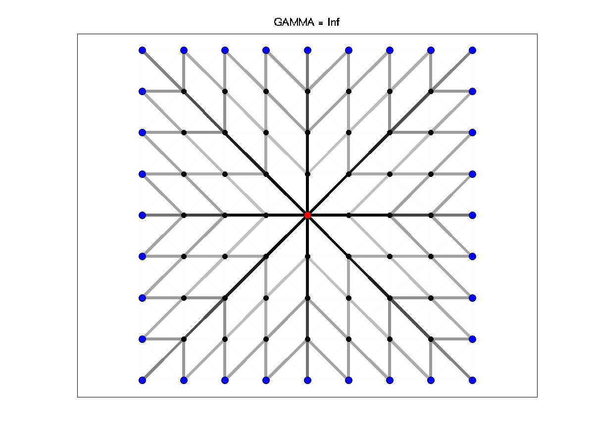
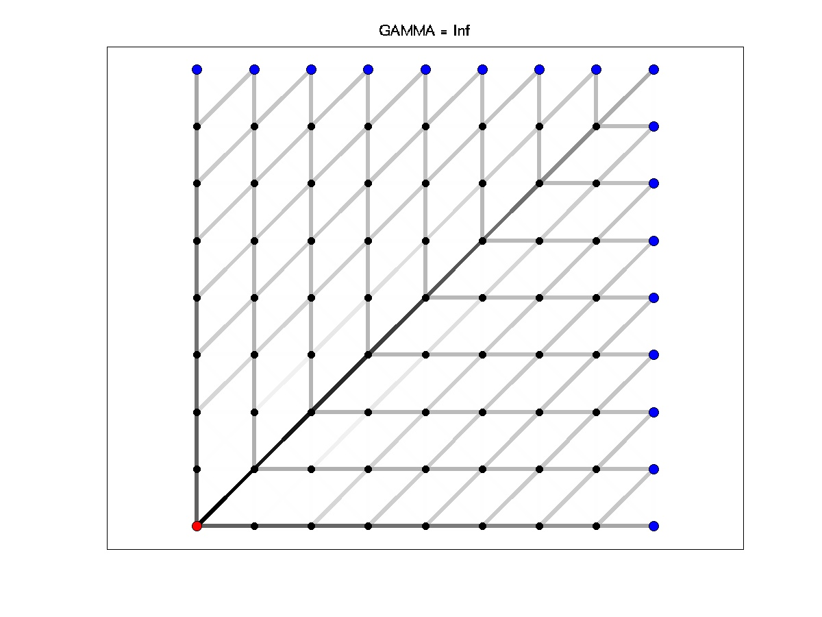
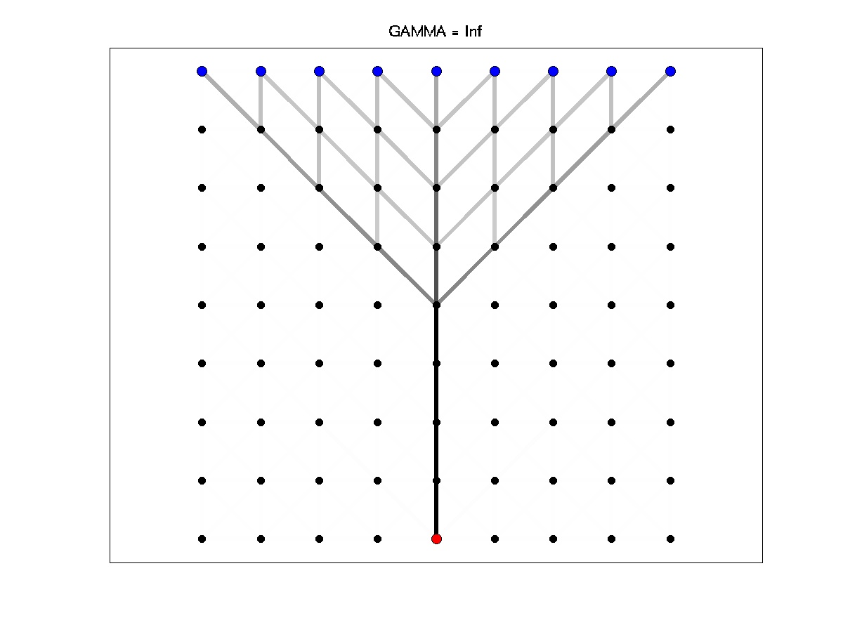
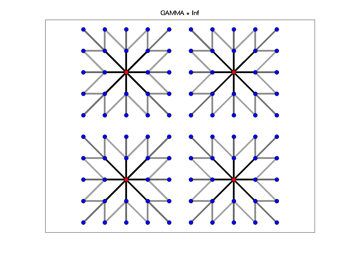
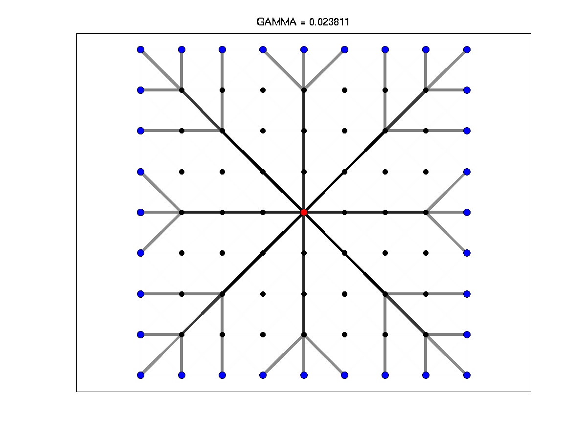
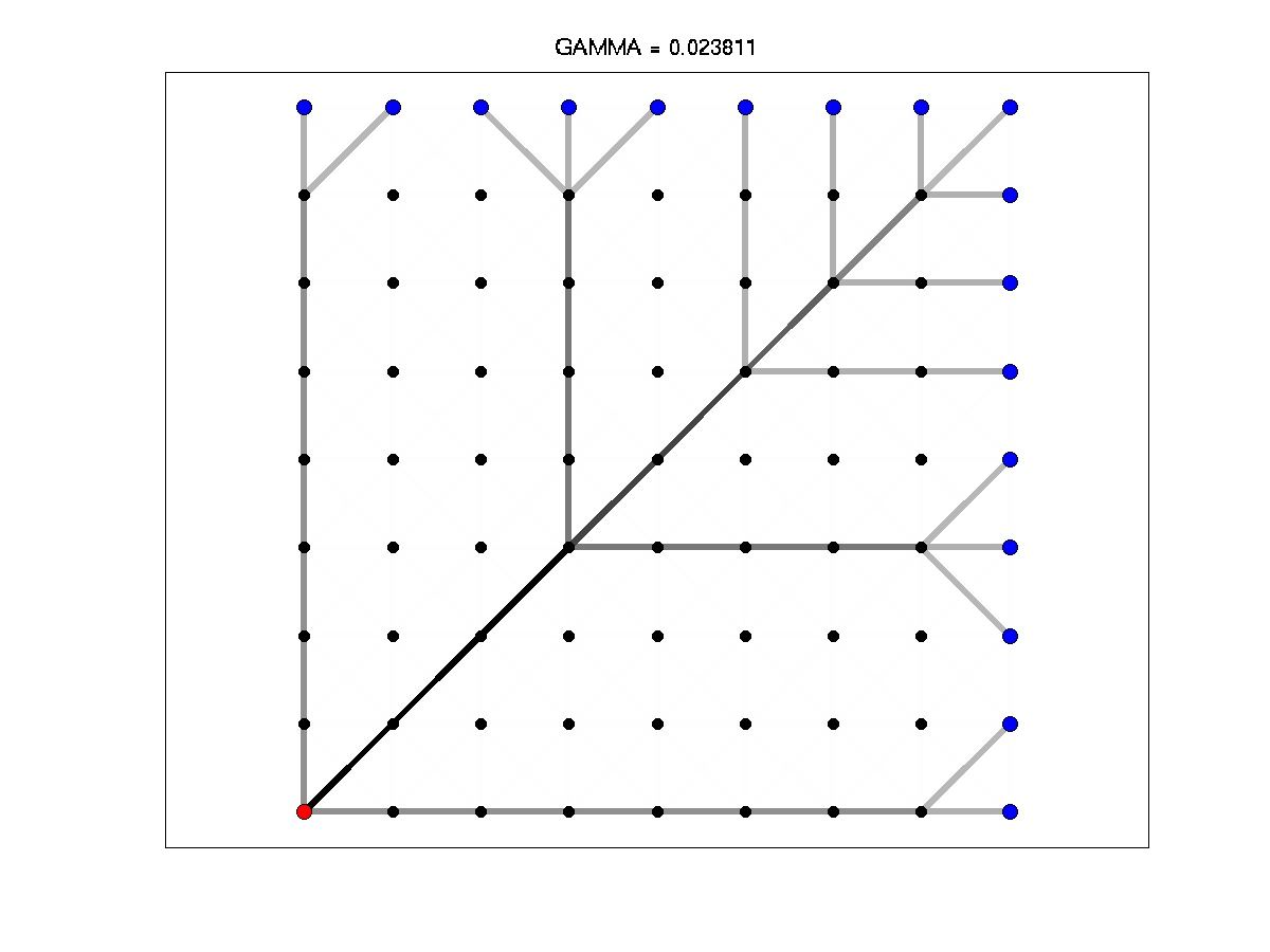
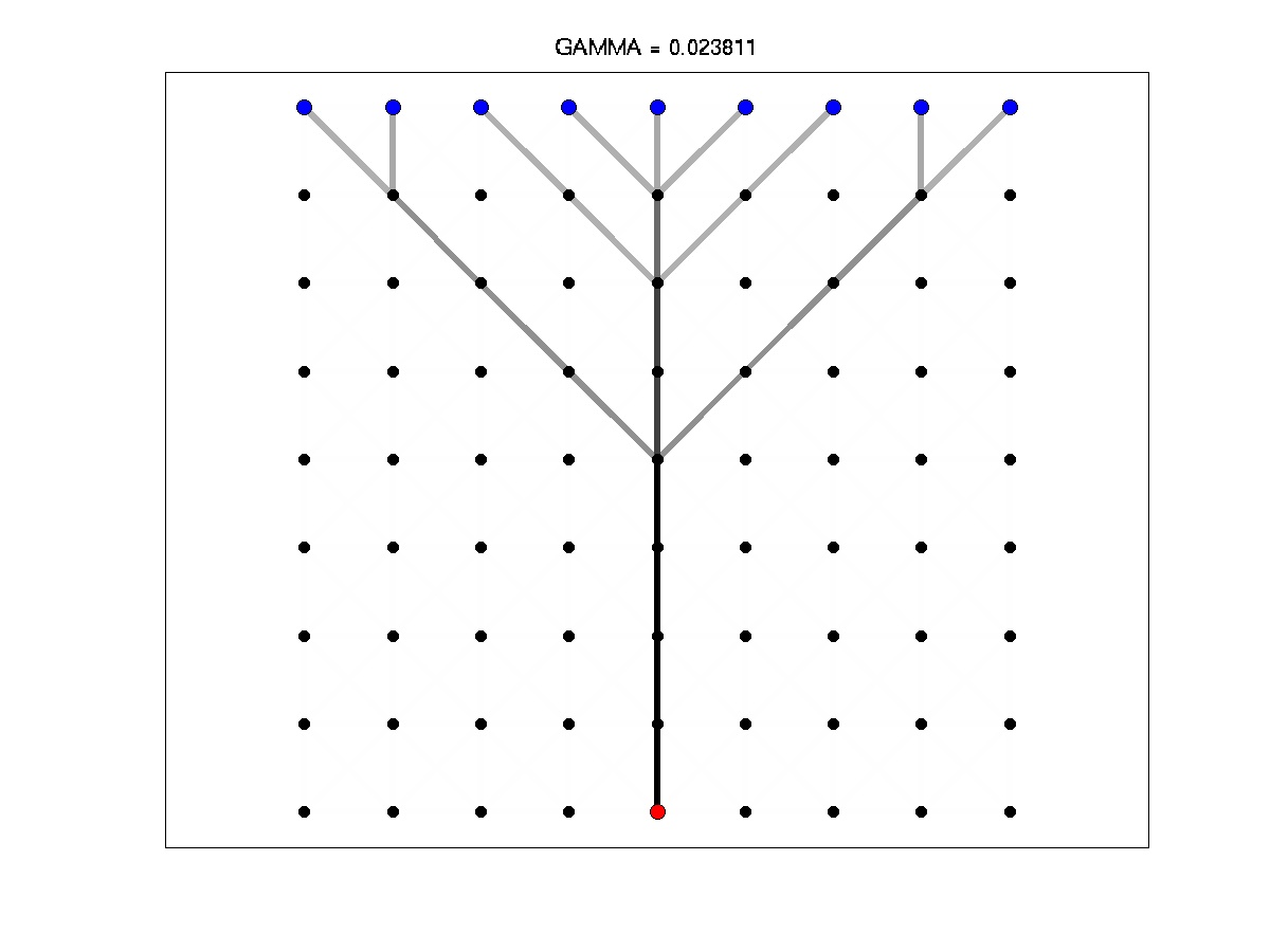
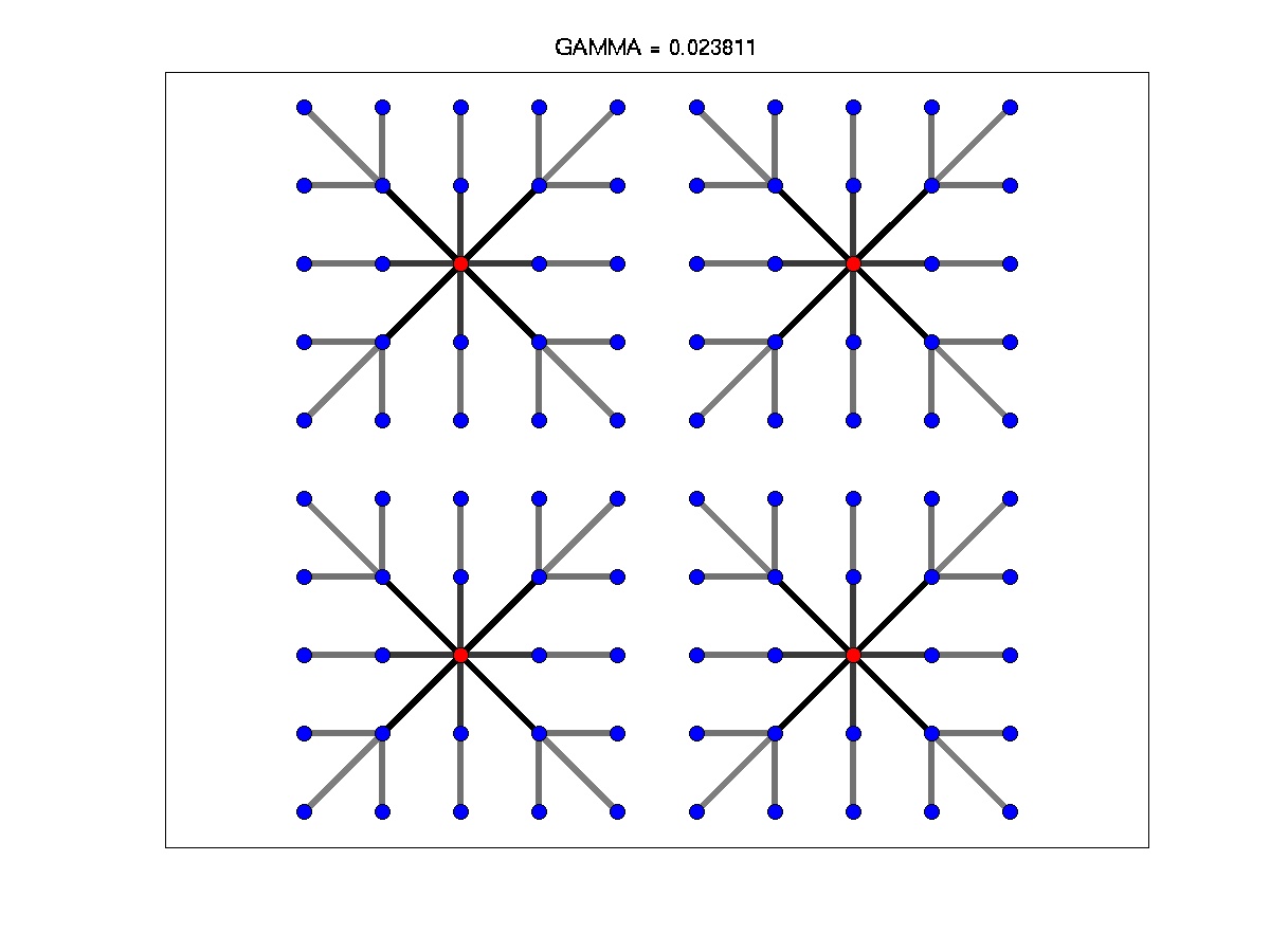
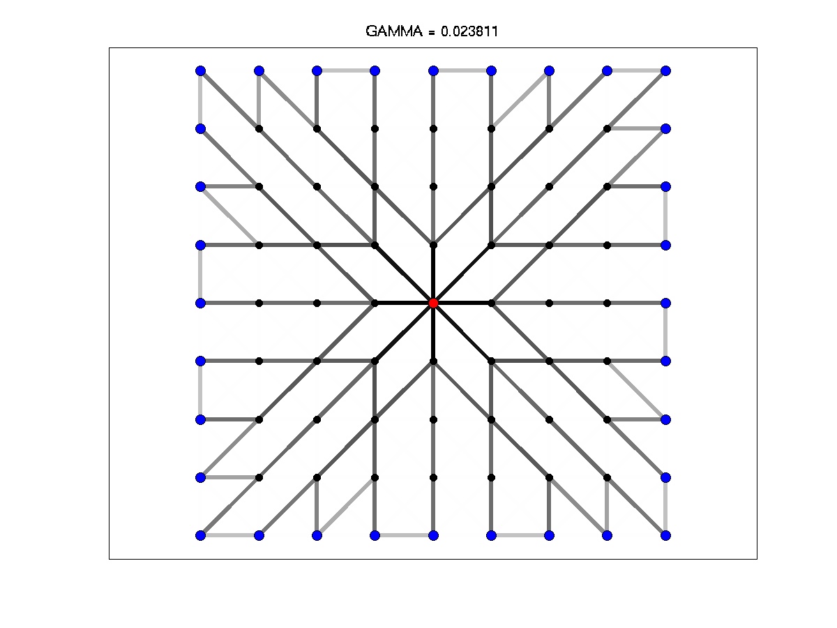
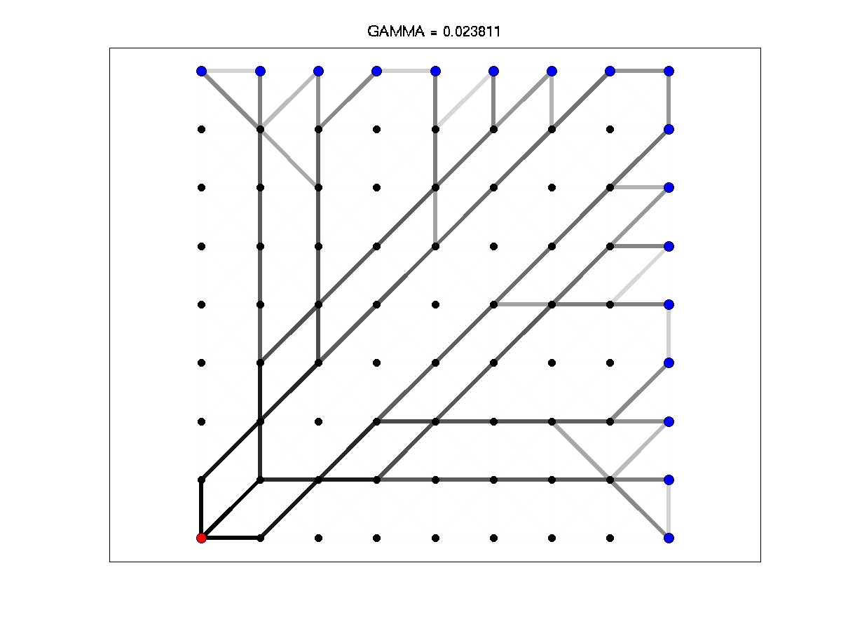
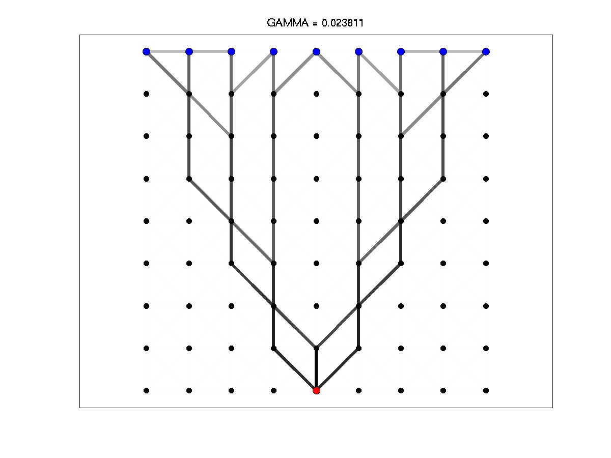
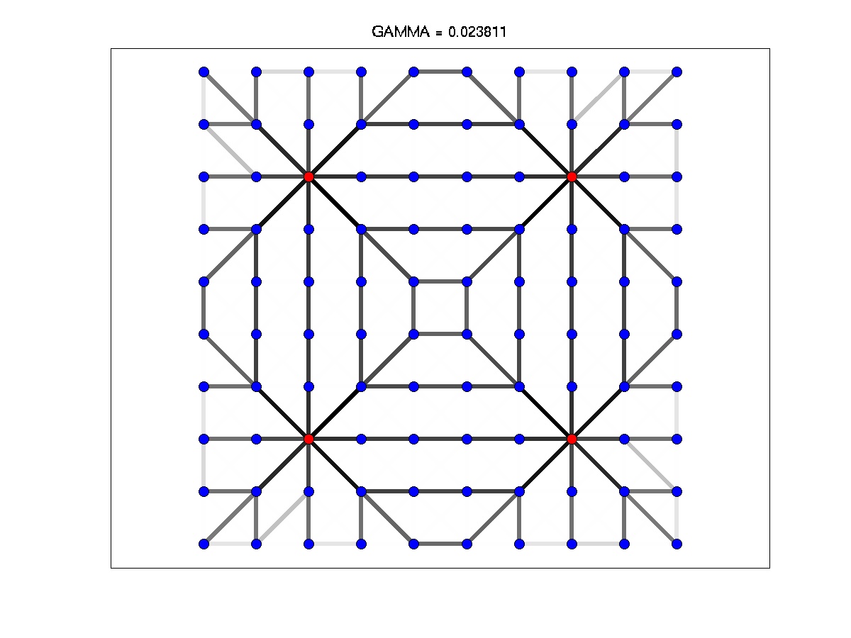
We now describe our fist set of demonstrations, based on four examples that we revisit in later sections. All examples having essentially the same graph topology but with different configurations of demand and generation nodes. The graph $G$ is comprised of a $w\times w$ grid of nodes (with $w=9$ or $10$) and has lines between nearest and second-nearest neighbors of the grid (resulting in vertical/horizontal edges between nearest neighbors and diagonal edges between second-nearest neighbors). Transmission, consumption and generation nodes are respectively marked as black dots, blue dots and red dots. We set $\alpha=1$ on horizontal/vertical edges and $\alpha=2$ on diagonal edges. We have $\bar{b}=-1$ and $\sigma=\tfrac{1}{3}$ at consumer nodes; and $\bar{b}=\sigma=0$ at transmission nodes. Fig. 1 shows the result of solving the convex network optimization in four examples. In the multiple generator case (seen at lower-right), we do not show the virtual generator or the lines to this generator. We observe that:

• The solution is somewhat sparse in these examples (it does not use all edges of $G$) but is not as sparse as possible (it is not a minimal tree/forest needed to connect consumers to generators).

• It is not necessary that all transmission nodes are involved in the solution, as shown by the example seen at the lower-left of the figure.

• With multiple generators (lower-right), the power transmission network may become disconnected, with each generator serving a particular subset of nearby consumer nodes.

Figure 1: Illustration of globally optimal network designs in the convex network optimization method. The strength of a line (conductance) is indicated by the darkness of the drawn edge, such that zero-conductance lines are not seen.

IV Selecting Network Structure

In this section we present a non-convex generalization of the approach taken in the preceding section. As we have seen, the convex optimization method does not always produce sparse solutions, i.e., it will typically use most of the edges of the graph $G$. In practical applications, we expect that such solutions are undesirable, as we would like to use the simplest network (with as few edges as possible) that is sufficient to meet power transmission requirements. Towards this end, we reformulate the network cost part of our optimization objective so as to favor solutions with fewer edges. However, this then gives a non-convex optimization problem, which is generally intractable to solve exactly. Hence, we develop a heuristic approach to find good solutions of this non-convex optimization problem. Using the majorization-minimization algorithm, we are able to approximately solve the non-convex problem by instead solving a sequence of convex optimization problems. Moreover, each convex optimization problem will be of the form solved in Section III, with the vector $\alpha$ being iteratively modified. Thus, the methods of Section III provide an optimization engine for the non-convex optimization method developed in this section.

IV-A Sparsity-Favoring Network Cost

In practice, we may also require that the network should by sparse. We formulate this by adding a cost on all lines with non-zero conductance so as to encourage solutions with as few lines as possible:

$$\min_{\theta\geq 0}\{\mathcal{L}(\theta)+\alpha^{T}\theta+\beta^{T}\phi(\theta)\}$$

where $\phi(t)$ is the unit-step function, $\phi(0)=0$ and $\phi(t)=1$ for all $t>0$, which is applied element-wise to $\theta$ such that $\beta^{T}\phi(\theta)=\sum_{\ell}\beta_{\ell}\phi(\theta_{\ell})$. Note the $\phi(t)$ is non-convex (in fact, it is concave on $t\geq 0$) and discontinuous at $t=0$,

Whereas the linear cost $\alpha^{T}\theta$ essentially represents the cost of copper needed to build the network, the non-convex cost $\beta^{T}\phi(\theta)$ represent other costs that do not scale with conductance, e.g., the cost of purchasing/leasing right-of-way along corridors of land along the lines and other expenses (labor, poles, towers, environmental impact) that do not tend to zero for low-conductance lines. More realistically, we expect the actual cost of a line to be a concave function of conductance approaching an affine function for large enough conductances. The simple model above roughly captures this behavior.

However, minimizing this discontinuous objective function is now a difficult combinatorial optimization problem. In order to find the optimal solution, one would need to enumerate all possible subgraphs of $G$ and perform a convex network optimization within each subgraph. Clearly this is not a scalable approach. We instead propose a heuristic solution method in the following subsections.

IV-B Annealed Smoothing Method

To avoid having to perform a combinatorial optimization, we begin by smoothing the objective function to a continuous (albeit non-convex) objective. This is accomplished by replacing the step function $\phi(t)$ by a continuous penalty function with smoothing parameter $\gamma>0$:

$$\phi_{\gamma}(t)=\frac{t}{t+\gamma}$$

We observe that $0\leq\phi_{\gamma}(t)\leq 1$ (for $t\geq 0$), $\phi_{\gamma}(0)=0$ and $\phi_{\gamma}(t)\rightarrow 1$ as $t\rightarrow\infty$. Hence, $\phi_{\gamma}$ may be regarded as a smooth approximation to the step function $\phi$. Moreover, $\phi_{\gamma}(t)\rightarrow\phi(t)$ as $\gamma\rightarrow 0$, such that the optimal solution of the smoothed problem should approach that of the combinatorial problem for sufficiently small $\gamma$. However, because this gives a non-convex optimization problem, there may be many local minima and it can still be intractable to determine the global minimum.

Next, we observe that for very large values of $\gamma$ we have $\phi_{\gamma}(t)\approx 0$ (over a large range of $t$) so that the smoothed problem becomes equivalent to the convex optimization problem. This suggests an “deterministic annealing” strategy in which we start with the solution of the tractable convex problem (corresponding to large $\gamma$) and then iteratively update the solution while gradually decreasing $\gamma$ to a small value (approximating the difficult combinatorial problem). At each stage of this annealing procedure, we must solve a non-convex minimization starting from an initial guess corresponding to a local minima of the preceding optimization.

IV-C Majorization-Minimization Algorithm

The approach described above requires solving (heuristically) a sequence of non-convex optimization problems. In this section, we present the algorithm used for this purpose. It is an instance of the general majorization-minimization algorithm [11], which we now review. Consider an objective function of the form

$$f(x)=f_{\cup}(x)+f_{\cap}(x)$$

where $f_{\cup}$ is a convex function and $f_{\cap}$ is a concave function. In order to seek a local minimum of $f$, one may iteratively linearize the concave part $f_{\cap}$ and minimize the resulting convex upper-bound to $f$. That is, given the previous guess $x^{(k)}$ of the solution, we may then approximate $f_{\cap}(x)$ by its linear upper-bound:

$$f_{\cap}(x)\leq f_{\cap}(x^{(k)})+\nabla f_{\cap}(x^{(k)})^{T}(x-x^{(k)}).$$

This gives a convex upper-bound approximation of the objective:

$$f(x)\leq f_{\cup}(x)+\nabla f_{\cap}(x^{(k)})^{T}x+\mathrm{const}$$

where $\mathrm{const}$ is independent of $x$. We then minimize this convex function to obtain the next guess:

$$x^{(k+1)}=\arg\min_{x}\left\{f_{\cup}(x)+\nabla f_{\cap}(x^{(k)})^{T}x\right\}.$$

This procedure is guaranteed not to increase the objective $f(x)$ and typically converges to a local minimum of $f(x)$. However, saddle-points and local maxima are also unstable fixed-points of the algorithm. Adding a small random perturbation to $x$ will cause the method to leave such non-minimal fixed-points.

It is straight-forward to apply this method in our present setting with $x=\theta$, $f_{\cup}(\theta)=\mathcal{L}(\theta)+\alpha^{T}\theta$ and $f_{\cap}(\theta)=\beta^{T}\phi_{\gamma}(\theta)$ (note that $\phi_{\gamma}(t)$ is concave). Doing so, we obtain the following iterative algorithm:

$$\alpha_{\ell}^{(k)} = \alpha_{\ell}+\tfrac{\gamma}{\left(\gamma+\theta^{(k-1)}_{\ell}\right)^{2}}\beta_{\ell}$$

$$\theta^{(k)} = \arg\min_{\theta\geq 0}\left\{\mathcal{L}(\theta)+(\alpha^{(k)})^{T}\theta\right\}$$ (7)

Observe that the optimization problem is of the same form that we considered in the Section III (with a modified value of $\alpha$) and can hence be solved using the methods of that section.

To accelerate convergence of the convex optimization algorithm, the parameter $\zeta$ of the barrier method may be kept fixed to a small value after the initial optimization. This is usually more efficient because small changes of the smoothing parameter $\gamma$ or the coefficient vector $\alpha$ typically do not produce a large change in the optimal $\theta$. However, occasionally it can happen that reducing $\gamma$ can cause a local minima to disappear, such that the algorithm must migrate to another local minima. When this happens, as indicated by Newton’s method not converging after a reasonable number of iterations, it is better to “restart” the barrier method with a large value of $\zeta$.

IV-D Demonstrations

We return to those four examples introduced in Section III-E. Setting $\beta=1$ on horizontal/vertical edges and $\beta=\sqrt{2}$ on diagonal edges, we obtain the solutions seen in Fig. 2 using the smoothed-annealing and majorization-minimization methods described in this section. In these examples, the graph is “thinned” to a minimal tree or forest sufficient to distribute power to consumer nodes from the generator(s). However, the level of thinning actually depends on the relative sizes of $\alpha$ and $\beta$, e.g., for smaller values of $\beta$ one can obtain intermediate solutions between those seen in Figs. 1 and 2.

Figure 2: Illustration of sparse network designs. Compare to Fig. 1.

V Robust Network Design

In this section we propose a simple modification of the methods of the previous sections to obtain network designs that are robust to the failure of lines and/or generator of the network.

V-A Imposing Robustness to Line/Generator Failures

First, we observe that the expected power loss $\mathcal{L}(\theta)$ acts as a kind of barrier function which enforces the constraint that the network must remaining connected such that every consumer node is connected to at least one generator node. For instance, if we gradually reduce $\theta$ to zero on any subset of edges that separates a consumer node from all generators, the power loss $\mathcal{L}(\theta)$ will tend to infinity.

Now, suppose that lines of the power network are subject to failures, meaning that the conductance of a line is set to zero. We would like for the network to still be able to supply the consumers and do so without large power dissipations (e.g., caused by having to route large currents through low-conductance lines after a failure). Let $z\in\{0,1\}^{m}$ be an indicator vector of line failures such that $z_{\ell}=1$ for failed lines and $z_{\ell}=0$ for operational lines. The power dissipation after removing failed lines is $\mathcal{L}(\theta;z)\triangleq\mathcal{L}((\mathbf{1}-z)\circ\theta)$. Suppose that we require that the network is robust to up to $k$ line failures. Then, the worst case power dissipation is:

$$\mathcal{L}^{\setminus k}(\theta)=\max_{\mathbf{1}^{T}z=k}\mathcal{L}(\theta;z)$$

Importantly, we note that this robust power dissipation is a convex function of $\theta$ because the point-wise maximum of a collection of convex functions is also a convex function. We may then design our power network so as to minimize the robust objective:

$$\min_{\theta\geq 0}\left\{\mathcal{L}^{\setminus k}(\theta)+\alpha^{T}\theta+\beta^{T}\phi(\theta)\right\}$$

Again using the annealed smoothing and majorization-minimization methods, this results in a sequence of convex optimization problem of the form $\min_{\theta}\left\{\mathcal{L}^{\setminus k}(\theta)+\tilde{\alpha}^{T}\theta\right\}$. We note that the robust power loss serves as a barrier function to ensure that the graph remains $(k+1)$-connected, such that every consumer node must be connected to the (virtual) generator by at least $k+1$ distinct paths.

Lastly, we remark that we may apply the same method in the multiple-generator setting by requiring robustness with respect to failures of lines to the virtual generator in the augmented network representation, which is equivalent to allowing for failures of generators.

V-B Gibbsian “Soft-Max” Optimization

While this approach results in a convex optimization problem, its solution using standard steepest descent methods such as Newton’s method is complicated by the fact that $\mathcal{L}^{\setminus k}$ is non-smooth (it is not everywhere differentiable). One could handle this using non-smooth optimization methods such as subgradient descent. However, these methods tend to converge slowly. We avoid this complication by using the Gibbsian “soft-max” function with smoothing parameter $\tau>0$:

$$\mathcal{L}^{\setminus k}_{\tau}(\theta)=\tau\log\sum_{\mathbf{1}^{T}z=k}\exp\left[\tau^{-1}\mathcal{L}(z;\theta)\right]$$

This is a smooth, convex function of $\theta$ and gives an upper-bound to $\mathcal{L}^{\setminus k}(\theta)$. Moreover, $\mathcal{L}^{\setminus k}_{\tau}\rightarrow\mathcal{L}^{\setminus k}$ (uniformly) as $\tau\rightarrow 0$. Thus, smooth convex optimization of $\mathcal{L}^{\setminus k}(\theta)$ provides a good approximation to the non-smooth convex optimization of $\mathcal{L}^{\setminus k}$ for sufficiently small values of $\tau$.

V-C Demonstrations

Again, we return to those four examples discussed previously in Sections III-E and IV-D. Using the smoothed robust power loss with $k=1$ and $\tau=.01$, we obtain the robust network solutions seen in Fig. 3 using the smoothed annealing and majorization-minimization methods. Observe that these graphs are two-connected, such that every consumer node is connected to the (virtual) generator nodes by at least two distinct paths. Also, the multiple generator solution is now a connected graph so as to be robust to failure of a generator.

Figure 3: Illustration of robust network designs. Compare to Fig. 2.

VI Summary and Future Work

In summary, we have developed an optimization approach to design electric power transmission networks with the aim of balancing network efficiency versus the cost of building the network. At the core of our methods lies a convex network optimization problem generalizing methods of [10, 5]. We also have proposed non-convex extensions of this basic line-sizing problem to further encourage network sparsity. This allows the heuristic design of the network structure $G$ by seeking a sparse solution within an over-complete graph. We developed a heuristic solution technique using smoothed annealing and majorization-minimization methods [1, 11, 6]. So far, the experimental results obtained by these methods in toy problems have yielded very reasonable networks that appear to be optimal or near-optimal solutions of the proposed optimization problem.

There are many possible extensions of the basic optimization model we have developed. We begin by listing some straight-forward extensions that may give a better fit to real-world applications:

• Modeling renewable power generation. This may be handled as we have treated consumer nodes, but with positive $\bar{b}_{i}$.

• Incorporating constraints on the maximum output of generators. This is especially relevant in the multiple-generator setting.

• Modeling power storage capabilities (e.g. hybrid and electric vehicles). These are nodes of the network that may absorb power from the network when there is a surplus and then re-emit this power when demand is high.

• Allowing for load shedding. For a number of reasons, it may become necessary that not all of the demand for power can be met so that load shedding becomes necessary. It would be good to treat this somehow both in our random current model and in how we model the handling of line and/or generator failures.

• Putting (convex) constraints on the power dissipation and/or current per line. These is important to avoid over-loading lines in the first place (to avoid cascading failures).

• Rather than designing networks from scratch, we may also plan extensions/upgrades to existing networks in a similar manner simply by including existing line conductances at no cost.

A less trivial direction to explore is that of directly treating the AC power flow problem (rather then using the leading order DC approximation). However, so far it is unclear if this can be usefully treated within a convex optimization framework.

Another direction to explore concerns developing more efficient algorithms. The methods we are using so far all involve convex optimization procedures with per-iteration complexity that grows essentially as $\mathcal{O}(n^{3})$ (fixing the degree of $G$). We anticipate that more scalable algorithms (e.g., $\mathcal{O}(n^{3/2})$ for planar or near-planar graphs) should be possible using formulations that introduce auxiliary variables so as to allow Newton’s method to use more efficient linear solvers (e.g. nested dissection) that exploit sparsity of the initial graph $G$.

References

- [1] A. Blake and A. Zisserman. Visual Reconstruction. MIT Press, Cambrdige, MA, 1987.
- [2] S. Bohn and M. Magnasco. Structure, scaling and phase transition in the optimal transport network. Physical Review Letters, 98, February 2007.
- [3] B. Bollobás. Modern Graph Theory. Graduate Texts in Mathematics. Springer, 1998.
- [4] S. Boyd and L. Vandenberghe. Convex Optimization. Cambridge University Press, Cambridge, UK, 2004.
- [5] S. Boyd, L. Vandenberghe, and A. El Gamal. Design of robust global power and ground networks. In ISPD ’01, 2001.
- [6] E. Candés, M. Wakin, and S. Boyd. Enhancing sparsity by reweighted minimization. The Journal of Fourier Analysis and Applications, 2008.
- [7] R. Chartrand. Exact reconstructions of sparse signals via nonconvex minimization. IEEE Signal Processing Letters, 14:707–710, 2007.
- [8] R. Chartrand and W. Yin. Iteratively reweighted algorithms for compressive sensing. In 33rd International Conference on Acoustics, Speech, and Signal Processing (ICASSP), 2008.
- [9] P. Doyle and J. Snell. Random Walks and Electric Networks. Mathematical Association of America, 1984.
- [10] A. Ghosh, S. Boyd, and A. Saberi. Minimizing effective resistance of a graph. SIAM Review, 50(1):37–66, 2008.
- [11] D. Hunter and K. Lange. A tutorial on MM algorithms. The American Statistician, 58(1):30–37, February 2004.
- [12] J. Idier. Convex half-quadratic criteria and interacting auxiliary variables for image reconstrution. IEEE transactions on image processing, 1001–1009(7), July 2001.
- [13] W. Short and N. Blair. wind energy by 2030: Increasing wind energy’s contribution to U.S. electricity supply. DOE Report No. DOE/GO-102008-2567, 2008.
- [14] W. Short, N. Blair, and D. Heimiller. Long-term potential of wind power in the United States. Solar Today, pages 28–29, 2003.
- [15] L. Toole, M. Fair, A. Berscheid, and R. Bent. Electric power transmission network design for wind generation in the western United States: Algorithms, methodology, and analysis. to appear in IEEE Conference on Distribution and Transmission, 2010.
- [16] A. Wood and B. Wollenberg. Power Generation Operation And Control. New York, second edition, 1996.