Results on numerics for FBSDE with drivers of quadratic growth

Abstract

We consider the problem of numerical approximation for forward-backward stochastic differential equations with drivers of quadratic growth (qgFBSDE). To illustrate the significance of qgFBSDE, we discuss a problem of cross hedging of an insurance related financial derivative using correlated assets. For the convergence of numerical approximation schemes for such systems of stochastic equations, path regularity of the solution processes is instrumental. We present a method based on the truncation of the driver, and explicitly exhibit error estimates as functions of the truncation height. We discuss a reduction method to FBSDE with globally Lipschitz continuous drivers, by using the Cole-Hopf exponential transformation. We finally illustrate our numerical approximation methods by giving simulations for prices and optimal hedges of simple insurance derivatives.

2000 AMS subject classifications: Primary: 60H10; Secondary: 60H07, 65C30.

Key words and phrases: backward stochastic differential equation; BSDE; forward-backward stochastic differential equation; FBSDE; driver of quadratic growth; utility maximization; exponential utility; utility indifference; pricing; hedging; entropic risk measure; insurance derivatives; securitization; differentiability; stochastic calculus of variations; Malliavin’s calculus; non-linear Feynman-Kac formula; Cole-Hopf transformation; BMO martingale; inverse Hölder inequality.

1 Introduction

Owing to their central significance in optimization problems for instance in stochastic finance and insurance, backward stochastic differential equations (BSDE), one of the most efficient tools of stochastic control theory, have been receiving much attention in the last 15 years. A particularly important class, BSDE with drivers of quadratic growth, for example, arise in the context of utility optimization problems on incomplete markets with exponential utility functions, or alternatively in questions related to risk minimization for the entropic risk measure. BSDE provide the genuinely stochastic approach of control problems which find their analytical expression in the Hamilton-Jacobi-Bellman formalism. BSDE with drivers of this type keep being a source of intensive research.

As Monte-Carlo methods to simulate random processes, numerical schemes for BSDE provide a robust method for simulating and approximating solutions of control problems. Much has been done in recent years to create schemes for BSDE with Lipschitz continuous drivers (see Bouchard and Touzi (2004) or Elie (2006) and references therein). The numerical approximation of BSDE with drivers of quadratic growth (qgBSDE) or systems of forward-backward stochastic equations with drivers of this kind (qgFBSDE) turned out to be more complicated. Only recently, in dos Reis (2009), one of the main obstacles was overcome. Following Bouchard and Touzi (2004) in the setting of Lipschitz drivers, the strategy to prove convergence of a numerical approximation combines two ingredients: regularity of the trajectories of the control component of a solution pair of the BSDE in the $L^{2}$-sense, a tool first investigated in the framework of globally Lipschitz BSDE by Zhang (2001), and a convenient a priori estimate for the solution. See Bouchard and Touzi (2004), Gobet et al. (2005), Delarue and Menozzi (2006) or Bender and Denk (2007) for numerical schemes of BSDE with globally Lipschitz continuous drivers, and an implementation of these ideas. The main difficulty treated in dos Reis (2009) consisted of establishing path regularity for the control component of the solution pair of the qgBSDE. For this purpose, the control component, known to be represented by the Malliavin trace of the other component, had to be thoroughly investigated in a subtle and complex study of Malliavin derivatives of solutions of BSDE. This study extends a thorough investigation of smoothness of systems of FBSDE by methods based on Malliavin’s calculus and BMO martingales independently conducted in Ankirchner et al. (2007b) and Briand and Confortola (2008). The knowledge of path regularity obtained this way is implemented in a second step of the approach in dos Reis (2009). The quadratic growth part of the driver is truncated to create a sequence of approximating BSDE with Lipschitz continuous drivers. Path regularity is exploited to explicitly capture the convergence rate for the solutions of the truncated BSDE as a function of the truncation height. The error estimate for the truncation, which is of high polynomial order, combines with the ones for the numerical approximation in any existent numerical scheme for BSDE with Lipschitz continuous drivers, to control the convergence of a numerical scheme for qgBSDE. It allows in particular to establish the convergence order for the approximation of the control component in the solution process.

An elegant way to avoid the difficulties related to drivers of quadratic growth, and to fall back into the setting of globally Lipschitz ones, consists of using a coordinate transform well known in related PDE theory under the name “exponential Cole-Hopf transformation”. The transformation eliminates the quadratic growth of the driver in the control component at the cost of producing a transformed driver of a new BSDE which in general lacks global Lipschitz continuity in the other component. This difficulty can be avoided by some structure hypotheses on the driver. Once this is done, the transformed BSDE enjoys global Lipschitz continuity properties. Therefore the problem of numerical approximation can be tackled in the framework of transformed coordinates by schemes well known in the Lipschitz setting. As stated before, this again requires path regularity results in the $L^{2}$-sense for the control component of the solution pair of the transformed BSDE. For globally Lipschitz continuous drivers Zhang (2001) provides path regularity under simple and weak additional assumptions such as $\frac{1}{2}$-Hölder continuity of the driver in the time variable. The smoothness of the Cole-Hopf transformation allows passing back to the original coordinates without losing path regularity. In summary, if one accepts the additional structural assumptions on the driver, the exponential transformation approach provides numerical approximation schemes for qgBSDE under weaker smoothness conditions for the driver.

In this paper we aim to give a survey of these two approaches to obtain numerical results for qgBSDE. Doing this, we always keep an eye on one of the most important applications of qgBSDE, which consists of providing a genuinely probabilistic approach to utility optimization problems for exponential utility, or equivalently risk minimization problems with respect to the entropic risk measure, that lead to explicit descriptions of prices and hedges. We motivate qgBSDE by reviewing a simple exponential utility optimization problem resulting from a method to determine the utility indifference price of an insurance related asset in a typical incomplete market situation, following Ankirchner et al. (2007b) and Frei (2009). The setting of the problem allows in particular the calculation of the driver of quadratic growth of the associated BSDE. After discussing the problem of numerical approximations, in this case by applying the method related to the exponential transform, we are finally able to illustrate our findings by giving some numerical simulations obtained with the resulting scheme.

The paper is organized as follows. In Section 2 we fix the notation used for treating problems about qgFBSDE and recall some basic results. Section 3 is devoted to presenting utility optimization problems used for pricing and hedging derivatives on non-tradable underlyings using correlated assets in a utility indifference approach. In section 4 we review smoothness results for the solutions processes of qgFBSDE, and apply them to show $L^{2}$-regularity of the control component of the solution process of a qgFBSDE. In Section 5 we discuss the truncation method for the quadratic terms of the driver to derive a numerical approximation scheme for qgFBSDE. Section 6 is reserved for a discussion of the applicability of the exponential transform in the qgBSDE setting. In Section 7 we return to the motivating pricing and hedging problem and use it as a platform for illustrating our results by numerical simulations.

2 Preliminaries

Fix $T\in\mathbb{R}_{+}=[0,\infty)$. We work on the canonical Wiener space $(\Omega,\mathcal{F},\mathbb{P})$ on which a $d$-dimensional Wiener process $W=(W^{1},\cdots,W^{d})$ restricted to the time interval $[0,T]$ is defined. We denote by $\mathcal{F}=(\mathcal{F}_{t})_{t\in[0,T]}$ its natural filtration enlarged in the usual way by the $\mathbb{P}$-zero sets.

Let $p\geq 2,m,d\in\mathbb{N}$, $\mathbb{Q}$ be a probability measure on $(\Omega,\mathcal{F})$. We use the symbol $\mathbb{E}^{\mathbb{Q}}$ for the expectation with respect to $\mathbb{Q}$, and omit the superscript for the canonical measure $\mathbb{P}$. To denote the stochastic integral process of an adapted process $Z$ with respect to the Wiener process on $[0,T]$, we write $Z*W=\int_{0}^{\cdot}Z_{s}\mathrm{d}W_{s}$.

For vectors $x=(x^{1},\cdots,x^{m})$ in Euclidean space $\mathbb{R}^{m}$ we denote $|x|=(\sum_{i=1}^{m}(x^{i})^{2})^{\frac{1}{2}}$. In our analysis the following normed vector spaces will play a role. We denote by

• $L^{p}(\mathbb{R}^{m};\mathbb{Q})$ the space of $\mathcal{F}_{T}$-measurable random variables $X:\Omega\mapsto\mathbb{R}^{m}$, normed by $\lVert X\lVert_{L^{p}}=\mathbb{E}^{\mathbb{Q}}[\,|X|^{p}]^{\frac{1}{p}}$; $L^{\infty}$ the space of bounded random variables;

• $\mathcal{S}^{p}(\mathbb{R}^{m})$ the space of all measurable processes $(Y_{t})_{t\in[0,T]}$ with values in $\mathbb{R}^{m}$ normed by $\|Y\|_{\mathcal{S}^{p}}=\mathbb{E}[\left(\sup_{t\in[0,T]}|Y_{t}|\right)^{p}]^{\frac{1}{p}}$; $\mathcal{S}^{\infty}(\mathbb{R}^{m})$ the space of bounded measurable processes;

• $\mathcal{H}^{p}(\mathbb{R}^{m},\mathbb{Q})$ the space of all progressively measurable processes $(Z_{t})_{t\in[0,T]}$ with values in $\mathbb{R}^{m}$ normed by $\|Z\|_{\mathcal{H}^{p}}=\mathbb{E}^{\mathbb{Q}}[\left(\int_{0}^{T}|Z_{s}|^{2}\mathrm{d}s\right)^{p/2}]^{\frac{1}{p}};$

• $BMO(\mathcal{F},\mathbb{Q})$ or $BMO_{2}(\mathcal{F},\mathbb{Q})$ the space of square integrable $\mathcal{F}$-martingales $\Phi$ with $\Phi_{0}=0$ and we set

  $$\lVert\Phi\lVert_{BMO(\mathcal{F},\mathbb{Q})}^{2}=\sup_{\tau}\Big{\|}\,\mathbb{E}^{\mathbb{Q}}\big{[}\langle\Phi\rangle_{T}-\langle\Phi\rangle_{\tau}|\mathcal{F}_{\tau}\big{]}\Big{\|}_{\infty}<\infty,$$

  where the supremum is taken over all stopping times $\tau\in[0,T]$. More details on this space can be found in Appendix 1. In case $\mathbb{Q}$ resp. $\mathcal{F}$ is clear from the context, we may omit the arguments $\mathbb{Q}$ or $\mathcal{F}$ and simply write $BMO(\mathbb{Q})$ resp. $BMO(\mathcal{F})$ etc;

• $\mathbb{D}^{k,p}(\mathbb{R}^{d})$ and $\mathbb{L}_{k,d}(\mathbb{R}^{d})$ the spaces of Malliavin differentiable random variables and processes, see Appendix 2.

In case there is no ambiguity about $m$ or $\mathbb{Q}$, we may omit the reference to $\mathbb{R}^{m}$ or $\mathbb{Q}$ and simply write $\mathcal{S}^{\infty}$ or $\mathcal{H}^{p}$ etc.

We investigate systems of forward diffusions coupled with backward stochastic differential equations with quadratic growth in the control variable (qgFBSDE for short), i.e. given $x\in\mathbb{R}^{m}$, $t\in[0,T]$, and four continuous measurable functions $b$, $\sigma$, $g$ and $f$ we analyze systems of the form

$$X^{x}_{t} =x+\int_{0}^{t}b(s,X^{x}_{s})\mathrm{d}s+\int_{0}^{t}\sigma(s,X^{x}_{s})\mathrm{d}W_{s},$$ (1)

$$Y^{x}_{t} =g(X^{x}_{T})+\int_{t}^{T}f(s,X^{x}_{s},Y^{x}_{s},Z^{x}_{s})\mathrm{d}s-\int_{t}^{T}Z^{x}_{s}\mathrm{d}W_{s}.$$ (2)

In case there is no ambiguity about the initial state $x$ of the forward system, we may and do suppress the superscript $x$ and just write $X,Y,Z$ for the solution components. For the coefficients of this system we make the following assumptions:

•     There exists a positive constant $K$ such that $b,\sigma_{i}:[0,T]\times\mathbb{R}^{m}\to\mathbb{R}^{m},1\leq i\leq d,$ are uniformly Lipschitz continuous with Lipschitz constant $K$, and $b(\cdot,0)$ and $\sigma_{i}(\cdot,0),1\leq i\leq d,$ are bounded by $K$.

  There exists a constant $M\in\mathbb{R}_{+}$ such that $g:\mathbb{R}^{m}\to\mathbb{R}$ is absolutely bounded by $M$, $f:[0,T]\times\mathbb{R}^{m}\times\mathbb{R}\times\mathbb{R}^{d}\to\mathbb{R}$ is measurable and continuous in $(x,y,z)$ and for $(t,x)\in[0,T]\times\mathbb{R}^{m}$, $y,y^{\prime}\in\mathbb{R}$ and $z,z^{\prime}\in\mathbb{R}^{d}$ we have

  $$|f(t,x,y,z)| \leq M(1+|y|+|z|^{2}),$$

  $$|f(t,x,y,z)-f(t,x,y^{\prime},z^{\prime})| \leq M\Big{\{}|y-y^{\prime}|+(1+|z|+|z^{\prime}|)|z-z^{\prime}|\Big{\}}.$$

The theory of SDE is well established. Since we wish to focus on the backward equation component of our system we emphasize that the relevant results for SDE are summarized in Appendix 3.

Theorem 2.1 (Properties of qgFBSDE).

Under (H0), the system (1), (2) has a unique solution $(X,Y,Z)\in\mathcal{S}^{2}\times\mathcal{S}^{\infty}\times\mathcal{H}^{2}$. The respective norms of $Y$ and $Z$ can be dominated from above by constants depending only on $T$ and $M$ as given by assumption (H0). Furthermore

$$Z*W=\int_{0}^{.}Z_{s}\mathrm{d}W_{s}\in BMO(\mathbb{P})\textrm{ and hence for all }p\geq 2\textrm{ one has }Z\in\mathcal{H}^{p}.$$

It is possible to go beyond the bounded terminal condition hypothesis by imposing the existence of all its exponential moments instead. In this case $Z*W$ is no longer in $BMO$. As we shall see in Section 4, the $BMO$ property of $Z*W$ plays a crucial role in all of our smoothness results for systems of FBSDE. It combines with the inverse Hölder inequality for the exponentials generated by $BMO$ martingales to control moments of functionals of the solutions of FBSDE. Smoothness of solutions is instrumental for instance in estimates for numerical approximations of solutions.

3 Pricing and hedging with correlated assets

The pivotal task of mathematical finance is to provide solid foundations for the valuation of contingent claims. In recent years, markets have displayed an increasing need for financial instruments pegged to non-tradable underlyings such as temperature and energy indices or toxic matter emission rates. In the same manner as liquidly traded underlyings, securities on non-tradable underlyings are used to measure, control and manage risks, as well as to speculate and take advantage of market imperfections. Since non-tradability produces residual risks which are innate and inaccessible to hedging, institutional investors look for tradable assets which are correlated to the non-tradable ones. In incomplete markets, one established pricing paradigm is the utility maximization principle. Upon choosing a risk preference, investors evaluate contingent claims by replicating according to an investment strategy that yields the most favorable utility value. Interplays and connections between the pricing of contingent claims on non-tradable underlyings and the theory of qgFBSDE were studied, among others, by Ankirchner et al. (2007a), Morlais (2009), Imkeller et al. (2009), and recently by Frei (2009). Based on this setup, we consider the problem of numerically evaluating contingent claims based on non-tradable underlyings. This will be done by intervention of the exponential transformation of qgBSDE, to be introduced in Section 6. It allows to work under weaker assumptions than the numerical schemes for qgFBSDE based on the results reviewed in Section 4, and will allow some illustrative numerical simulations in Section 7.

The following toy market setup can be found in Section 4 of Frei (2009). Assume $d=2$, so that $W=(W^{1},W^{2})$ is our basic two-dimensional Brownian motion. We use them to define a third Brownian motion $W^{3}$ correlated to $W^{1}$ with respect to a correlation coefficient $\rho\in[-1,1]$ according to

$$W^{3}_{s} :=\int_{0}^{s}\rho\mathrm{d}W^{1}_{u}+\int_{0}^{s}\sqrt{1-\rho^{2}}\mathrm{d}W^{2}_{u},\leavevmode\nobreak\ \leavevmode\nobreak\ 0\leq s\leq T.$$

Contingent claims are assumed to be tied to a one-dimensional non-tradable index that is subject to

$$\mathrm{d}R_{t} =\mu(t,R_{t})\mathrm{d}t+\sigma(t,R_{t})\mathrm{d}W^{1}_{t},\leavevmode\nobreak\ R_{0}=r_{0}>0,$$ (3)

where $\mu,\sigma:[0,T]\times\mathbb{R}\to\mathbb{R}$ are deterministic measurable and uniformly Lipschitz continuous functions, uniformly of (at most) linear growth in their state variable. The securities market is governed by a risk free bank account yielding zero interest and one correlated risky asset whose dynamics (with respect to the zero interest bank account numéraire) are governed by

$$\frac{\mathrm{d}S_{s}}{S_{s}} =\alpha(s,R_{s})\mathrm{d}s+\beta(s,R_{s})\mathrm{d}W^{3}_{s},\leavevmode\nobreak\ S_{0}=s_{0}>0.$$ (4)

In compliance with Ankirchner et al. (2007a), we assume that $\alpha,\beta:[0,T]\times\mathbb{R}\to\mathbb{R}$ are bounded and measurable functions, and furthermore $\beta^{2}(t,r)\geq\varepsilon>0$ holds uniformly for some fixed $\varepsilon>0$. Next, we set

$$\theta(s,r) :=\frac{\alpha(s,r)}{\beta(s,r)},\leavevmode\nobreak\ \leavevmode\nobreak\ (s,r)\in[0,T]\times\mathbb{R},$$

and note that the conditions on $\alpha$ and $\beta$ imply that $\theta$ is uniformly bounded.

An admissible investment strategy is defined to be a real-valued, measurable predictable process $\lambda$ such that $\int_{0}^{T}\lambda^{2}_{u}\mathrm{d}u<\infty$ holds $\mathbb{P}$-almost surely and such that the family

$$\left\{e^{-\eta\int_{0}^{\tau}\lambda_{u}\frac{dS_{u}}{S_{u}}}:\tau\leavevmode\nobreak\ \text{stopping time with values in}\leavevmode\nobreak\ [0,T]\right\}$$ (5)

is uniformly integrable. The set of all admissible investment strategies is denoted by $\mathcal{A}$. In the following, let $t\in[0,T]$ denote a fixed time. Then the set of all admissible investment strategies living on the time interval $[t,T]$ is defined analogously and we denote it by $\mathcal{A}_{t}$. Let $v_{t}$ denote the investor’s initial endowment at time $t$, that is, $v_{t}$ is an $\mathcal{F}_{t}$-measurable bounded random variable. The gain of the investor at time $s\in[t,T]$, denoted by $G_{s}$, is subject to trading according to investing $\lambda$ into the risky asset, and therefore given by

$$\mathrm{d}G^{\lambda}_{s} =\lambda_{s}\frac{dS_{s}}{S_{s}},\leavevmode\nobreak\ G_{t}=0.$$

We focus on European style contingent claims, i.e. payoff profiles resuming the form $F(R_{T})$ where we assume, in accordance with Ankirchner et al. (2007a), that $F:\mathbb{R}\to\mathbb{R}$ is measurable and bounded. Moreover the investor’s risk assessment presumes that her utility preference is reflected by the exponential utility function, so given a nonzero constant risk attitude parameter $\eta$, the investor’s utility function is

$$U(x) =-e^{-\eta x},\leavevmode\nobreak\ x\in\mathbb{R}.$$

The evolution of the investor’s portfolio over the time interval $[t,T]$ consists of her initial endowment $v_{t}$, her gains (or losses) via her investment into the risky asset under an investment strategy $\lambda$ and holding one share of the contingent claim $F(R_{T})$. Her objective is to find an investment strategy such that her time-$t$ utility is maximized, i.e. her maximization problem is given by

$$V^{F}_{t}(v_{t}) :=\sup\left\{\mathbb{E}\left[U(v_{t}+G^{\lambda}_{T}+F(R_{T}))\big{|}\mathcal{F}_{t}\right]:\lambda\in\mathcal{A}_{t}\right\}$$

$$=\exp\left\{-\eta v_{t}\right\}\sup\left\{\mathbb{E}\left[U(G^{\lambda}_{T}+F(R_{T}))\big{|}\mathcal{F}_{t}\right]:\lambda\in\mathcal{A}_{t}\right\}$$ (6)

For the sake of notational convenience, we write

$$V_{t}^{F}:=V_{t}^{F}(0)=\sup\left\{\mathbb{E}\left[U(G^{\lambda}_{T}+F(R_{T}))\big{|}\mathcal{F}_{t}\right]:\lambda\in\mathcal{A}_{t}\right\}.$$ (7)

Now pricing $F(R_{T})$ within the utility maximization paradigm is based on the identity

$$V^{0}_{t}(v_{t})=V^{F}_{t}(v_{t}-p_{t}),$$

where $V^{0}_{t}(v_{t})$ denotes the time-$t$ utility with initial endowment $v_{t}$ and with $F=0$ (see also Section 2 of Ankirchner et al. (2007a) and Section 3 of Frei (2009)). According to this identity, the investor is indifferent about a portfolio with initial endowment $v_{t}$ without receiving one quantity of the contingent claim $F(R_{T})$ and a portfolio with initial endowment $v_{t}-p_{t}$, now receiving one quantity of the contingent claim in addition. Hence $p_{t}$ is interpreted as the time-$t$ indifference price of the contingent claim $F(R_{T})$. By the equality $V^{F}_{t}(v_{t})=\exp\left\{-\eta v_{t}\right\}V_{t}^{F}$, it follows that

$$p_{t}=\frac{1}{\eta}\log\frac{V^{0}_{t}}{V_{t}^{F}},$$ (8)

which means that the indifference price does not depend on the initial endowment $v_{t}$. Since the time-$t$ indifference price (8) is fully characterized by $V^{0}_{t}$ and $V^{F}_{t}$, the focus now lies in the investigation of (3). In fact, Ankirchner et al. (2007a) and Frei (2009) have already pointed out that (7) yields a characterization by means of a qgFBSDE. In accordance with Frei (2009), let us denote by $(\mathcal{G}_{u})_{0\leq u\leq T}$ the filtration generated by $W^{1}$, completed by $\mathbb{P}$-null sets. Frei (2009)’s main ideas for rephrasing (3) in terms of a qgBSDE are summarized in the following

Lemma 3.1.

The qgFBSDE

$$Y_{s} = \leavevmode\nobreak\ \leavevmode\nobreak\ F(R_{T})+\int_{s}^{T}f(u,R_{u},Z_{u})\mathrm{d}u-\int_{s}^{T}Z_{u}\mathrm{d}W^{1}_{u},\quad s\in[0,T],$$ (9)

$$f(u,r,z)\leavevmode\nobreak\ = \leavevmode\nobreak\ \leavevmode\nobreak\ \frac{\theta^{2}(u,r)}{2\eta}-z\rho\theta(u,r)-\frac{\eta}{2}\left(1-\rho^{2}\right)z^{2},$$ (10)

has a unique solution $(Y,Z)\in\mathcal{S}^{\infty}\times\mathcal{H}^{2}$ such that $V^{F}_{t}=-e^{-\eta Y_{t}}$ holds $\mathbb{P}$-almost surely.

Proof.

Since $\theta(\cdot,r)$ is uniformly bounded and $\mathcal{G}$-predictable, the driver of (9) satisfies the conditions of Kobylanski (2000); thus (9) admits a unique solution $(Y,Z)\in\mathcal{S}^{\infty}\times\mathcal{H}^{2}$. Moreover, Mania and Schweizer (2005) have shown that $Z*W^{1}$ is both a BMO($\mathcal{F}$)- and BMO($\mathcal{G}$)-martingale. See also Ankirchner et al. (2007a). To prove the identity $V^{F}_{t}=-e^{-\eta Y_{t}}$, we notice that

$$e^{-\eta\left(G^{\lambda}_{T}+Y_{T}\right)} =e^{-\eta G^{\lambda}_{t}}e^{-\eta Y_{t}}e^{-\eta\left(Y_{T}-Y_{t}\right)}e^{-\eta\left(G^{\lambda}_{T}-G^{\lambda}_{t}\right)}$$

$$=e^{-\eta Y_{t}}e^{-\eta\left(Y_{T}-Y_{t}\right)}e^{-\eta\left(G^{\lambda}_{T}-G^{\lambda}_{t}\right)},$$

because $G^{\lambda}_{t}=0$. We then have

$$\exp\left\{-\eta\left(Y_{T}-Y_{t}\right)\right\}\exp\{-\eta(G^{\lambda}_{T}-G^{\lambda}_{t})\}$$

$$\qquad=\exp\left\{-\eta\left(\int_{t}^{T}Z_{u}\mathrm{d}W^{1}_{u}+\int_{t}^{T}\lambda_{u}\beta(u,R_{u})\mathrm{d}W^{3}_{u}+\int_{t}^{T}\left[\lambda_{u}\alpha(u,R_{u})-f(u,R_{u},Z_{u})\right]\mathrm{d}u\right)\right\}.$$

Denoting $\mathcal{E}_{t}^{s}(M)=\mathcal{E}(M)_{s}/\mathcal{E}(M)_{t}$ for $t\leq s\leq T$ where $\mathcal{E}(M)_{s}$ is the stochastic exponential of a given semi-martingale $M$, we introduce

$$K_{u}:=\frac{1}{2}\Big{(}\eta\left(\rho Z_{u}+\beta(u,R_{u})\lambda_{u}\right)-\theta_{u}\Big{)}^{2},\leavevmode\nobreak\ \leavevmode\nobreak\ t\leq u\leq T.$$

Then a simple calculation yields

$$\exp\Big{\{}-\eta\big{(}Y_{T}-Y_{t}\big{)}\Big{\}}\exp\Big{\{}-\eta\big{(}G^{\lambda}_{T}-G^{\lambda}_{t}\big{)}\Big{\}}$$

$$\qquad\qquad=\mathcal{E}_{t}^{T}\left(\int-\eta Z\mathrm{d}W^{1}-\int\eta\lambda\beta(\cdot,R)\mathrm{d}W^{3}\right)\exp\left\{\int_{t}^{T}K_{u}\mathrm{d}u\right\}.$$

Since $\lambda\beta(\cdot,R)*W^{3}$ is a BMO-martingale, we can condition with respect to the $\sigma$-algebra $\mathcal{F}_{t}$ and get

$$\mathbb{E}\left[e^{-\eta\left(G^{\lambda}_{T}+F(R_{T})\right)}\leavevmode\nobreak\ \big{|}\leavevmode\nobreak\ \mathcal{F}_{t}\right] =e^{-\eta Y_{t}}e^{\int_{t}^{T}K_{u}\mathrm{d}u}\geq e^{-\eta Y_{t}}.$$ (11)

By (5) and a localization argument, this inequality holds for every $\lambda\in\mathcal{A}_{t}$, and therefore we have $V^{F}_{t}\leq-e^{-\eta Y_{t}}$. To prove equality, note that the inequality (11) becomes an equality for $\tilde{\lambda}_{u}=-\frac{\rho}{\beta(u,R_{u})}Z_{u}+\frac{\theta(u,R_{u})}{\eta\beta(u,R_{u})}$; this in conjunction with the observation that

$$\exp\left\{-\eta\tilde{\lambda}_{u}\frac{dS_{u}}{S_{u}}\right\} =\exp\left\{-\eta G^{\tilde{\lambda}}_{T}\right\}=\exp\left\{-\eta\left(G^{\tilde{\lambda}}_{T}-G^{\tilde{\lambda}}_{t}\right)\right\}$$

$$=\mathcal{E}_{t}^{T}\left(\int-\eta Z\mathrm{d}W^{1}-\int\eta\tilde{\lambda}\beta(\cdot,R)\mathrm{d}W^{3}\right)\times\exp\left\{-\eta\left(Y_{T}-Y_{t}\right)\right\}$$

is the product of a bounded process and true $\mathcal{F}$-martingale yields that condition (5) is satisfied. Hence $\tilde{\lambda}\in\mathcal{A}_{t}$ and we have shown $V^{F}_{t}=-e^{-\eta Y_{t}}$. ∎

The proof of the previous Lemma 3.1 yields the following

Corollary 3.2.

The investment strategy

$$\tilde{\lambda}_{s}:=-\frac{\rho}{\beta(s,R_{s})}Z_{s}+\frac{\theta(s,R_{s})}{\eta\beta(s,R_{s})},\leavevmode\nobreak\ \leavevmode\nobreak\ t\leq s\leq T,$$ (12)

where $Z$ is the control component of the solution to (9), belongs to $\mathcal{A}_{t}$ and satisfies

$$\mathbb{E}\left[U(v_{t}+G^{\tilde{\lambda}_{T}}+F(R_{T})\big{|}\mathcal{F}_{t}\right] =\sup\left\{\mathbb{E}\left[U(v_{t}+G^{\lambda}_{T}+F(R_{T})\big{|}\mathcal{F}_{t}\right]:\lambda\in\mathcal{A}_{t}\right\}=V^{F}_{t}(v_{t}).$$

One application is given in the following example.

Example 3.3.

[Put option on kerosene, compare with Example 1.2 from Ankirchner et al. (2007a)] Facing recent considerable declines in world oil prices, companies producing kerosene wish to partially cover their risk of such a depreciation. European put options are an established financial instrument to comply with this demand of risk covering. Since kerosene is not traded in a liquid market, derivative contracts on this underlying must be arranged on an over-the-counter basis. Knowing that the price of heating oil is highly correlated with the price of kerosene, the pricing and hedging of a European put option on kerosene can be done by a dynamic investment in (the liquid market of) heating oil. A numerical treatment of this pricing problem will be displayed in Section 7.

4 Smoothness and path regularity results

The principal aim of this paper is to survey some recent results on the numerical approximation of prices and hedging strategies of financial derivatives such as the liability $F(R_{T})$ in the setting of the previous section. As we saw, this leads us directly to qgFBSDE. In the subsequent sections we shall discuss an approach based on a truncation of the driver’s quadratic part in the control variable. It will be crucial to give an estimate for the error committed by truncating. Our error estimate will be based on smoothness results for the control component $Z^{x}$ of solutions of the BSDE part of our system. Smoothness is understood both in the sense of regular sensitivity to initial states $x$ of the forward component, as well as in the sense of the stochastic calculus of variations. Since the control component of the solution of a BSDE is related to the Malliavin trace of the other component, we will be led to look at variational derivatives of the first order.

Our first result concerns the smoothness of the map $[0,T]\times\mathbb{R}^{m}\ni(t,x)\mapsto Z_{t}^{x}$, especially its differentiability in $x$. The second result refers to the variational differentiability of $(Y^{x},Z^{x})$ in the sense of Malliavin’s calculus. We shall work under the following hypothesis, where we denote the gradient by the common symbol $\nabla$, and by $\nabla_{u}$ if we wish to emphasize the variable $u$ with respect to which the derivative is taken.

•     Assume that (H0) holds. For any $0\leq t\leq T$ the functions $b(t,\cdot),\sigma_{i}(t,\cdot),1\leq i\leq d,$ are continuously differentiable with bounded derivatives in the spatial variable. There exists a positive constant $c$ such that

  $$y^{T}\sigma(t,x)\sigma^{T}(t,x)y\geq c|y|^{2},\quad x,y\in\mathbb{R}^{m},\ t\in[0,T].$$ (13)

  $f$ is continuously partially differentiable in $(x,y,z)$ and there exists $M\in\mathbb{R}_{+}$ such that for $(t,x,y,z)\in[0,T]\times\mathbb{R}^{m}\times\mathbb{R}\times\mathbb{R}^{d}$

  $$|\nabla_{x}f(t,x,y,z)| \leq M(1+|y|+|z|^{2}),$$

  $$|\nabla_{y}f(t,x,y,z)| \leq M,$$

  $$|\nabla_{z}f(t,x,y,z)| \leq M(1+|z|).$$

  $g:\mathbb{R}^{m}\to\mathbb{R}$ is a continuously differentiable function satisfying $|\nabla g|\leq M$.

Smoothness results

The following differentiability results are extensions of Theorems proved in Ankirchner et al. (2007b) and Briand and Confortola (2008). For further details, comments and complete proofs we refer to the mentioned works or to dos Reis (2009).

Theorem 4.1 (Classical differentiability).

Suppose that (H1) holds. Then for all $p\geq 2$ the solution process $\Theta^{x}=(X^{x},Y^{x},Z^{x})$ of the qgFBSDE (1), (2) with initial vector $x\in\mathbb{R}^{m}$ for the forward component belongs to $\mathcal{S}^{p}\times\mathcal{S}^{p}\times\mathcal{H}^{p}$. The application $\mathbb{R}^{m}\ni x\mapsto(X^{x},Y^{x},Z^{x})\in\mathcal{S}^{p}(\mathbb{R}^{m})\times\mathcal{S}^{p}(\mathbb{R})\times\mathcal{H}^{p}(\mathbb{R}^{d})$ is differentiable. The derivatives of $x\mapsto X^{x}$ satisfy (21) while the derivatives of the map $x\mapsto(Y^{x},Z^{x})$ satisfy the linear BSDE

$$\nabla Y_{t}^{x} =\nabla g(X_{T}^{x})\nabla X^{x}_{T}-\int_{t}^{T}\nabla Z_{s}^{x}\mathrm{d}W_{s}+\int_{t}^{T}\langle\nabla f(s,\Theta^{x}_{s}),\nabla\Theta^{x}_{s}\rangle\mathrm{d}s,\quad t\in[0,T].$$

Theorem 4.2 (Malliavin differentiability).

Suppose that (H1) holds. Then the solution process $(X,Y,Z)$ of FBSDE (1), (2) has the following properties. For $x\in\mathbb{R}^{m}$,

• $X^{x}$ satisfies (22) and for any $0\leq t\leq T$, $x\in\mathbb{R}^{m}$ we have $(Y^{x},Z^{x})\in\mathbb{L}_{1,2}\times\big{(}\mathbb{L}_{1,2}\big{)}^{d}$. $X^{x}$ fulfills the statement of Theorem 7.4, and a version of $(D_{u}Y^{x}_{t},D_{u}Z^{x}_{t})_{0\leq u,t\leq T}$ satisfies

  $$D_{u}Y^{x}_{t} =0,\qquad D_{u}Z^{x}_{t}=0,\qquad t<u\leq T,$$

  $$D_{u}Y^{x}_{t} =\nabla g(X^{x}_{T})D_{u}X^{x}_{T}+\int_{t}^{T}\langle\nabla f(s,\Theta^{x}_{s}),D_{u}\Theta^{x}_{s}\rangle\mathrm{d}s-\int_{t}^{T}D_{u}Z^{x}_{s}\mathrm{d}W_{s},\quad t\in[u,T].$$

  Moreover, $(D_{t}Y^{x}_{t})_{0\leq t\leq T}$ defined by the above equation is a version of $(Z^{x}_{t})_{0\leq t\leq T}$.

• The following representation holds for any $0\leq u\leq t\leq T$ and $x\in\mathbb{R}^{m}$

  $$D_{u}Y^{x}_{t} =\nabla_{x}Y^{x}_{t}(\nabla_{x}X^{x}_{u})^{-1}\sigma(u,X^{x}_{u}),\quad a.s.,$$

  $$Z_{t} =\nabla_{x}Y^{x}_{t}(\nabla_{x}X^{x}_{t})^{-1}\sigma(s,X^{x}_{t}),\quad a.s..$$

Regularity and bounds for the solution process

A careful analysis of $DY$ in both its variables under the smoothness assumptions on the coefficients of our system formulated earlier reveals the following continuity properties for the control process $Z$.

Theorem 4.3 (Time continuity and bounds).

Assume (H1). Then the control process $Z$ of the qgFBSDE (1)-(2) has a continuous version on $[0,T]$. Furthermore for all $p\geq 2$ it satisfies

$$\lVert Z\lVert_{\mathcal{S}^{p}}\ <\infty.$$ (14)

Theorem 4.4 (Regularity).

Under (H1) the solution process $(X,Y,Z)$ of the qgFBSDE (1), (2) satisfies for all $p\geq 2$

• there exists a constant $C_{p}>0$ such that for $0\leq s\leq t\leq T$ we have

  $$\mathbb{E}[\sup_{s\leq u\leq t}|Y_{u}-Y_{s}|^{p}\,]\leq C_{p}|t-s|^{\frac{p}{2}};$$

• there exists a constant $C_{p}>0$ such that for any partition $\pi=\{t_{0},\cdots t_{N}\}$ with $0=t_{0}<\cdots<t_{N}=T$ of $[0,T]$ with mesh size $|\pi|$

  $$\sum_{i=0}^{N-1}\mathbb{E}\Big{[}\Big{(}\int_{t_{i}}^{t_{i+1}}|Z_{t}-Z_{t_{i}}|^{2}\mathrm{d}t\Big{)}^{\frac{p}{2}}\Big{]}\leq C_{p}|\pi|^{\frac{p}{2}}.$$

Now let $h=T/N$, $\pi^{N}=\{t_{i}=ih:i=0,\cdots,N\}$ be an equidistant partition of $[0,T]$ with $N+1$ points and constant mesh size $h$. Let $Z$ be the control component in the solution of the qgFBSDE (1), (2) under (H1) and define the family of random variables

$$\bar{Z}^{\pi^{N}}_{t_{i}} =\frac{1}{h}\mathbb{E}\Big{[}\int_{t_{i}}^{t_{i+1}}Z_{s}\mathrm{d}s\big{|}\mathcal{F}_{t_{i}}\Big{]},\quad{t_{i}}\in\pi^{N}\setminus\{t_{N}\}.$$ (15)

For $0\leq i\leq N-1$ the random variable $\bar{Z}^{\pi^{N}}_{t_{i}}$ is the best $\mathcal{F}_{t_{i}}$-measurable approximation of $Z$ in $\mathcal{H}^{2}([{t_{i}},{t_{i+1}}])$, i.e.

$$\mathbb{E}\Big{[}\int_{t_{i}}^{t_{i+1}}|Z_{s}-\bar{Z}^{\pi^{N}}_{t_{i}}|^{2}\mathrm{d}s\Big{]}=\inf_{\Lambda}\mathbb{E}\Big{[}\int_{t_{i}}^{t_{i+1}}|Z_{s}-\Lambda|^{2}\mathrm{d}s\Big{]},$$

where $\Lambda$ is allowed to vary in the space of all square integrable $\mathcal{F}_{t_{i}}$-measurable random variables. By constant interpolation we define $\bar{Z}^{\pi^{N}}_{t}=\bar{Z}^{\pi^{N}}_{t_{i}}$ for $t\in[{t_{i}},{t_{i+1}}[$, $0\leq i\leq N-1.$ It is easy to see that $(\bar{Z}^{\pi^{N}}_{t})_{t\in[0,T]}$ converges to $(Z_{t})_{t\in[0,T]}$ in $\mathcal{H}^{2}[0,T]$ as $h$ vanishes. Since $Z$ is adapted there exists a family of adapted processes $Z^{\pi^{N}}$ indexed by our equidistant partitions such that $Z^{\pi^{N}}_{t}=Z_{t_{i}}$ for $t\in[{t_{i}},{t_{i+1}})$ and that $Z^{\pi^{N}}$ converges to $Z$ in $\mathcal{H}^{2}$ as $h$ tends to zero. Since $\bar{Z}^{\pi^{N}}$ is the best $\mathcal{H}^{2}$-approximation of $Z$, we obtain

$$\|Z-\bar{Z}^{\pi^{N}}\|_{\mathcal{H}^{2}}\leq\|Z-Z^{\pi^{N}}\|_{\mathcal{H}^{2}}\to 0,\quad\textrm{as }h\to 0.$$

The following Corollary of Theorem 4.4 extends Theorem 3.4.3 in Zhang (2001) (see Theorem 7.5) to the setting of qgFBSDE.

Corollary 4.5 ($L^{2}$-regularity of $Z$).

Under (H1) and for the sequence of equidistant partitions $(\pi^{N})_{N\in\mathbb{N}}$ of $[0,T]$ with mesh size $h=\frac{T}{N}$, we have

$$\max_{0\leq i\leq N-1}\Big{\{}\sup_{t\in[{t_{i}},{t_{i+1}})}\mathbb{E}\Big{[}\,|Y_{t}-Y_{t_{i}}|^{2}\Big{]}\Big{\}}+\sum_{i=0}^{N-1}\mathbb{E}\Big{[}\int_{t_{i}}^{t_{i+1}}|Z_{s}-\bar{Z}^{\pi^{N}}_{t_{i}}|^{2}\mathrm{d}s\Big{]}\leq Ch,$$

where $C$ is a positive constant independent of $N$.

Remark 4.6.

The above corollary still holds if (H1) is weakened. More precisely, the corollary’s statement remains valid if one replaces in (H1) the sentence

$$\textrm{``}g:\mathbb{R}^{m}\to\mathbb{R}\textrm{ is a continuously differentiable function satisfying }|\nabla g|\leq M.\textrm{''}$$

by

$$\textrm{``}g:\mathbb{R}^{m}\to\mathbb{R}\textrm{ is uniformly Lipschitz continuous in all its variables}.\textrm{''}$$

The proof requires a regularization argument.

5 A truncation procedure

To the best of our knowledge so far none of the usual discretization schemes for FBSDE has been shown to converge in the case of systems of FBSDE considered in this paper, the driver of which is of quadratic growth in the control variable. The regularity results derived in the preceding section have the potential to play a crucial role in numerical approximation schemes for qgFBSDE. We shall now give arguments to substantiate this claim. In fact, the regularity of the control component of the solution processes of our BSDE will lead to precise estimates for the error committed in truncating the quadratic growth part of the driver. We will next explain how this truncation is done in our setting.

We start by introducing a sequence of real valued functions $(\tilde{h}_{n})_{n\in\mathbb{N}}$ that truncate the identity on the real line. For $n\in\mathbb{N}$ the map $\tilde{h}_{n}$ is continuously differentiable and satisfies

• $\tilde{h}_{n}\to\mbox{id}$ locally uniformly, $|\tilde{h}_{n}|\leq|\mbox{id}|$ and $|\tilde{h}_{n}|\leq n+1$; moreover

  $$\tilde{h}_{n}(x)=\left\{\begin{array}[]{cl}(n+1)&,x>n+2,\\ x&,|x|\leq n,\\ -(n+1)&,x<-(n+2);\end{array}\right.$$

• the derivative of $\tilde{h}_{n}$ is absolutely bounded by $1$ and converges to $1$ locally uniformly.

We remark that such a sequence of functions exists. The above requirements are for instance consistent with

$$\tilde{h}_{n}(x)=\left\{\begin{array}[]{cl}\big{(}-n^{2}+2nx-x(x-4)\big{)}/4&,x\in[n,n+2],\\ \big{(}n^{2}+2nx+x(x+4)\big{)}/4&,x\in[-(n+2),-n].\\ \end{array}\right.$$

We then define $h_{n}:\mathbb{R}^{d}\to\mathbb{R}^{d}$ by $z\mapsto h_{n}(z)=(\tilde{h}_{n}(z_{1}),\cdots,\tilde{h}_{n}(z_{d}))$, $n\in\mathbb{N}$. The sequence $(h_{n})_{n\in\mathbb{N}}$ is chosen to be continuously differentiable because the properties stated in Theorem 4.3 need to hold for the solution processes of the family of FBSDE that the truncation sequence generates by modifying the driver according to the following definition.

Recalling the driver $f$ of BSDE (2), for $n\in\mathbb{N}$ we define $f_{n}(t,x,y,z):=f(t,x,y,h_{n}(z))$, $(t,x,y,z)\in[0,T]\times\mathbb{R}^{m}\times\mathbb{R}\times\mathbb{R}^{d}$. With this driver and (1) we obtain a family of truncated BSDE by

$$Y^{n}_{t}=g(X_{T})+\int_{t}^{T}f_{n}\big{(}s,X_{s},Y^{n}_{s},Z^{n}_{s}\big{)}\mathrm{d}s-\int_{t}^{T}Z^{n}_{s}\mathrm{d}W_{s},\quad t\in[0,T],n\in\mathbb{N}.$$ (16)

The following Theorem proves that the truncation error leads to a polynomial deviation of the corresponding solution processes in their natural norms, formulated for polynomial order 12.

Theorem 5.1.

Assume that (H1) is satisfied. Fix $n\in\mathbb{N}$ and let $X$ be the solution of (1). Let $(Y,Z)$ and $(Y^{n},Z^{n})_{n\in\mathbb{N}}$ be the solution pairs of (2) and (16) respectively. Then for all $p\geq 2$ there exists a positive constant $C_{p}$ such that for all $n\in\mathbb{N}$

$$\mathbb{E}\Big{[}\sup_{t\in[0,T]}|Y^{n}_{t}-Y_{t}|^{p}\Big{]}+\mathbb{E}\Big{[}\Big{(}\int_{0}^{T}|Z^{n}_{s}-Z_{s}|^{2}\mathrm{d}s\Big{)}^{\frac{p}{2}}\Big{]}\leq C_{p}\,\frac{1}{n^{12}}.$$

The proof of Theorem 5.1 roughly involves estimating the probability that $Z^{n}$ exceeds the threshold $n$ as a function of $n\in\mathbb{N}$ through Markov’s inequality. The application of Markov’s inequality is possible thanks to (14).

6 The exponential transformation method

In the preceding sections we exhibited the significance of path regularity for the solution of systems of qgFBSDE, in particular the control component, for their numerical approximation. In this section we shall discuss an alternative route to path regularity of solutions in a particular situation that allows for weaker conditions than in the preceding sections. We will use the exponential transform known in PDE theory as the Cole-Hopf transformation. This mapping takes the exponential of the component $Y$ of a solution pair as the new first component of a solution pair of a modified BSDE. It makes a quadratic term in the control variable of the form $z\mapsto\gamma|z|^{2}$ vanish in the driver of the new system. The price one has to pay for this approach is a possibly missing global Lipschitz condition in the variable $y$ for the modified driver. It is therefore not clear if the new BSDE is amenable to the usual numerical discretization techniques. We give sufficient conditions for the transformed driver to satisfy a global Lipschitz condition. In this simpler setting our techniques allow an easier access to smoothness results for the solutions of the transformed BSDE. The Cole-Hopf transformation being one-to-one, it is clear that regularity results carry over to the original qgFBSDE.

Under (H0), we consider the transformation $P=e^{\gamma Y}$ and $Q=\gamma PZ$. It transforms our qgBSDE (2) with driver $f$ into the new BSDE

$$P_{t}=e^{\gamma g(X_{T})}+\int_{t}^{T}\Big{[}\gamma P_{s}f\Big{(}s,X_{s},\frac{\log P_{s}}{\gamma},\frac{Q_{s}}{\gamma P_{s}}\Big{)}-\frac{1}{2}\frac{|Q|^{2}_{s}}{P_{s}}\Big{]}\mathrm{d}s-\int_{t}^{T}Q_{s}\mathrm{d}W_{s},\quad t\in[0,T].$$ (17)

Combining (17) with SDE (1), we see that for any $p\geq 2$ a unique solution $(X,P,Q)\in\mathcal{S}^{p}\times\mathcal{S}^{\infty}\times\mathcal{H}^{p}$ of (1) and (17) exists. The properties of this triple follow from the properties of the solution $(X,Y,Z)$ of the original qgFBSDE (1) and (2). For clarity, we remark that since $Y$ is bounded, $P$ is also bounded and bounded away from 0. The latter property allows us to deduce from the BMO martingale property of $Z*W$ the BMO martingale property of $Q*W$. For the rest of this section we denote by $\mathcal{K}$ a compact subset of $(\delta,+\infty)$ for some constant $\delta\in\mathbb{R}_{+}$ in which $P$ takes its values.

The form of the driver in (17) indicates that after transforming drivers of the form of the following hypothesis, we have good chances to deal with a Lipschitz continuous one.

•        Assume that (H0) holds. For $\gamma\in\mathbb{R}$ let $f:[0,T]\times\mathbb{R}^{m}\times\mathbb{R}\times\mathbb{R}^{d}\to\mathbb{R}$ be of the form

  $$f(t,x,y,z)=l(t,x,y)+a(t,z)+\frac{\gamma}{2}|z|^{2},$$

  where $l$ and $a$ are measurable, $l$ is uniformly Lipschitz continuous in $x$ and $y$, $a$ is uniformly Lipschitz continuous and homogeneous in $z$, i.e. for $c\in\mathbb{R},(s,z)\in[0,T]\times\mathbb{R}^{d}$ we have $a(s,cz)=ca(s,z)$; $l$ and $a$ continuous in $t$.

Assumption (H0*) allows us to simplify the BSDE obtained from the exponential transformation to

$$P_{t}=e^{\gamma g(X_{T})}+\int_{t}^{T}F(s,X_{s},P_{s},Q_{s})\mathrm{d}s-\int_{t}^{T}Q_{s}\mathrm{d}W_{s},\quad t\in[0,T],$$ (18)

where the driver is defined by

$$F:[0,T]\times\mathbb{R}^{m}\times\mathcal{K}\times\mathbb{R}^{d} \to\mathbb{R},$$

$$(s,x,p,q) \mapsto\,\gamma p\,l\big{(}s,x,\frac{\log p}{\gamma})+\gamma p\,a\big{(}s,\frac{q}{\gamma p}\big{)}.$$ (19)

Thanks to the homogeneity assumption on $a$ our driver simplifies further. Indeed, we have for $(s,x,p,q)\in[0,T]\times\mathbb{R}^{m}\times\mathbb{R}\times\mathbb{R}^{d}$

$$F(s,x,p,q)=\gamma p\,l\big{(}s,x,\frac{\log p}{\gamma})+a\big{(}s,q\big{)}.$$ (20)

The terminal condition of the transformed BSDE still keeps the properties it had in the original setting. Indeed, boundedness of $g$ is inherited by $\exp(\gamma g)$. Furthermore, if $g$ is uniformly Lipschitz, then clearly by boundedness of $g$, the function $e^{\gamma g}$ is uniformly Lipschitz as well.

Let us next discuss the properties of the driver (6) in the transformed BSDE. We recall that since $l$ and $a$ are Lipschitz continuous, there is a constant $C>0$ such that for all $(s,x,p,q)\in[0,T]\times\mathbb{R}^{m}\times\mathcal{K}\times\mathbb{R}^{d}$ we have

$$|F(s,x,p,q)| \leq\big{|}\gamma p\,l\big{(}s,x,\frac{\log p}{\gamma}\big{)}+a\big{(}s,q\big{)}\big{|}$$

$$\leq C|p|\big{(}1+|x|+|\log p\,|+|q|\big{)}\leq C\big{(}1+|x|+|p|+|q|\big{)}.$$

This means that $F$ is of linear growth in $x,p$ and $q$.

To verify Lipschitz continuity properties of $F$ in its variables $x,p$ and $q$, by (20) and the Lipschitz continuity assumptions on $a$, it remains to verify that

$$(x,p)\mapsto\gamma p\,l(s,x,\frac{\log p}{\gamma})$$

is Lipschitz continuous in $x$ and $p$, with a Lipschitz constant independent of $s\in[0,T].$ As for $x$, this is an immediate consequence of the Lipschitz continuity of $l$ in $x$. For $p$ we have to recall that $p$ is restricted to a compact set $\mathcal{K}\subset\mathbb{R}_{+}$ not containing 0, to be able to appeal to the Lipschitz continuity of $l$ in $y$. This shows that $F$ is globally Lipschitz continuous in its variables $x,p$ and $q$.

We may summarize these observations in the following Theorem.

Theorem 6.1.

Let $f:[0,T]\times\mathbb{R}^{m}\times\mathbb{R}\times\mathbb{R}^{d}\to\mathbb{R}$ be a measurable function, continuous on $\mathbb{R}^{m}\times\mathbb{R}\times\mathbb{R}^{d}$, and satisfying (H0*). Then $F$ as defined by (6) is a uniformly Lipschitz continuous function in the spatial variables.

Theorem 6.1 opens another route to tackle convergence of numerical schemes via path regularity of the control component of a solution pair of a qgFBSDE system whose driver satisfies (H0*). Look at the new BSDE after applying the Cole-Hopf transform. Since it possesses a Lipschitz continuous driver, path regularity for the control component $Q$ of the transformed BSDE will follow from Zhang’s path regularity result stated in (7.5) provided the driver is $\frac{1}{2}$-Hölder continuous in time. Of course, by the smoothness of the Cole-Hopf transform, the control component $Z$ of the original BSDE will inherit path regularity from $Q$. This way we circumvent the more stringent assumption (H1) which was made in section 4.

In what follows the triples $(X,Y,Z)$ and $(X,P,Q)$ will always refer to the solution of qgFBSDE (1), (2) and FBSDE (1), (18) respectively.

Theorem 6.2.

Let (H0*) hold. Assume that

$$[0,T]\times\mathbb{R}^{m}\times\mathcal{K}\times\mathbb{R}^{d}\ni(s,x,p,q)\mapsto F(s,x,p,q)\in\mathbb{R},$$

the driver of BSDE (18), is uniformly Lipschitz in $x,p$ and $q$ and is $\frac{1}{2}$-Hölder continuous in $s$. Suppose further that the map $g:\mathbb{R}^{d}\to\mathbb{R}$, as indicated in (H0), is globally Lipschitz continuous with Lipschitz constant $K$. Let $(X,Y,Z)$ be the solution of qgFBSDE (1), (2), and $\varepsilon>0$ be given. There exists a positive constant $C$ such that for any partition $\pi=\{t_{0},\cdots,t_{N}\}$ with $0=t_{0},T=t_{N},t_{0}<\cdots<t_{N}$ of the interval $[0,T]$, with mesh size $|\pi|$ we have

$$\max_{0\leq i\leq N-1}\Big{\{}\sup_{t\in[{t_{i}},{t_{i+1}})}\mathbb{E}\Big{[}\,|Y_{t}-Y_{t_{i}}|^{2}\Big{]}\Big{\}}\leq C|\pi|\quad\textrm{and}\quad\sum_{i=0}^{N-1}\mathbb{E}\Big{[}\int_{t_{i}}^{t_{i+1}}|Z_{s}-\bar{Z}^{\pi}_{t_{i}}|^{2}\mathrm{d}s\Big{]}\leq C|\pi|^{1-\varepsilon}.$$

Moreover, if the functions $b$ and $\sigma$ are continuously differentiable in $x\in\mathbb{R}^{m}$ then $t\mapsto Z_{t}$ is a.s. continuous in $[0,T]$.

Proof.

Throughout this proof $C$ will always denote a positive constant the value of which may change from line to line. Let $(X,P,Q)$ be the solution of (1) and (18), where $P$ takes its values in $\mathcal{K}$ and $Q*W$ is a BMO martingale. Applying Theorem 7.5 yields a positive constant $C$ such that for any partition $\pi=\{t_{0},\cdots,t_{N}\}$ of $[0,T]$ with mesh size $|\pi|$

$$\max_{0\leq i\leq N-1}\Big{\{}\sup_{t\in[{t_{i}},{t_{i+1}})}\mathbb{E}\Big{[}\,|P_{t}-P_{t_{i}}|^{2}\Big{]}\Big{\}}+\sum_{i=0}^{N-1}\mathbb{E}\Big{[}\int_{t_{i}}^{t_{i+1}}|Q_{s}-\bar{Q}^{\pi}_{t_{i}}|^{2}\mathrm{d}s\Big{]}\leq C|\pi|.$$

Since $P$ takes its values in the compact set $\mathcal{K}\subset\mathbb{R}_{+}$ not containing 0 there exists a constant $C$ such that for any $0\leq i\leq N-1,t\in[{t_{i}},{t_{i+1}})$

$$|Y_{t}-Y_{t_{i}}|=C|\log P_{t}-\log P_{t_{i}}|\leq C|P_{t}-P_{t_{i}}|.$$

Using the two above inequalities we have

$$\max_{0\leq i\leq N-1}\Big{\{}\sup_{t\in[{t_{i}},{t_{i+1}})}\mathbb{E}\Big{[}\,|Y_{t}-Y_{t_{i}}|^{2}\Big{]}\Big{\}}\leq C\max_{0\leq i\leq N-1}\Big{\{}\sup_{t\in[{t_{i}},{t_{i+1}})}\mathbb{E}\Big{[}\,|P_{t}-P_{t_{i}}|^{2}\Big{]}\Big{\}}\leq C|\pi|.$$

This proves the first inequality. For the second one, note that by definition for $0\leq i\leq N-1,t\in[{t_{i}},{t_{i+1}})$

$$|Z_{t}-\bar{Z}_{t_{i}}|\leq|Z_{t}-Z_{t_{i}}| \leq\frac{1}{\gamma}\Big{\{}|\frac{Q_{t}}{P_{t}}-\frac{Q_{t}}{P_{t_{i}}}|+|\frac{Q_{t}}{P_{t_{i}}}-\frac{Q_{t_{i}}}{P_{t_{i}}}|\Big{\}}\leq\frac{1}{\gamma}\Big{\{}|Q_{t}||\frac{1}{P_{t}}-\frac{1}{P_{t_{i}}}|+\frac{1}{|P_{t_{i}}|}|Q_{t}-Q_{t_{i}}|\Big{\}}$$

$$\leq C\Big{\{}|Q_{t}|\ |P_{t}-P_{t_{i}}|+|Q_{t}-Q_{t_{i}}|\Big{\}}.$$

We therefore have for $0\leq i\leq N-1$

$$\mathbb{E}\Big{[}\int_{t_{i}}^{t_{i+1}}|Z_{s}-\bar{Z}^{\pi}_{t_{i}}|^{2}\mathrm{d}s\Big{]}\leq\mathbb{E}\Big{[}\int_{t_{i}}^{t_{i+1}}|Z_{s}-Z_{t_{i}}|^{2}\mathrm{d}s\Big{]}$$

$$\qquad\leq 2C\Big{\{}\mathbb{E}\Big{[}\sup_{t\in[{t_{i}},{t_{i+1}})}|P_{t}-P_{t_{i}}|^{2}\,\int_{t_{i}}^{t_{i+1}}|Q_{s}|^{2}\mathrm{d}s\Big{]}+\mathbb{E}\Big{[}\int_{t_{i}}^{t_{i+1}}|Q_{t}-Q_{t_{i}}|^{2}\mathrm{d}s\Big{]}\Big{\}}.$$

Since $Q\in\mathcal{H}^{p}$ for all $p\geq 2$, for any two real numbers $\alpha,\beta\in(1,\infty)$ satisfying $1/\alpha+1/\beta=1$ we may continue using Hölder’s inequality on the right hand side of the inequality just obtained, and then Theorem 7.5 to the term containing $P$. This yields the following inequality valid for any $0\leq i\leq N-1$ with a constant $C$ not depending on $i$

$$\mathbb{E}\Big{[}\int_{t_{i}}^{t_{i+1}}|Z_{s}-\bar{Z}^{\pi}_{t_{i}}|^{2}\mathrm{d}s\Big{]} \leq C\Big{\{}\mathbb{E}\big{[}\sup_{t\in[{t_{i}},{t_{i+1}})}|P_{t}-P_{t_{i}}|^{2\alpha}\big{]}^{\frac{1}{\alpha}}\mathbb{E}\big{[}\Big{(}\int_{t_{i}}^{t_{i+1}}|Q_{s}|^{2}\mathrm{d}s\Big{)}^{\beta}\Big{]}^{\frac{1}{\beta}}+|\pi|\Big{\}}$$

$$\leq C\Big{\{}\mathbb{E}\big{[}\sup_{t\in[{t_{i}},{t_{i+1}})}|P_{t}-P_{t_{i}}|^{2}\big{]}^{\frac{1}{\alpha}}+|\pi|\Big{\}}\leq C\Big{\{}|\pi|^{\frac{1}{\alpha}}+|\pi|\Big{\}}.$$

Now choose $\alpha=\frac{1}{1-\varepsilon},$ to complete the claimed estimate.

To prove that $Z$ admits a.s. a continuous version, it is enough to remark that the Theorem’s assumptions imply the conditions of Corollary 5.6 in Ma and Zhang (2002). The referred result yields that $Q$ is a.s. continuous on $[0,T]$. Since $P$ is continuous and bounded away from zero we conclude from the equation $\gamma PZ=Q$ that $Z$ is a.s. continuous as well. ∎

7 Back to the pricing problem

We now come back to the numerical valuation of the put option on kerosene as depicted in example 3.3. Notations in the following are adopted from Section 3. Assume that the put option expires at $T=1$. Let $R$ and $S$ denote the dynamics for the financial value of kerosene and heating oil respectively. In particular we assume both dynamics to be lognormally distributed according to

$$\mathrm{d}R_{t} =\mu(t,R_{t})\mathrm{d}t+\sigma(t,R_{t})\mathrm{d}W^{1}_{t}=0.12\,R_{t}\,\mathrm{d}t+0.41\,R_{t}\,\mathrm{d}W^{1}_{t},$$

$$\frac{\mathrm{d}S_{t}}{S_{t}} =\alpha(t,R_{t})\mathrm{d}t+\beta(t,R_{t})\mathrm{d}W^{3}_{t}=0.1\,\mathrm{d}t+0.35\,\mathrm{d}W^{3}_{t},$$

and we assume the spot price for heating oil to be $s_{0}=173$ money units (e.g. US Dollar, Euro), see also equations (3) and (4). Risk aversion is set at the level of $\eta=0.3$. Figure 1 displays sample paths of the kerosene price with a spot price of $r_{0}=170$ and heating oil price at different correlation levels using the explicit solution formula for the geometric Brownian motion. We see that the higher the correlation, the better the approximation of the kerosene by heating oil becomes.

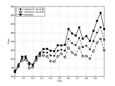
Figure 1: Price paths of the nontradable asset kerosene and the correlated asset heating oil at different correlation levels. The spot of kerosene was set to $r_{0}=170$.

We have seen that the valuation of the put option via utility maximization yields the pricing formula (8) which in conjunction with Lemma 3.1 becomes the difference of two solutions of a qgBSDE with the generator (10)

$$p_{t} =Y^{F}_{t}-Y^{0}_{t},\leavevmode\nobreak\ \leavevmode\nobreak\ 0\leq t\leq T,$$

where $F(x)=(K-x)^{+}$ for some strike $K>0$. For the numerical simulation of the qgFBSDE $Y^{F}$ and $Y^{0}$, we apply the exponential transformation to both BSDE (see Section 6) and then employ the algorithm by Bender and Denk (2007) with $N=100$ equidistant time points, $70000$ paths and a regression basis consisting of five monomials and the payoff function of the put option. The Picard iteration stops as soon as the difference of two subsequent time zero values is less than $10^{-5}$. Simulations reveal that $12$ to $13$ iterations are needed for solving one exponentially transformed qgFBSDE.

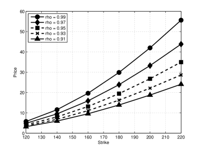
(a) Put option price in terms varying strikes at a fixed kerosene spot $r_{0}=170$.

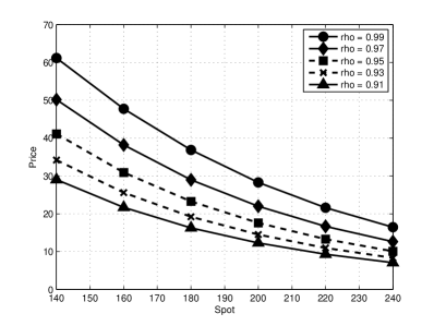
(b) Put option price in terms of varying kerosene spots at a fixed strike $K=200$.

Figure 2: Values of the put option in terms of kerosene spot and strike for varying correlations. High correlations lead to high the prices for the contingent claim.

Figures 2(a) and 2(b) depict the time zero price $p_{0}$ of the put option at different strike and kerosene spot levels. The lower the correlation, the lower the price becomes. This is clear because lower correlations between heating oil and kerosene lead to higher non-hedgeable residual risk which diminishes the risk covering effect of the contingent claim and thus also its value.

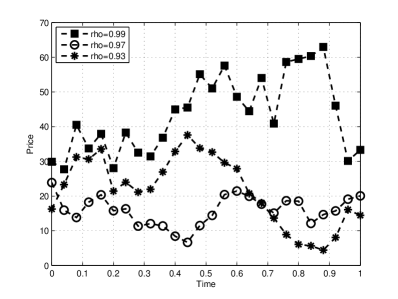
(a) Dynamics of the price process $p_{t}$ for strike $K=180$.

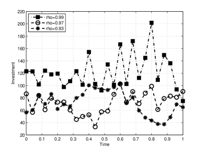
(b) Dynamics of the optimal investment strategy $\pi_{t}$ for strike $K=180$.

Figure 3: Paths of the price $p_{t}$ and the optimal investment strategy $\pi_{t}$ for varying correlation levels. In general high correlations entail greater market activity.

Figures 3(a) and 3(b) depict sample paths of the dynamics for the price $p_{t}$ and the optimal investment strategy $\pi_{t}$ for an at the money put with strike $K=180$ and kerosene spot $r_{0}=170$. The plots depict price and monetary investment for every fourth time point of the discretization. The price process and the dynamics of the optimal investment strategy are intertwined: high fluctuations of the price process result in high fluctuations of the investment strategy and vice versa. In general we observe that replication on high correlation levels tends to entail greater market activity because kerosene price risks can then be well hedged by market transactions that move closely along the dynamics of heating oil. In contrast, replication on lower correlation levels leads to a higher amount of residual risk which is inaccessible for hedging and thus lower market activity is needed.

Appendix 1 – Some results on BMO martingales

BMO martingales play a key role for a priori estimates needed in our sensitivity analysis of solutions of BSDE. For details about this theory we refer the reader to Kazamaki (1994).

Let $\Phi$ be a $BMO(\mathcal{F},\mathbb{Q})$ martingale with $\Phi_{0}=0$. $\Phi$ being square integrable, the martingale representation Theorem yields a square integrable process $\phi$ such that $\Phi_{t}=\int_{0}^{t}\phi_{s}\mathrm{d}W_{s},t\in[0,T]$. Hence the $BMO(\mathcal{F},\mathbb{Q})$ norm of $\Phi$ can be alternatively expressed as

$$\sup_{\tau\,\mathcal{F}-\mbox{\scriptsize stopping time in}\,[0,T]}\mathbb{E}^{\mathbb{Q}}\Big{[}\int_{\tau}^{T}\phi_{s}^{2}\mathrm{d}s|\mathcal{F}_{\tau}\Big{]}<\infty.$$

Lemma 7.1 (Properties of BMO martingales).

Let $\Phi$ be a $BMO$ martingale. Then we have:

• The stochastic exponential $\mathcal{E}(\Phi)$ is uniformly integrable.

• There exists a number $r>1$ such that $\mathcal{E}(\Phi_{T})\in L^{r}$. This property follows from the Reverse Hölder inequality. The maximal $r$ with this property can be expressed explicitly in terms of the BMO norm of $\Phi$.

• If $\Phi=\int_{0}^{\cdot}\phi_{s}\mathrm{d}s$ has BMO norm $C$, then for $p\geq 1$ the following estimate holds

  $$\mathbb{E}[\Big{(}\int_{0}^{T}|\phi_{s}|^{2}\mathrm{d}s\Big{)}^{p}]\leq 2p!(4C^{2})^{p}.$$

  Hence $BMO\subset\mathcal{H}^{p}$ for all $p\geq 1$.

Appendix 2 – Basics of Malliavin’s calculus

We briefly introduce the main notation of the stochastic calculus of variations also known as Malliavin’s calculus. For more details, we refer the reader to Nualart (2006). Let ${\bf\mathcal{S}}$ be the space of random variables of the form

$$\xi=F\Big{(}(\int_{0}^{T}h^{1,i}_{s}\mathrm{d}W^{1}_{s})_{1\leq i\leq n},\cdots,(\int_{0}^{T}h^{d,i}_{s}\mathrm{d}W^{d}_{s})_{1\leq i\leq n})\Big{)},$$

where $F\in C_{b}^{\infty}(\mathbb{R}^{n\times d})$, $h^{1},\cdots,h^{n}\in L^{2}([0,T];\mathbb{R}^{d})$, $n\in\mathbb{N}.$ To simplify notation, assume that all $h^{j}$ are written as row vectors. For $\xi\in{\bf\mathcal{S}}$, we define $D=(D^{1},\cdots,D^{d}):{\bf\mathcal{S}}\to L^{2}(\Omega\times[0,T])^{d}$ by

$$D^{i}_{\theta}\xi=\sum_{j=1}^{n}\frac{\partial F}{\partial x_{i,j}}\Big{(}\int_{0}^{T}h^{1}_{t}\mathrm{d}W_{t},\ldots,\int_{0}^{T}h^{n}_{t}\mathrm{d}W_{t}\Big{)}h^{i,j}_{\theta},\quad 0\leq\theta\leq T,\quad 1\leq i\leq d,$$

and for $k\in\mathbb{N}$ its $k$-fold iteration by

$$D^{(k)}=(D^{i_{1}}\cdots D^{i_{k}})_{1\leq i_{1},\cdots,i_{k}\leq d}.$$

For $k\in\mathbb{N},p\geq 1$ let $\mathbb{D}^{k,p}$ be the closure of $\mathcal{S}$ with respect to the norm

$$\lVert\xi\lVert_{k,p}^{p}=\mathbb{E}\Big{[}\|\xi\|^{p}_{L^{p}}+\sum_{i=1}^{k}\||D^{(k)]}\xi|\|_{(\mathcal{H}^{p})^{i}}^{p}\Big{]}.$$

$D^{(k)}$ is a closed linear operator on the space $\mathbb{D}^{k,p}$. Observe that if $\xi\in\mathbb{D}^{1,2}$ is $\mathcal{F}_{t}$-measurable then $D_{\theta}\xi=0$ for $\theta\in(t,T]$. Further denote $\mathbb{D}^{k,\infty}=\cap_{p>1}\mathbb{D}^{k,p}$.

We also need Malliavin’s calculus for smooth stochastic processes with values in $\mathbb{R}^{m}.$ For $k\in\mathbb{N},p\geq 1,$ denote by $\mathbb{L}_{k,p}(\mathbb{R}^{m})$ the set of $\mathbb{R}^{m}$-valued progressively measurable processes $u=(u^{1},\cdots,u^{m})$ on $[0,T]\times\Omega$ such that

• For Lebesgue-a.a. $t\in[0,T]$, $u(t,\cdot)\in(\mathbb{D}^{k,p})^{m}$;

• $[0,T]\times\Omega\ni(t,\omega)\mapsto D^{(k)}u(t,\omega)\in(L^{2}([0,T]^{1+k}))^{d\times n}$ admits a progressively measurable version;

• $\lVert u\lVert_{k,p}^{p}=\|u\|_{\mathcal{H}^{p}}^{p}+\sum_{i=1}^{k}\|\,D^{i}u\,\|_{(\mathcal{H}^{p})^{1+i}}^{p}\,<\infty$.

Note that Jensen’s inequality gives for all $p\geq 2$

$$\mathbb{E}\Big{[}\Big{(}\int_{0}^{T}\int_{0}^{T}|D_{u}X_{t}|^{2}\mathrm{d}u\,\mathrm{d}t\Big{)}^{\frac{p}{2}}\Big{]}\leq T^{p/2-1}\int_{0}^{T}\|D_{u}X\|_{\mathcal{H}^{p}}^{p}\mathrm{d}u.$$

Appendix 3 – Some results on SDE

We recall results on SDE known from the literature that are relevant for this work. We state our assumptions in the multidimensional setting. However, for ease of notation we present some formulas in the one dimensional case.

Theorem 7.2 (Moment estimates for SDE).

Assume that (H0) holds. Then (1) has a unique solution $X\in\mathcal{S}^{2}$ and the following moment estimates hold: for any $p\geq 2$ there exists a constant $C>0$, depending only on $T$, $K$ and $p$ such that for any $x\in\mathbb{R}^{m},s,t\in[0,T]$

$$\mathbb{E}[\,\sup_{0\leq t\leq T}|X_{t}|^{p}\,] \leq C\mathbb{E}\Big{[}\,|x|^{p}+\int_{0}^{T}\big{(}|b(t,0)|^{p}+|\sigma(t,0)|^{p}\big{)}\mathrm{d}t\Big{]},$$

$$\mathbb{E}[\sup_{s\leq u\leq t}|X_{u}-X_{s}|^{p}\,] \leq C\mathbb{E}\Big{[}\,|x|^{p}+\sup_{0\leq t\leq T}\big{\{}|b(t,0)|^{p}+|\sigma(t,0)|^{p}\big{\}}\Big{]}\,|t-s|^{p/2}.$$

Furthermore, given two different initial conditions $x,x^{\prime}\in\mathbb{R}^{m}$, we have

$$\mathbb{E}\Big{[}\sup_{0\leq t\leq T}|X_{t}^{x}-X_{t}^{x^{\prime}}|^{p}\Big{]}\leq C|x-x^{\prime}|^{p}.$$

Theorem 7.3 (Classical differentiability).

Assume (H1) holds. Then the solution process $X$ of (1) as a function of the initial condition $x\in\mathbb{R}^{m}$ is differentiable and satisfies for $t\in[0,T]$

$$\nabla X_{t} =I_{m}+\int_{0}^{t}\nabla b(X_{s})\nabla X_{s}\mathrm{d}s+\int_{0}^{t}\nabla\sigma(X_{s})\nabla X_{s}\mathrm{d}W_{s},$$ (21)

where $I_{m}$ denotes the $m\times m$ unit matrix. Moreover, $\nabla X_{t}$ as an $m\times m$-matrix is invertible for any $t\in[0,T]$. Its inverse $(\nabla X_{t})^{-1}$ satisfies an SDE and for any $p\geq 2$ there are positive constants $C_{p}$ and $c_{p}$ such that

$$\|\nabla X\|_{\mathcal{S}^{p}}+\|(\nabla X)^{-1}\|_{\mathcal{S}^{p}} \leq C_{p}$$

and

$$\mathbb{E}\Big{[}\sup_{s\leq u\leq t}|(\nabla X_{u})-(\nabla X_{s})|^{p}+\sup_{s\leq u\leq t}|(\nabla X_{u})^{-1}-(\nabla X_{s})^{-1}|^{p}\,\Big{]} \leq c_{p}\,|t-s|^{p/2}.$$

Theorem 7.4 (Malliavin Differentiability).

Under (H1), $X\in\mathbb{L}_{1,2}$ and its Malliavin derivative admits a version $(u,t)\mapsto D_{u}X_{t}$ satisfying for $0\leq u\leq t\leq T$ the SDE

$$D_{u}X_{t} =\sigma(X_{u})+\int_{u}^{t}\nabla b(X_{s})D_{u}X_{s}\mathrm{d}s+\int_{u}^{t}\nabla\sigma(X_{s})D_{u}X_{s}\mathrm{d}W_{s}.$$ (22)

Moreover, for any $p\geq 2$ there is a constant $C_{p}>0$ such that for $x\in\mathbb{R}^{m}$ and $0\leq v\leq u\leq t\leq s\leq T$

$$\|D_{u}X\|_{\mathcal{S}^{p}}^{p} \leq C_{p}(1+|x|^{p}),$$

$$\mathbb{E}[\,|D_{u}X_{t}-D_{u}X_{s}|^{p}] \leq C_{p}(1+|x|^{p})|t-s|^{\frac{p}{2}},$$

$$\|D_{u}X-D_{v}X\|_{\mathcal{S}^{p}}^{p} \leq C_{p}(1+|x|^{p})|u-v|^{\frac{p}{2}}.$$

By Theorem 7.3, we have the representation

$$D_{u}X_{t}=\nabla X_{t}(\nabla X_{u})^{-1}\sigma(X_{u})\textbf{1}_{[0,u]}(t),\quad\textrm{ for all }u,t\in[0,T].$$

Appendix 4 – Path regularity for Lipschitz FBSDE

We state a version of the $L^{2}$-regularity result for FBSDE satisfying a global Lipschitz condition. The result which was seen to be closely related to the convergence of numerical schemes for systems of FBSDE is due to Zhang (2001). For our FBSDE system (1), (2) we assume that $b,\sigma,f,g$ are deterministic measurable functions that are Lipschitz continuous with respect to the spatial variables and $\frac{1}{2}$-Hölder continuous with respect to time. Furthermore we assume that $\sigma$ satisfies (13). Then from El Karoui et al. (1997) one easily obtains existence and uniqueness of a solution triple $(X,Y,Z)$ of FBSDE (1), (2) belonging to $\mathcal{S}^{2}\times\mathcal{S}^{2}\times\mathcal{H}^{2}$. For a partition $\pi$ of $[0,T]$ define the process $\bar{Z}^{\pi}$ as in (15). Then the following result holds.

Theorem 7.5 (Path regularity result of Zhang (2001)).

Let $(X,Y,Z)\in\mathcal{S}^{2}\times\mathcal{S}^{2}\times\mathcal{H}^{2}$ be the solution of FBSDE (1), (2) in the setting described above. Then there exists $C\in\mathbb{R}_{+}$ such that for any partition $\pi=\{t_{0},\cdots,t_{N}\}$ of the time interval $[0,T]$ with mesh size $|\pi|$ we have

$$\max_{0\leq i\leq N-1}\Big{\{}\sup_{t\in[{t_{i}},{t_{i+1}})}\mathbb{E}\Big{[}\,|Y_{t}-Y_{t_{i}}|^{2}\Big{]}\Big{\}}$$

$$\qquad\quad+\sum_{i=0}^{N-1}\mathbb{E}\Big{[}\int_{t_{i}}^{t_{i+1}}|Z_{s}-\bar{Z}^{\pi}_{t_{i}}|^{2}\mathrm{d}s\Big{]}+\sum_{i=0}^{N-1}\mathbb{E}\Big{[}\int_{t_{i}}^{t_{i+1}}|Z_{s}-Z_{t_{i}}|^{2}\mathrm{d}s\Big{]}\leq C|\pi|.$$

References

• Ankirchner et al. (2007a) S. Ankirchner, P. Imkeller, and G. dos Reis. Pricing and hedging of derivatives based in non-tradable underlyings. To appear in Mathematical Finance, 2007a.
• Ankirchner et al. (2007b) S. Ankirchner, P. Imkeller, and G. dos Reis. Classical and variational differentiability of BSDEs with quadratic growth. Electron. J. Probab., 12(53):1418–1453 (electronic), 2007b.
• Bender and Denk (2007) C. Bender and R. Denk. A forward simulation of backward SDEs. Stochastic Process. Appl., 117(12):1793–1812, December 2007.
• Bouchard and Touzi (2004) B. Bouchard and N. Touzi. Discrete-time approximation and Monte-Carlo simulation of backward stochastic differential equations. Stochastic Process. Appl., 111(2):175–206, 2004.
• Briand and Confortola (2008) P. Briand and F. Confortola. BSDEs with stochastic Lipschitz condition and quadratic PDEs in Hilbert spaces. Stochastic Process. Appl., 118(5):818–838, 2008.
• Delarue and Menozzi (2006) F. Delarue and S. Menozzi. A forward-backward stochastic algorithm for quasi-linear PDEs. Ann. Appl. Probab., 16(1):140–184, 2006.
• dos Reis (2009) G. dos Reis. On some properties of solutions of quadratic growth BSDE and applications in finance and insurance. PhD thesis, Humboldt University, 2009.
• El Karoui et al. (1997) N. El Karoui, S. Peng, and M. C. Quenez. Backward stochastic differential equations in finance. Math. Finance, 7(1):1–71, 1997.
• Elie (2006) R. Elie. Contrôle stochastique et méthodes numériques en finance mathématique. PhD thesis, Université Paris-Dauphine, Décembre 2006.
• Frei (2009) C. Frei. Convergence results for the indifference value in a Brownian setting with variable correlation. Preprint, available at www.cmapx.polytechnique.fr/$\sim$frei, July 2009.
• Gobet et al. (2005) E. Gobet, J.-P. Lemor, and X. Warin. A regression-based Monte Carlo method to solve backward stochastic differential equations. Ann. Appl. Probab., 15(3):2172–2202, 2005.
• Imkeller et al. (2009) P. Imkeller, A. Réveillac, and A. Richter. Differentiability of quadratic BSDE generated by continuous martingales and hedging in incomplete markets. arXiv:0907.0941v1, June 2009.
• Kazamaki (1994) N. Kazamaki. Continuous exponential martingales and BMO, volume 1579 of Lecture Notes in Mathematics. Springer-Verlag, Berlin, 1994.
• Kobylanski (2000) M. Kobylanski. Backward stochastic differential equations and partial differential equations with quadratic growth. Ann. Probab., 28(2):558–602, 2000.
• Ma and Zhang (2002) J. Ma and J. Zhang. Path regularity for solutions of backward stochastic differential equations. Probab. Theory Related Fields, 122(2):163–190, 2002.
• Mania and Schweizer (2005) M. Mania and M. Schweizer. Dynamic exponential utility indifference valuation. Ann. Appl. Probab., 15(3):2113–2143, 2005.
• Morlais (2009) M.-A. Morlais. Quadratic BSDEs driven by a continuous martingale and applications to the utility maximization problem. Finance Stoch., 13(1):121–150, 2009.
• Nualart (2006) D. Nualart. The Malliavin calculus and related topics. Probability and its Applications (New York). Springer-Verlag, Berlin, second edition, 2006.
• Zhang (2001) J. Zhang. Some fine properties of BSDE. PhD thesis, Purdue University, August 2001.