Cholesteric order in systems of helical Yukawa rods

Abstract

We consider the interaction potential between two chiral rod-like colloids which consist of a thin cylindrical backbone decorated with a helical charge distribution on the cylinder surface. For sufficiently slender coiled rods a simple scaling expression is derived which links the chiral ‘twisting’ potential to the intrinsic properties of the particles such as the coil pitch, charge density and electrostatic screening parameter. To predict the behavior of the macroscopic cholesteric pitch we invoke a simple second-virial theory generalized for weakly twisted director fields. While the handedness of the cholesteric phase for weakly coiled rods is always commensurate with that of the internal coil, more strongly coiled rods display cholesteric order with opposite handedness. The correlation between the symmetry of the microscopic helix and the macroscopic cholesteric director field is quantified in detail. Mixing helices with sufficiently disparate lengths and coil pitches gives rise to a demixing of the uniform cholesteric phase into two fractions with a different macroscopic pitch. Our findings are consistent with experimental results and could be helpful in interpreting experimental observations in systems of cellulose and chitin microfibers, DNA and fd virus rods.

I Introduction

In contrast to a common nematic phase, where the nematic director is homogeneous throughout the system, the cholesteric (chiral nematic) phase is characterized by a helical arrangement of the director field along a common pitch axis. As a result, the cholesteric phase possesses an additional mesoscopic length scale, commonly referred to as the ‘cholesteric pitch ’, which characterizes the distance along the pitch axis over which the local director makes a full turn de Gennes and Prost (1993). The behavior of the pitch as a function of density, temperature and solvent conditions is of great fundamental and practical importance since the unique rheological, electrical and optical properties of cholesteric materials are determined in large part by the topology of the nematic director field.

In recent years considerable research effort has been devoted to studying chirality in lyotropic liquid crystals which consist of colloidal particles or stiff polymers immersed in a solvent. In addition to a number of synthetic helical polymers such as polyisocyanates Aharoni (1979); Sato et al. (1993) and polysilanes Watanabe et al. (2001) which form cholesteric phases in organic solvents there is a large class of helical bio-polymers which are known to form cholesteric phases in water. Examples are DNA Robinson (1961); Livolant and Leforestier (1996) and the rod-like $fd$-virus Dogic and Fraden (2006), polypeptides Uematsu and Uematsu (1984); DuPré and Samulski (1979), chiral micelles Hiltrop (2001), polysaccharides Sato and Teramoto (1996), and microfibrillar cellulose (and its derivatives) Werbowyj and Gray (1976) and chitin Revol and Marchessault (1993). In these systems, the cholesteric pitch is strongly dependent upon the particle concentration, temperature as well as e.g. the ionic strength which has been the subject of intense experimental research van Winkle et al. (1990); Yevdokimov et al. (1988); Stanley et al. (2005); Dogic and Fraden (2000); Grelet and Fraden (2003); Robinson (1961); DuPré and Duke (1975); Yoshiba et al. (2003); Dong and Gray (1997); Miller and Donald (2003); Dong et al. (1996).

Understanding the connection between the molecular interactions responsible for chirality on the microscopic scale and the structure of the macroscopic cholesteric phase has been a long-standing challenge in the physics of liquid crystals de Gennes and Prost (1993). The chiral nature of most biomacromolecules originates from a spatially non-uniform distribution of charges and dipole moments residing on the molecule. The most prominent example is the double-helix backbone structure of the phosphate groups in DNA. Combining the electrostatic interactions with the intrinsic conformation of the molecule allows for a coarse-grained description in terms of an effective chiral shape. Examples are bent-core or banana-shaped molecules Straley (1973); Jákli et al. (2007) where the mesogen shape is primarily responsible for chirality. Many other helical bio-polymers and microfibrillar assemblies of chiral molecules (such as cellulose) can be mapped onto effective chiral objects such as a threaded cylinder Straley (1973); Odijk (1987); Kimura et al. (1982), twisted rod Revol and Marchessault (1993); Orts et al. (1998) or semi-flexible helix Pelcovits (1996).

The construction of a microscopic theory for the cholesteric phase is a serious challenge owing to the complexity of the underlying chiral interaction and the inhomogeneous and anisotropic nature of the phase Harris et al. (1999). Course-grained model potentials aimed at capturing the essentials of the complex molecular nature of the electrostatics of the surface of such macromolecules have been devised mainly for DNA Strey et al. (1998); Kornyshev and Leikin (1997); Kornyshev and Leikin (2000); Kornyshev et al. (2002); Tombolato and Ferrarini (2005). A more general electrostatic model potential for chiral interactions was proposed much earlier by Goossens Goossens (1971) based on a spatial arrangement of dipole-dipole and dipole-quadrupole interactions which can be cast into a multipole expansion in terms of tractable pseudo-scalar potentials van der Meer and Vertogen (1979). This type of electrostatic description of the chiral interaction can be combined with a Maier-Saupe mean-field treatment van der Meer et al. (1976); Lin-Liu et al. (1977); Hu et al. (1998); Osipov and Kuball (2001); Kapanowski (2002); Emelyanenko (2003), or with a bare hard-core model and treated within the seminal theory of Onsager Onsager (1949); Varga and Jackson (2006); Wensink and Jackson (2009).

A drawback of the Goossens potential is that its simple scaling form precludes an explicit connection with the underlying microscopic (electrostatic) interactions involved. As a consequence, the potential is unsuitable for studying the sensitivity of the cholesteric pitch of charged rod-like colloids where the strength of the chiral interactions depends strongly on the configuration of the surface charges and the electrostatic screening (viz. salt concentration). In this paper, we propose a simple but explicit model for long-ranged chiral interactions based on an impenetrable cylindrical rod decorated with a helical coil of charges located on the rod surface. The local interactions between the charged helical segments is represented by a simple Yukawa potential in line with the Debye-Hückel approximation valid for weakly charged poly-electrolytes. A subsequent analysis of the chiral potential between a pair of helical Yukawa segment rods leads to a simple general expression which relates the intrinsic twisting potential to the electrostatic screening, charge density and coil pitch of the helices. The overall form of the chiral Yukawa potential resembles the one proposed by Goossens Goossens (1971), albeit with a much weaker decay with respect to the interrod distance. The most important difference, however, is that the amplitude of the chiral Yukawa potential can be linked to the coil configuration, and the local electrostatic potential. By mapping the helical charge distribution onto an effective helical coil the present model could be interpreted as a simple prototype for a charged twisted rod, a model commonly invoked to explain cholesteric organization of cellulose Orts et al. (1998); Yi et al. (2008) and chitin microfibers Revol and Marchessault (1993). Likewise, the $\alpha$-helical structure of polypeptide molecules Kimura et al. (1982) could also be conceived as a coiled rod on a coarse-grained level.

In the second part of the analysis, the potential will be employed in a simple Onsager second virial theory to predict the behavior of the macroscopic cholesteric pitch of Yukawa helices. The sensitivity of the pitch with respect to the coil configuration and amplitude of the electrostatic interactions will be scrutinized in detail. Also considered are the implications of mixing two helices species with different lengths and/or coil pitches on the isotropic-cholesteric phase behavior of mixed systems.

The theoretical results are consistent with experimental findings and correctly capture the response of the cholesteric pitch upon variation of the particle concentration and salt content. The theory also unveils a subtle relationship between the internal conformation (coil pitch) of the helical rod and the handedness of the cholesteric phase. The sensitive relationship between the symmetry of the cholesteric phase and the charge pattern on the rod surface is consistent with experimental observations in filamentous virus systems such as fd Barry et al. (2009) and M13 Tombolato et al. (2006) as well as numerical calculations based on a more explicit poly-electrolyte site model Tombolato et al. (2006).

This paper is structured as follows. In Section II we introduce the chiral Yukawa model and derive a general expression for the chiral potential imparted by the helical charge distribution. The implications of the potential for the macrosopic cholesteric pitch will be analyzed in detail in Section III where we shall focus first on monodisperse systems of identical helices followed by a treatment of binary mixtures of Yukawa helices differing in length and/or coil pitch. Finally, Section IV will be devoted to a discussion followed by some concluding remarks.

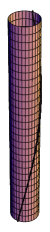
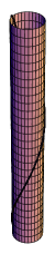
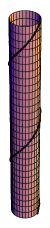
Figure 1: Cylinders decorated with a continuous helical charge distribution (indicated by the thread) with different coil pitches, $k=\pi$ (left), $k=2\pi$ (middle) and $k=4\pi$ (right).

II Chiral interaction between Yukawa helices

In this study we aim to quantify the chiral or twisting potential of a pair of charged helical colloidal rods starting from a continuum electrostatic model based on a screened Coulombic (or Yukawa) potential. Within linearized Poisson-Boltzmann theory the electrostatic interaction between two charged point particles with equal charge $\pm Ze$ in a dielectric solvent with relative permittivity $\varepsilon_{r}$ is given by Hansen and McDonald (2006):

$$\beta U_{Y}{(r)}=Z^{2}\lambda_{B}\frac{\exp[-\kappa r]}{r}$$ (1)

with $r$ the distance between the particles, $\lambda_{B}=e^{2}/4\pi\varepsilon_{0}\varepsilon_{r}k_{B}T$ the Bjerrum length ($\lambda_{B}=0.7$ $nm$ for water at $T=298K$), $\varepsilon_{0}$ the vacuum permittivity, and $\kappa$ the Debye screening constant $\kappa=\sqrt{4\pi\lambda_{B}(Z\rho+2c_{s})}$ which measures the extent of the electric double layer surrounding each particle. Here, $\rho=N/V$ is the macro-ion density, $N_{av}$ is Avogadro’s number, and $c_{s}$ refers to the concentration of added salt.

Eq. (1) can be generalized in a straightforward manner to describe the interaction between two helical macro-ions by assuming that the total pair potential can be written as a summation over Yukawa sites residing on the helices (see Fig. 1). In the limit of an infinite number of sites per unit length the electrostatic potential of helical rods with variable lengths $L_{1}$ and $L_{2}$, and common diameter $D$ at positions $\{{\bf r}_{1}$ ,${\bf r}_{2}\}$ and orientational unit vectors $\{{\bf\hat{u}}_{1}$ ${\bf\hat{u}}_{2}\}$ is then given by a double contour integral over the longitudinal (pitch) axes of the helices:

$$\beta U_{Y}(\Delta{\bf r};{\bf\hat{u}}_{1},{\bf\hat{u}}_{2};\psi_{1},\psi_{2}) = Z_{1}Z_{2}\lambda_{B}\int_{-1}^{1}dt_{1}\int_{-1}^{1}dt_{2}$$ (2)

$$\times\frac{\exp[-\kappa|{\bf r}_{2}^{s}-{\bf r}_{1}^{s}|]}{|{\bf r}_{2}^{s}-{\bf r}_{1}^{s}|}$$

with $\Delta{\bf r}={\bf r}_{2}-{\bf r}_{1}$ the distance vector between the centre-of-masses of the helices, and $Z_{i}$ is the total number of charges on species $i$.

In order to describe the segment position ${\bf r}_{i}^{s}$ along the contour of helix $i$ it is expedient to introduce a particle-based Cartesian frame spanned by tree orthogonal unit vectors $\{{\bf\hat{u}}_{i},{\bf\hat{v}},{\bf\hat{w}}_{i}\}$ $(i=1,2)$, where ${\bf\hat{v}}={\bf\hat{u}}_{1}\times{\bf\hat{u}}_{2}/|{\bf\hat{u}}_{1}\times{\bf\hat{u}}_{2}|$ and ${\bf\hat{w}}_{i}={\bf\hat{u}}_{i}\times{\bf\hat{v}}$. Within the particle the segment positions can be parametrized as follows:

$${\bf r}_{1}^{s} = {\bf r}_{1}+\frac{L_{1}}{2}t_{1}{\bf\hat{u}}_{1}+\frac{D}{2}$$

$$\times\left\{\cos(k_{1}t_{1}+\psi_{1}){\bf\hat{v}}+\sin(k_{1}t_{1}+\psi_{1}){\bf\hat{w}}_{1}\right\}$$

$${\bf r}_{2}^{s} = {\bf r}_{2}+\frac{L_{2}}{2}t_{2}{\bf\hat{u}}_{2}+\frac{D}{2}$$ (3)

$$\times\left\{\cos(k_{2}t_{2}+\psi_{2}){\bf\hat{v}}+\sin(k_{2}t_{2}+\psi_{2}){\bf\hat{w}}_{2}\right\}$$

in terms of the dimensionless contour variables $t_{i}$ ($-1\leq t_{i}\leq 1$) and coil pitch $k_{i}=2\pi L_{i}/p_{\text{int}}^{(i)}$ with $p_{\text{int}}^{(i)}$ the distance along the longitudinal rod axis over which the Yukawa helix makes a full revolution. With this convention $k_{i}>0$ corresponds to a right-handed helix and $k_{i}<0$ to a left-handed one.

In this study we will focus on the general case of a binary mixture of helical species with a different coil pitch (in terms of sign and/or magnitude), i.e. $k_{1}\neq k_{2}$. Since a helix is not invariant with respect to rotations about the longitudinal pitch axis ${\bf\hat{u}}_{i}$ we need to define an additional orientational unit vector ${\bf\hat{e}}_{i}\perp{\bf\hat{u}}_{i}$ to account for its azimuthal degress of freedom. Consequently, the interaction potential Eq. (2) must depend on a set of internal azimuthal angles $\psi_{i}$ ($0\leq\psi_{i}\leq 2\pi$), defined such that $\cos\psi_{i}={\bf\hat{w}}_{i}\cdot{\bf\hat{e}}_{i}$. Using Eq. (3) and employing orthogonality of the unit vectors allows us to derive an expression for the norm of the segment-segment distance. Let us normalize the centre-of-mass distance in units of rod length of species 1, $L_{1}$, so that $\Delta{\bf r}\rightarrow\Delta{\bf r}/L_{1}$. If we further assume the helices to be sufficiently slender ($D/L_{i}\ll 1$) we may Taylor expand the potential up to leading order in $D/L_{i}$:

$$\beta U_{Y}(\Delta{\bf r};{\bf\hat{u}}_{1},{\bf\hat{u}}_{2};\psi_{1},\psi_{2}) \simeq \beta U_{Y}^{(0)}(\Delta{\bf r};{\bf\hat{u}}_{1},{\bf\hat{u}}_{2})-Z_{1}Z_{2}\left(\frac{\lambda_{B}}{D}\right)\left(\frac{D}{L_{1}}\right)^{2}\int_{-1}^{1}dt_{1}\int_{-1}^{1}dt_{2}U^{\prime}_{Y}(\Delta\tilde{r})$$ (4)

$$\times\left\{\left[\cos(k_{2}t_{2}+\psi_{2})-\cos(k_{1}t_{1}+\psi_{1})\right]({\bf\hat{v}}\cdot\Delta{\bf r})\right.$$

$$+\left[\sin(k_{2}t_{2}+\psi_{2})({\bf\hat{w}}_{2}\cdot\Delta{\bf r})-\sin(k_{1}t_{1}+\psi_{1})({\bf\hat{w}}_{1}\cdot\Delta{\bf r})\right]$$

$$\left.-(1/2)\left[t_{1}\sin(k_{2}t_{2}+\psi_{2})({\bf\hat{w}}_{2}\cdot{\bf\hat{u}}_{1})+\ell t_{2}\sin(k_{1}t_{1}+\psi_{1})({\bf\hat{w}}_{1}\cdot{\bf\hat{u}}_{2})\right]\right\}+{\cal O}[(D/L)^{2}]$$

in terms of the length ratio $\ell=L_{2}/L_{1}$ and $U^{\prime}_{Y}$ the derivative of the Yukawa potential with respect to distance:

$$U^{\prime}_{Y}(\Delta\tilde{r})=\frac{\exp[-\kappa L_{1}\Delta\tilde{r}]}{2\Delta\tilde{r}}\left(\frac{\kappa L_{1}}{\Delta\tilde{r}}+\frac{1}{\Delta\tilde{r}^{2}}\right)$$ (5)

and $\Delta\tilde{r}$ the distance between the positions $t_{1}$ and $t_{2}$ along the pitch axis of the helices (in units $L_{1}$):

$$\Delta\tilde{r}^{2} = \Delta r^{2}+\left[\ell t_{2}({\bf\hat{u}}_{2}\cdot\Delta{\bf r})-t_{1}({\bf\hat{u}}_{1}\cdot\Delta{\bf r})\right]$$ (6)

$$+\frac{1}{4}[t_{1}^{2}+\ell^{2}t_{2}^{2}-2\ell t_{1}t_{2}({\bf\hat{u}}_{1}\cdot{\bf\hat{u}}_{2})]$$

The reference potential $\beta U_{Y}$ in Eq. (4) represents the pair potential between two screened line charges of length $L_{1}$ and $L_{2}$ interacting via the Yukawa potential Kirchhoff et al. (1996):

$$\beta U_{Y}^{(0)}(\Delta{\bf r};{\bf\hat{u}}_{1},{\bf\hat{u}}_{2}) = Z_{1}Z_{2}\left(\frac{\lambda_{B}}{D}\right)\left(\frac{D}{L_{1}}\right)\int_{-1}^{1}dt_{1}\int_{-1}^{1}dt_{2}$$ (7)

$$\times\frac{\exp[-\kappa L_{1}\Delta\tilde{r}]}{\Delta\tilde{r}}$$

Since this potential is strictly achiral we will disregard it in the sequel of this paper. Focusing now on the second, chiral contribution in Eq. (4) and applying standard trigonometric manipulations we may recast it into the following form:

$$\beta U_{Y}^{(c)}(\Delta{\bf r};{\bf\hat{u}}_{1},{\bf\hat{u}}_{2};\psi_{1},\psi_{2})=$$

$$-Z_{1}Z_{2}\left(\frac{\lambda_{B}}{D}\right)\left(\frac{D}{L_{1}}\right)^{2}\int_{-1}^{1}dt_{1}\int_{-1}^{1}dt_{2}U^{\prime}_{Y}(\Delta\tilde{r})$$

$$\times\left\{{\cal A}\cos\psi_{1}+{\cal B}\cos\psi_{2}+{\cal C}\sin\psi_{1}+{\cal D}\sin\psi_{2}\right\}$$ (8)

Henceforth, we will denote this potential by superscript “$c$”. The coefficients are given by:

$${\cal A} = -\cos(k_{1}t_{1})({\bf\hat{v}}\cdot\Delta{\bf r})-\sin(k_{1}t_{1})({\bf\hat{w}}_{1}\cdot\Delta{\bf r})$$

$$-\frac{\ell t_{2}}{2}\sin(k_{1}t_{1})({\bf\hat{w}}_{1}\cdot{\bf\hat{u}}_{2})$$

$${\cal B} = \cos(k_{2}t_{2})({\bf\hat{v}}\cdot\Delta{\bf r})+\sin(k_{2}t_{2})({\bf\hat{w}}_{2}\cdot\Delta{\bf r})$$

$$-\frac{t_{1}}{2}\sin(k_{2}t_{2})({\bf\hat{w}}_{2}\cdot{\bf\hat{u}}_{1})$$

$${\cal C} = \sin(k_{1}t_{1})({\bf\hat{v}}\cdot\Delta{\bf r})-\cos(k_{1}t_{1})({\bf\hat{w}}_{1}\cdot\Delta{\bf r})$$

$$-\frac{\ell t_{2}}{2}\cos(k_{1}t_{1})({\bf\hat{w}}_{1}\cdot{\bf\hat{u}}_{2})$$

$${\cal D} = -\sin(k_{2}t_{2})({\bf\hat{v}}\cdot\Delta{\bf r})+\cos(k_{2}t_{2})({\bf\hat{w}}_{2}\cdot\Delta{\bf r})$$ (9)

$$-\frac{t_{1}}{2}\cos(k_{2}t_{2})({\bf\hat{w}}_{2}\cdot{\bf\hat{u}}_{1})$$

The next step is to construct an angle-averaged potential $\beta{\bar{U}_{Y}^{(c)}}$ by carrying out a proper preaveraging over the internal azimuthal angles. By requiring the Helmholtz free energy of the angle-averaged potential to be equal to that of the full angle-dependent potential one can show that Israelachvili (1991):

$$\beta{\bar{U}_{Y}^{(c)}} = -\ln\left\langle\exp[-\beta U_{Y}^{(c)}]\right\rangle_{\psi_{1,2}}=\left\langle\beta U_{Y}^{(c)}\right\rangle_{\psi_{1,2}}$$

$$-\frac{1}{2}\left(\left\langle(\beta U_{Y}^{(c)})^{2}\right\rangle_{\psi_{1,2}}-\left\langle\beta U_{Y}^{(c)}\right\rangle_{\psi_{1,2}}^{2}\right)+\cdots$$

where the brackets denote a double integral over the internal angles $\langle.\rangle_{\psi}=(2\pi)^{-1}\int_{0}^{2\pi}d\psi$. A similar expression can be obtained starting from a self-consistent Boltzmann-weighted average of the chiral potential, i.e $\bar{U}=\langle U\exp[-\beta U]\rangle_{\psi_{1,2}}/\langle\exp[-\beta U]\rangle_{\psi_{1,2}}$ and Taylor expanding for small $\beta U$. This will give the same result except for a trivial prefactor in the fluctuation term Rushbrooke (1940); Rowlinson (1958). The leading order contribution $\langle\beta U_{Y}^{(c)}\rangle_{\psi_{1,2}}$ vanishes Tombolato and Ferrarini (2005) upon integrating over $\psi_{i}$ so that we need to consider the next-order fluctuation term in Eq. (II). Using the isotropic averages $\langle\cos^{2}\psi\rangle_{\psi}=\langle\sin^{2}\psi\rangle_{\psi}=1/2$ the angle-averaged chiral potential becomes:

$$\beta\bar{U}_{Y}^{(c)}(\Delta{\bf r};{\bf\hat{u}}_{1},{\bf\hat{u}}_{2}) \simeq -\frac{1}{4}Z_{1}^{2}Z_{2}^{2}\left(\frac{\lambda_{B}}{D}\right)^{2}\left(\frac{D}{L_{1}}\right)^{4}$$ (11)

$$\times\left({\cal\tilde{A}}^{2}+{\cal\tilde{B}}^{2}+{\cal\tilde{C}}^{2}+{\cal\tilde{D}}^{2}\right)$$

where

$${\cal\tilde{A}}=\int_{-1}^{1}dt_{1}\int_{-1}^{1}dt_{2}U^{\prime}_{Y}(\Delta\tilde{r}){\cal A}$$ (12)

and identical relations for the other coefficients. A close inspection of the coefficients Eq. (9) reveals that only those terms proportional to the pseudo-scalar ${\bf\hat{v}}\cdot\Delta{\bf r}$ contribute to the chiral potential. These are given by products involving the first and third terms in Eq. (9). All other contributions are invariant under a parity transformation $\Delta{\bf r}\rightarrow-\Delta{\bf r}$ which renders them irrelevant for the present analysis. If we use the standard representation for the triple product ${\bf\hat{u}}_{1}\times({\bf\hat{u}}_{1}\times{\bf\hat{u}}_{2})={\bf\hat{u}}_{1}({\bf\hat{u}}_{1}\cdot{\bf\hat{u}}_{2})-{\bf\hat{u}}_{2}({\bf\hat{u}}_{1}\cdot{\bf\hat{u}}_{1})$ so that $-{\bf\hat{w}}_{1}\cdot{\bf\hat{u}}_{2}={\bf\hat{w}}_{2}\cdot{\bf\hat{u}}_{1}=\sin\gamma$ (with $\gamma$ the angle between the main axes of the helices) the chiral potential simplifies to:

$$\beta\bar{U}_{Y}^{(c)}(\Delta{\bf r};{\bf\hat{u}}_{1},{\bf\hat{u}}_{2}) \simeq -\frac{1}{8}Z_{1}^{2}Z_{2}^{2}\left(\frac{\lambda_{B}}{L_{1}}\right)^{2}\left(\frac{D}{L_{1}}\right)^{2}$$ (13)

$$\times{\cal F}_{12}(\Delta r;k_{1},k_{2})\chi$$

in terms of a pseudo-scalar $\chi$ which changes sign under a parity transformation van der Meer and Vertogen (1979) $\Delta{\bf r}\rightarrow-\Delta{\bf r}$:

$$\chi=({\bf\hat{u}}_{1}\times{\bf\hat{u}}_{2}\cdot\Delta\hat{{\bf r}})$$ (14)

with $\Delta\hat{{\bf r}}=\Delta{\bf r}/|\Delta{\bf r}|$ the centre-of-mass unit vector. The function ${\cal F}_{12}$ depends on the distance and helix orientations and is invariant under parity transformation:

$${\cal F}_{12}(\Delta r;k_{1},k_{2}) = -\langle\cos(k_{1}t_{1})\rangle_{t_{1,2}}\langle\ell t_{2}\sin(k_{1}t_{1})\rangle_{t_{1,2}}$$ (15)

$$-\langle\cos(k_{2}t_{2})\rangle_{t_{1,2}}\langle t_{1}\sin(k_{2}t_{2})\rangle_{t_{1,2}}$$

$$+\langle\sin(k_{1}t_{1})\rangle_{t_{1,2}}\langle\ell t_{2}\cos(k_{1}t_{1})\rangle_{t_{1,2}}$$

$$+\langle\sin(k_{2}t_{2})\rangle_{t_{1,2}}\langle t_{1}\cos(k_{2}t_{2})\rangle_{t_{1,2}}$$

where the brackets are short-hand notation for the double contour integration over $\beta U_{Y}^{\prime}$:

$$\langle.\rangle_{t_{1,2}}=\Delta r^{1/2}\int_{-1}^{1}dt_{1}\int_{-1}^{1}dt_{2}U_{Y}^{\prime}(\Delta\tilde{r})$$ (16)

Since the prefactor ${\cal F}_{12}$ depends rather intricately on the centre-of-mass distance and orientations it is desirable to seek a simplified form. This can be achieved by ignoring the interactions involving the ends of the helix. Indeed, if we take the limit of $L_{i}/D\rightarrow\infty$ the second contribution in Eq. (6), which embodies the interaction between the end of one rod with the main section of the other, becomes vanishingly small. An equivalent approach would be to fix the centre-of-mass distance vector along the unit vector $\Delta{\bf r}=\Delta r{\bf\hat{v}}$. In either case, the segment-segment distance Eq. (6) simplifies to:

$$\Delta\tilde{r}^{2}\simeq\Delta r^{2}+\frac{1}{4}(t_{1}^{2}+\ell^{2}t_{2}^{2}-2\ell t_{1}t_{2}\cos\gamma)$$ (17)

and the only angular dependence is contained in the angle $\gamma$ between the main axes of the helices. The $\gamma$-dependence of the chiral potential at fixed centre-of-mass distance has been plotted in Fig. 2 and reveals a strongly non-monotonic relation. In a concentrated cholesteric nematic phase rods are usually strongly aligned along the local director so that $\gamma$ will on average be very small. In the asymptotic limit of strong local orientational order the following scaling expression for the chiral potential can be justified:

$$\beta\bar{U}_{Y}^{(c)}\propto\gamma{\cal F}_{12}(\Delta r;k_{1},k_{2})({\bf\hat{v}}\cdot\Delta\hat{{\bf r}})$$ (18)

where $\Delta\tilde{r}=[\Delta r^{2}+\frac{1}{4}(t_{1}-\ell t_{2})^{2}]^{1/2}$. Looking at the local minima appearing in Fig. 2 it is obvious that the asymptotic approximation has to be taken with some caution in the dilute regime where the average $\gamma$ is no longer very small. A striking anomaly occurs for $k=4$ where the chiral torque $(\partial U_{Y}^{(c)}/\partial\gamma)_{\gamma=0}$ has an opposite sign compared to the other cases shown. Moreover, the local and global minimum occurring for $k=4$ correspond to opposite twist directions. This hints to a subtle relationship between the magnitude of the coil pitch and the sense of the cholesteric director field which will be explored in detail further on in this study. In the asymptotic approximation, the distance dependence of the chiral potential is embodied by the chiral amplitude ${\cal F}_{12}$ which will be analyzed in the subsequent paragraphs where we will focus on identical and enantiomeric helices, respectively.

II.1 Identical helices

If the helices are identical, then $L_{1}=L_{2}=L$ ($\ell=1$), $k_{1}=k_{2}=k$ and $Z_{1}=Z_{2}=Z$. The double contour integration Eq. (16) is invariant under interchanging $t_{1}\leftrightarrow t_{2}$ and we can exploit this symmetry to simplify Eq. (15) as follows:

$${\cal F}(\Delta r;k) = -2\langle\cos(kt_{1})\rangle_{t_{1,2}}\langle t_{2}\sin(kt_{1})\rangle_{t_{1,2}}$$ (19)

$$+2\langle\sin(kt_{1})\rangle_{t_{1,2}}\langle t_{2}\cos(kt_{1})\rangle_{t_{1,2}}$$

The second contribution involves odd terms in $t_{1}$ and $t_{2}$ which vanish upon performing the double contour integration [Eq. (16)]. The result is:

$${\cal F}(\Delta r;k) = -2\Delta r\left(\int_{-1}^{1}dt_{1}\int_{-1}^{1}dt_{2}U_{Y}^{\prime}(\Delta\tilde{r})\cos(kt_{1})\right)$$ (20)

$$\times\left(\int_{-1}^{1}dt_{1}\int_{-1}^{1}dt_{2}U_{Y}^{\prime}(\Delta\tilde{r})t_{2}\sin(kt_{1})\right)$$

which still implicitly depends on the coil pitch $k$ and Debye screening length $\kappa L$ via Eq. (5). The chiral potential between two identical helical Yukawa rods thus reads:

$$\beta\bar{U}_{Y}^{(c)}(\Delta{\bf r};{\bf\hat{u}}_{1},{\bf\hat{u}}_{2})\simeq-\frac{1}{8}Z^{4}\left(\frac{\lambda_{B}}{D}\right)^{2}\left(\frac{D}{L}\right)^{4}{\cal F}(\Delta r;k)\chi$$ (21)

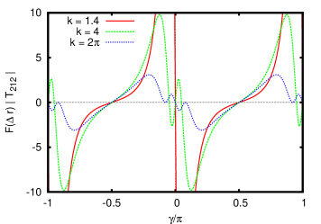
Figure 2: Reduced chiral potential ${\mathcal{F}}(\Delta r)|\chi|$ between two helical Yukawa rods as a function of the interrod angle $\gamma$ for fixed centre-of-mass distance $\Delta r=0.1L$ and $\kappa L=20$.

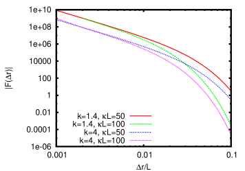
Figure 3: Amplitude of the chiral potential [Eq. (20)] between two helical Yukawa rods as a function of centre-of-mass distance $\Delta r=\Delta{\bf r}\cdot{\bf\hat{v}}$.

This potential, shown in Fig. 3, is found to decay steeply with increasing rod centre-of-mass distance. Owing to the intractable double contour integrations, the distance-dependence of the potential is essentially non-algebraic and does not obey a simple power-law scaling with respect to $\Delta r$. At short distances the amplitudes appear to be mainly dependent upon the coil pitch $k$ rather than the screening constant.

It is worthwhile to compare the chiral potential Eq. (21) to the one proposed by Goossens Goossens (1971); Wensink and Jackson (2009) which has been used frequently in literature. The Goossens potential emerges as the leading order contribution from a multipolar expansion of the interaction potential between two molecules each composed of an array of dipoles. This potential takes the following generic form:

$$U_{GS}(\Delta{\bf r};{\bf\hat{u}}_{1},{\bf\hat{u}}_{2})=-U_{0}\left(\frac{\sigma}{\Delta r}\right)^{7}({\bf\hat{u}}_{1}\cdot{\bf\hat{u}}_{2})\chi$$ (22)

in terms of a reference size $\sigma$ and amplitude $U_{0}$ which determines the handedness of the chiral interaction. As can be gleaned from Fig. 3 the distance-dependence of the Goossens potential is much steeper compared to the decay found from Eq. (20). We further remark that both chiral potentials are invariant with respect to an inversion of the rod orientation (${\bf\hat{u}}_{i}\rightarrow-{\bf\hat{u}}_{i}$, or equivalently $\gamma\rightarrow\gamma\pm\pi$).

II.2 Enantiomers: helices with opposite handedness

Let us now consider two helices of identical length $L_{1}=L_{2}=L$ and charge $Z_{1}=Z_{2}=Z$ but opposite pitch $k_{1}=-k_{2}$. The corresponding cross interaction between a right-handed and left-handed helix then follows from Eq. (15):

$${\cal F}_{12}(\Delta r;k_{1},-k_{1}) = -\langle\cos(k_{1}t_{1})\rangle_{t_{1,2}}\langle t_{2}\sin(k_{1}t_{1})\rangle_{t_{1,2}}$$ (23)

$$-\langle\cos(-k_{1}t_{2})\rangle_{t_{1,2}}\langle t_{1}\sin(-k_{1}t_{2})\rangle_{t_{1,2}}$$

$$+\langle\sin(k_{1}t_{1})\rangle_{t_{1,2}}\langle t_{2}\cos(k_{1}t_{1})\rangle_{t_{1,2}}$$

$$+\langle\sin(-k_{1}t_{2})\rangle_{t_{1,2}}\langle t_{1}\cos(-k_{1}t_{2})\rangle_{t_{1,2}}$$

$$= 0$$

irrespective of the magnitude of the coil pitch. The implication of this result is that an equimolar binary mixture of helices with equal shape but opposite handedness (a so-called ‘racemic’ mixture) does not exhibit cholesteric nematic order. If the rods have different lengths ($\ell\neq 1$) they no longer form an enantiomeric pair and the chiral interaction will generally be non-zero.

III Prediction of the cholesteric pitch

In order to study the implications of the internal helical structure of the rods on the (macroscopic) cholesteric order we need a statistical theory which is able to make a connection between the pair interaction of the particles and the local equilibrium orientational distribution $f({\bf\hat{u}}\cdot{\bf\hat{n}})$ and cholesteric pitch. Such a theory can be devised starting from the classical Onsager theory Onsager (1949) for infinitely thin hard rods which exhibit common uniaxial nematic order. The theory has been generalized by Straley Straley (1976); Allen et al. (1993) for aligned fluids with weakly non-uniform director fields, such as a cholesteric liquid crystal, in which case elastic contributions must be incorporated into the free energy. The Helmholtz free energy density $F/V$ of a binary mixture of slender chiral rods in a cholesteric phase of volume $V$ takes the following form:

$$\frac{\beta F}{V} = \rho(\ln\rho{\mathcal{\bar{V}}}-1)+\rho\sum_{i}x_{i}\int d{\bf\hat{u}}f_{i}({\bf\hat{u}})\ln[x_{i}4\pi f_{i}({\bf\hat{u}})]$$ (24)

$$+\beta\sum_{i}\sum_{j}x_{i}x_{j}\left(K_{0}^{ij}-K_{1}^{ij}q+\frac{K_{2}^{ij}}{2}q^{2}\right)$$

In terms of the thermal energy $\beta^{-1}=k_{B}T$, overall particle density $\rho=N/V$. ${\mathcal{\bar{V}}}=\prod_{i}{\mathcal{V}}^{x_{i}}$ is a weighted product of the thermal volume ${\mathcal{V}}_{i}$ of particle $i$ which includes contributions arising from the rotational momenta. The first two terms in the free energy denote the ideal translational and orientational entropy of the system while the last one represents the excess free energy which accounts for the interactions between the rods on the approximate second-virial level. The latter consists of three contributions. The first, $K_{0}$, involves a spatial and orientational average of the Mayer function $f_{M}=\exp[-\beta U]-1$ weighted by the orientational distribution functions (ODF) $f_{i}({\bf\hat{u}})$ of the respective species:

$$\beta K_{0}^{ij} = -\frac{\rho^{2}}{2}\int d{\bf\hat{u}}_{1}f_{i}({\bf\hat{u}}_{1})\int d{\bf\hat{u}}_{2}f_{j}({\bf\hat{u}}_{2})$$ (25)

$$\times\int d\Delta{\bf r}f^{ij}_{M}(\Delta{\bf r};{\bf\hat{u}}_{1},{\bf\hat{u}}_{2})$$

For hard anisometric bodies, the spatial integration leads to the excluded volume $v_{\text{excl}}^{ij}({\bf\hat{u}}_{1},{\bf\hat{u}}_{2})$ between particles of species $i$ and $j$. The second and third contributions in the excess free energy represent the change of free energy due to the twist deformation of the director field. The strength of this deformation is measured by the cholesteric pitch $q=2\pi/p$, with $p\gg L\gg p_{\text{int}}$ the pitch distance associated with the helical director field. Since the theory is only valid for long-wavelength distortions of the director field it is required that $q\ll 1$. The torque-field contribution, proportional to $K^{ij}_{1}q$ arises from the chiral torque imparted by the chirality of the particles and leads to a reduction of the free energy. Opposing this, there is an elastic response counteracting the deformation of the director field. The corresponding free energy penalty $K^{ij}_{2}q^{2}$ is proportional to the twist elastic constant $K_{2}^{ij}$. Similar to $K_{0}$, the torque-field and twist elastic constants are given by spatio-angular averages of the Mayer function, albeit in a more complicated way Allen et al. (1993):

$$\beta K_{1}^{ij} = -\frac{\rho^{2}}{2}\int d{\bf\hat{u}}_{1}f_{i}({\bf\hat{u}}_{1})\int d{\bf\hat{u}}_{2}\dot{f}_{j}({\bf\hat{u}}_{2})({\bf\hat{u}}_{2}\cdot{\bf\hat{y}})$$

$$\times\int d\Delta{\bf r}(\Delta z)f^{ij}_{M}(\Delta{\bf r};{\bf\hat{u}}_{1},{\bf\hat{u}}_{2})$$

$$\beta K_{2}^{ij} = -\frac{\rho^{2}}{2}\int d{\bf\hat{u}}_{1}\dot{f}_{i}({\bf\hat{u}}_{1})({\bf\hat{u}}_{1}\cdot{\bf\hat{y}})\int d{\bf\hat{u}}_{2}\dot{f}_{j}({\bf\hat{u}}_{2})({\bf\hat{u}}_{2}\cdot{\bf\hat{y}})$$ (26)

$$\times\int d\Delta{\bf r}(\Delta z)^{2}f^{ij}_{M}(\Delta{\bf r};{\bf\hat{u}}_{1},{\bf\hat{u}}_{2})$$

where $\dot{f}$ represents the derivative of the ODF with respect to its argument. In arriving at Eq. (26) we have implicitly fixed the pitch direction along the $z$-direction of the laboratory frame with the local nematic director ${\bf\hat{n}}(z)$ pointing parallel to the $x$-axis.

Let us now consider a model binary mixture of hard rods with different lengths ($\ell\neq 1$) decorated with a weak chiral potential of the form proposed in the previous section [Eq. (13)]. The twist elastic constant is not affected by the weak chiral potential, but only by the achiral hard cylindrical backbone and electrostatic reference potential. If we neglect the latter contributions for the time being the spatial integrals appearing in Eq. (25) and Eq. (26) reduce to integrals over the excluded volume manifold of two thin hard cylinders weighted over powers of the pitch distance variable $\Delta z$:

$$M_{n}^{ij}({\bf\hat{u}}_{1},{\bf\hat{u}}_{2})=\int_{\in v^{ij}_{\text{excl}}}\Delta{\bf r}(\Delta z)^{n},\hskip 14.22636ptn=0,2$$ (27)

These quantities have been calculated in general form for hard spherocylinders in Ref. Wensink and Jackson, 2009. Here, we only need the leading order contributions for large $L_{i}/D$:

$$M^{ij}_{0}({\bf\hat{u}}_{1},{\bf\hat{u}}_{2}) = v^{ij}_{\text{excl}}({\bf\hat{u}}_{1},{\bf\hat{u}}_{2})=2L_{i}L_{j}D|\sin\gamma|$$

$$M^{ij}_{2}({\bf\hat{u}}_{1},{\bf\hat{u}}_{2}) = \frac{2}{3}L_{i}L_{j}D|\sin\gamma|\left(\frac{L_{i}^{2}}{4}({\bf\hat{u}}_{1}\cdot{\bf\hat{z}})^{2}\right.$$ (28)

$$\left.+\frac{L_{j}^{2}}{4}({\bf\hat{u}}_{2}\cdot{\bf\hat{z}})^{2}+D^{2}({\bf\hat{v}}\cdot{\bf\hat{z}})^{2}\right)$$

Due to symmetry reasons the torque-field constant $K_{1}$ depends only the chiral part of the potential and not on the achiral reference part. For weak chiral potentials considered here it is justified to approximate $f_{M}\approx-\beta U$, analogous to a van der Waals perturbation approximation generalized to liquid crystals Gelbart and Baron (1977); Franco-Melgar et al. (2008); Wensink and Jackson (2009). The spatial integration pertaining to $M_{1}$ then becomes:

$$M_{1}^{ij}({\bf\hat{u}}_{1},{\bf\hat{u}}_{2})=\int_{\notin v^{ij}_{\text{excl}}}\Delta{\bf r}(\Delta z)\beta{\bar{U}}_{Y}^{(c)}(\Delta{\bf r};{\bf\hat{u}}_{1},{\bf\hat{u}}_{2})$$ (29)

where the spatial integral runs over the space complementary to the excluded volume of the particles. By exploiting the cylindrical symmetry of the cholesteric system one can parametrize the distance vector in terms of cylindrical coordinates so that $\Delta{\bf r}=r\sin\zeta{\bf\hat{x}}+r\cos\zeta{\bf\hat{y}}+\Delta z{\bf\hat{z}}$. With this, one can write :

$$M_{1}^{ij}({\bf\hat{u}}_{1},{\bf\hat{u}}_{2})=\frac{1}{8}Z_{i}^{2}Z_{j}^{2}\lambda_{B}^{2}D^{2}{\mathcal{W}}(k_{i},k_{j})({\bf\hat{u}}_{1}\times{\bf\hat{u}}_{2}\cdot{\bf\hat{z}})$$ (30)

where ${\mathcal{W}}$ represents a spatial integral over the amplitude of the chiral potential for a given pitch $k_{i}$ of the Yukawa coil of species $i$:

$${\mathcal{W}}(k_{i},k_{j})=-4\pi\int_{0}^{\infty}drr\int_{D/L_{1}}^{\infty}d\Delta z(\Delta z)^{2}{\cal F}_{ij}(\Delta r;k_{i},k_{j})$$ (31)

with $\Delta r=(r^{2}+\Delta z^{2})^{1/2}$ the centre-of-mass distance parametrized in terms of cylindrical coordinates $\Delta r$ and $r$ (both in units of $L_{1}$).

The next step is to perform a double orientational averages of the moment contributions $M_{k}$ according to Eq. (26). It is expedient to adopt the Gaussian approximation, in which the ODF is represented by $f_{i}({\bf\hat{u}}_{i})\propto\exp[-\alpha_{i}({\bf\hat{u}}_{i}\cdot{\bf\hat{n}})^{2}/2]$ in terms of a single variational parameter $\alpha_{i}$ whose equilibrium value is required to minimize the total free energy. If the local nematic order is strong enough ($\alpha_{i}\gg 1$) the orientational averages can be estimated analytically by means of an asymptotic expansion for small inter-rod angles. This procedure has been outlined in detail in Refs. Odijk and Lekkerkerker, 1985; Wensink and Jackson, 2009. The result for the nematic reference contribution $K_{0}^{ij}$ reads (up to leading order in $\alpha_{i}$):

$$\beta K_{0}^{ij} \sim \rho^{2}L_{i}L_{j}D\left\langle\left\langle\gamma\right\rangle\right\rangle$$ (32)

$$\sim \rho^{2}L_{i}L_{j}D\left(\frac{\pi}{2}\right)^{1/2}\left(\frac{\alpha_{i}+\alpha_{j}}{\alpha_{i}\alpha_{j}}\right)^{1/2}$$

where the double brackets denote Gaussian orientational averages, specified in the Appendix. Similarly, one can derive for the twist elastic constant:

$$\beta K_{2}^{ij} \sim -\frac{\rho^{2}}{192}L_{i}L_{j}D\alpha_{i}\alpha_{j}\left[L_{i}^{2}\left(\left\langle\left\langle\gamma\theta_{i}^{2}(\theta_{i}^{2}+\theta_{j}^{2})\right\rangle\right\rangle-\left\langle\left\langle\gamma^{3}\theta_{i}^{2}\right\rangle\right\rangle\right)+L_{j}^{2}\left(\left\langle\left\langle\gamma\theta_{j}^{2}(\theta_{i}^{2}+\theta_{j}^{2})\right\rangle\right\rangle-\left\langle\left\langle\gamma^{3}\theta_{j}^{2}\right\rangle\right\rangle\right)\right]$$

$$\sim\frac{\rho^{2}}{192}(2\pi)^{1/2}L_{i}L_{j}D\left(\frac{L_{i}^{2}(3\alpha_{j}^{2}+4\alpha_{i}\alpha_{j})+L_{j}^{2}(3\alpha_{i}^{2}+4\alpha_{i}\alpha_{j})}{\alpha_{i}^{1/2}\alpha_{j}^{1/2}(\alpha_{i}+\alpha_{j})^{3/2}}\right)$$

Here we have ignored the last term in $M_{2}^{ij}$ [Eq. (28)] which is negligible for slender rods. Finally, the torque-field contribution reads:

$$\beta K_{1}^{ij}\sim\frac{\rho^{2}}{8}Z_{i}^{2}Z_{j}^{2}\lambda_{B}^{2}D^{2}{\mathcal{W}}(k)$$ (34)

With this, the free energy is fully specified. Minimization with respect to $q$ yields for the equilibrium pitch:

$$q=\frac{\sum_{i}\sum_{j}x_{i}x_{j}\beta K_{1}^{ij}}{\sum_{i}\sum_{j}x_{i}x_{j}\beta K_{2}^{ij}}$$ (35)

For weak pitches ($q\ll 1$), the local nematic order is only slightly affected by the twist director field and the equilibrium values for $\alpha_{i}$ depend only on the free energy of the nematic reference phase ($q=0$). Minimization with respect to $\alpha_{i}$ and rearranging terms leads to the following set of coupled equations:

$$\alpha_{1} = \frac{\pi c^{2}}{4}\left(x_{1}+2^{1/2}x_{2}\ell(1+Q^{-1})^{-1/2}\right)^{2}$$

$$Q = \left(\frac{2^{1/2}x_{1}\ell(1+Q)^{-1/2}+x_{2}\ell^{2}}{x_{1}+2^{1/2}x_{2}\ell(1+Q^{-1})^{-1/2}}\right)^{2}$$ (36)

in terms of the ratio $Q=\alpha_{2}/\alpha_{1}$, dimensionless concentration $c=NL_{1}^{2}D/V$ and length ratio $\ell=L_{2}/L_{1}$. These equations cannot be solved analytically but the solutions are easily obtained by iteration. It is important to note that both $\alpha_{1}$ and $\alpha_{2}$ increase quadratically with the concentration $c$ since their ratio $Q$ only depends on the mole fractions $x_{i}$.

III.1 Monodisperse systems

For pure systems of infinitely thin helices, the twist elastic constant behaves asymptotically as:

$$\beta K_{2}D\sim\frac{14c}{192}$$ (37)

as found by Odijk Odijk (1987). For the cholesteric pitch we obtain:

$$qL=\frac{\beta K_{1}DL}{\beta K_{2}D}\sim\frac{12}{7}c{\mathcal{E}}_{c}$$ (38)

where ${\mathcal{E}}_{c}(\Delta r)$ is a dimensionless parameter pertaining to the chiral potential between rods. It combines the microscopic characteristics of the helical rod such as the aspect ratio, surface charge and coil pitch [viz. Eq. (30)]:

$${\mathcal{E}}_{c}\sim\left(\frac{\lambda_{B}}{D}\right)^{2}Z^{4}\left(\frac{D}{L}\right)^{3}{\mathcal{W}}(k)$$ (39)

Since the electrostatic screening of the charge-mediated chiral interactions depends on the rod concentration the variation of the pitch with concentration is strictly non-linear, as shown in Fig. 4. To simplify matters we may state that typically $\lambda_{B}/D\sim{\mathcal{O}}(10^{-1})$ for rod-like colloids in water. The rod charge $Z$ is expected to be linearly proportional to the rod length $L$. Let us further introduce a charge density $\sigma_{c}$, defined as the number of unit charges per unit length, so that $Z\sim\sigma_{c}L$ and $Z^{4}(D/L)^{3}\sim{\mathcal{O}}(L/D)$ (assuming the charge density $\sigma_{c}D$ to be of order unity). We remark that the $qL$ values shown in Fig. 4 correspond to pitch distances of 10-100 rod lengths, a range which is commonly found in experiments Dogic and Fraden (2000); Stanley et al. (2005).

Fig. 4 shows that the pitch is a monotonically increasing function of the rod concentration with the magnitude depending strongly on the salt concentration. At high $c_{\text{s}}$ the electrostatic repulsion between the Yukawa sites on the rods is strongly screened and the resulting chiral interaction will be attenuated significantly. The screening effect is common in dispersions of fd and DNA and supports the idea that chiral interactions are primarily transmitted via long-range electrostatic interactions Grelet and Fraden (2003); Tombolato et al. (2006). We remark that for short-fragment (146 base pair) DNA the opposite trend is observed Stanley et al. (2005). There, the cholesteric pitch is found to increase with respect to salt concentration, i.e. charge screening leads to stronger chiral interactions between the DNA chains. This trend is most likely explained by the steric effect associated with the double helical backbone which becomes more pronounced as the charged phosphate groups residing on the backbone become increasingly screened. Clearly, the excluded volume of the helical grooves (neglected in this study) must be included explicitly to give a proper account of both steric and electrostatic contributions to microscopic chirality in DNA Tombolato and Ferrarini (2005).

We remark that the effect of the temperature on the chiral strength is rather trivial in our model. At high temperatures the chiral dispersion potential will become increasingly less important than the achiral hard-core potential associated with the cylindricasl backbone and a reduction of the pitch is expected. This effect has been observed in fd virus rods Dogic and Fraden (2000); Tombolato et al. (2006).

The symmetry of the chiral interaction is entirely governed by the spatial integral over the chiral potential which depends rather intricately on the coil pitch of the Yukawa helix and the Debye screening length. Fig. 5 shows the typical behavior of the intrinsic chiral strength for two helical rods with $L/D=50$ as a function of the coil pitch. For small coil pitches, i.e. weakly coiled helical rods, the handedness of helical director field is commensurate with that of the Yukawa coil, e.g right-handed helices form a right-handed cholesteric phase. The maximum twisting effect is obtained for $k=1.35$. This value corresponds to a coil pitch distance of $p_{\text{int}}\sim 5L$ which implies that only a marginal degree of coiling is required to minimize the cholesteric pitch.

A further increase of $k$ leads to a reduction of the chiral strength and a sign change at $k=3.26$ corresponding to a sense inversion of cholesteric helix. For $|k|>3.26$ the handedness of the cholesteric helix is no longer commensurate with that of the Yukawa helix so a left-handed cholesteric state is obtained from right-handed helices and vice versa. Increasing $k$ even further reveals a oscillatory relation between the microscopic (coil) and macroscopic (cholesteric) pitches. The inversion points depend primarily on the coil pitch and are not affected by the electrostatic screening $\kappa D$. At high $k$, the twisting potential strongly decays and vanishes asymptotically for tightly coiled Yukawa rods ($k\rightarrow\infty$) where the effective ‘width’ of the helical grooves becomes negligibly small.

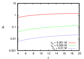
Figure 4: Variation of the cholesteric pitch $qL$ with concentration $c$ for right-handed Yukawa helices with $k=1.4$ and $L/D=50$. The charge density is $\sigma_{c}D=1$ and the reduced Bjerrum length $\lambda_{B}/D=0.1$.

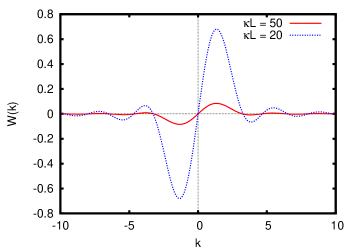
Figure 5: Spatially integrated chiral potential ${\mathcal{W}}(k)$ [Eq. (31)] versus coil pitch $k=2\pi L/p_{\text{int}}$ for identical Yukawa helices with a right-handed ($k>0$) or left-handed ($k<0$) symmetry for $L/D=50$. For ${\mathcal{W}}>0$ a right-handed cholesteric phase is formed, whereas ${\mathcal{W}}<0$ corresponds to a left-handed one. Zero-points indicate a sense inversion of the cholesteric helix at $k=3.25,4.67,6.51,8.00,..$.

III.2 Binary mixtures of helical rods with equal lengths ($\ell=1$)

For a mixture of rods with equal length but different coil pitches ($k_{1}\neq k_{2}$) and/or surfaces charges ($Z_{1}\neq Z_{2}$), the situation is comparable to the monodisperse case since the twist elastic constant is independent of these properties. Furthermore, we have $\alpha_{1}=\alpha_{2}=\alpha$ and the cholesteric pitch is given by a form analogous to Eq. (38):

$$qL\sim\frac{12c}{7}{\bar{\mathcal{E}}}_{c}$$ (40)

in terms of an effective chiral strength given by a simple mole fraction average of the different pair contributions:

$${\bar{\mathcal{E}}}_{c}=\sum_{i}\sum_{j}x_{i}x_{j}{\mathcal{E}}_{c}^{ij}$$ (41)

with ${\mathcal{E}}_{c}^{ij}$ the generalized version of Eq. (39):

$${\mathcal{E}}_{c}^{ij}\sim\left(\frac{\lambda_{B}}{D}\right)^{2}Z_{i}^{2}Z_{j}^{2}\left(\frac{D}{L_{1}}\right)^{3}{\mathcal{W}}(k_{i},k_{j})$$ (42)

III.3 Binary mixtures of helical rods with unequal lengths ($\ell\neq 1$)

In case of a binary mixture of rods with different lengths things are more complicated and most thermodynamic properties such as the cholesteric pitch can only be assessed numerically. Let us first investigate the effect of a weak chiral potential on the phase behavior of rod mixtures with different length ratios. To that end we must first consider the free energy of a binary mixture of infinitely thin hard rods with length ratio $\ell$ in the nematic phase. Within the Gaussian approximation it is given by Odijk and Lekkerkerker (1985); Vroege and Lekkerkerker (1993):

$$\frac{\beta F_{\text{nem}}}{N} \sim \ln c+\sum_{i}x_{i}[\ln x_{i}\alpha_{i}-1]$$ (43)

$$+c\sum_{i}\sum_{j}x_{i}x_{j}\frac{L_{i}L_{j}}{L_{1}^{2}}\left\langle\left\langle\gamma\right\rangle\right\rangle$$

$$\sim \ln c+\sum_{i}x_{i}[\ln x_{i}\alpha_{i}-1]+c\left(\frac{\pi}{\alpha_{1}}\right)^{1/2}$$

$$\times\left[x_{1}^{2}+2^{1/2}x_{1}x_{2}\ell(1+Q^{-1})^{1/2}+x_{2}^{2}\ell^{2}Q^{-1/2}\right]$$

In the isotropic phase the free energy simplifies to:

$$\frac{\beta F_{\text{iso}}}{N}\sim\ln c+\sum_{i}x_{i}\ln x_{i}+c\frac{\pi}{4}\left[x_{1}^{2}+2x_{1}x_{2}\ell+x_{2}^{2}\ell^{2}\right]\\$$ (44)

In the cholesteric phase we must take into account the change of free energy associated with the weak helical distortion of director-field as discussed in the preceding Section:

$$\frac{\beta F_{\text{chol}}}{N}\sim\frac{\beta F_{\text{nem}}}{N}+\frac{1}{c}\sum_{i}\sum_{j}x_{i}x_{j}\left[-\tilde{K}_{1}^{ij}\tilde{q}+\frac{1}{2}\tilde{K}_{2}^{ij}\tilde{q}^{2}\right]$$ (45)

which yields upon minimization with respect to the cholesteric pitch $\tilde{q}=2\pi L_{1}/p$:

$$\frac{\beta F_{\text{chol}}}{N}\sim\frac{\beta F_{\text{nem}}}{N}-\frac{1}{2c}\frac{\left(\sum_{i}\sum_{j}x_{i}x_{j}\tilde{K}_{1}^{ij}\right)^{2}}{\sum_{i}\sum_{j}x_{i}x_{j}\tilde{K}_{2}^{ij}}$$ (46)

We reiterate that this expression is only applicable in the regime $\tilde{q}\ll 1$ where the helical distortion of the director field does not interfere with the local orientational order. Since the twist elastic constants are positive, the second term in the free energy must be negative which implies that a small degree of chirality always leads to a reduction of the free energy of the system. In explicit form, the twist elastic constants for the pure components are given by:

$$\tilde{K}_{2}^{11} = \beta K_{2}^{11}D\sim\frac{7c^{2}}{192}\left(\frac{\pi}{\alpha_{1}}\right)^{1/2}$$

$$\tilde{K}_{2}^{22} = \beta K_{2}^{22}D\sim\frac{7c^{2}}{192}\left(\frac{\pi}{\alpha_{1}}\right)^{1/2}\ell^{4}Q^{-1/2}$$

$$\tilde{K}_{2}^{12} = \beta K_{2}^{12}D\sim\frac{7c^{2}}{192}\left(\frac{\pi}{\alpha_{1}}\right)^{1/2}g(Q)$$ (47)

with

$$g(Q)=2^{1/2}\frac{(3Q^{2}+4Q)\ell+(3+4Q)\ell^{3}}{7Q^{1/2}(1+Q)^{3/2}}$$ (48)

Similarly, one can produce for the torque-field contributions:

$$\tilde{K}_{1}^{ij}=\beta K_{1}^{ij}DL_{1}\sim\frac{c^{2}}{8}{\mathcal{E}}_{c}^{ij}\\$$

With this, the cholesteric free energy of a binary mixture with $\ell\neq 1$ can be rewritten as:

$$\frac{\beta F_{\text{chol}}}{N}\sim\frac{\beta F_{\text{nem}}}{N}-\frac{3c^{2}}{28}G(x_{i},Q){\bar{\mathcal{E}}}_{c}^{2}$$ (49)

with:

$$G(x_{i},Q)=\left(\frac{x_{1}+2^{1/2}x_{2}\ell(1+Q^{-1})^{-1/2}}{x_{1}^{2}+2x_{1}x_{2}g(Q)+x_{2}^{2}\ell^{4}Q^{-1/2}}\right)$$ (50)

The corresponding cholesteric pitch takes the following form:

$$\tilde{q}=\frac{2\pi L_{1}}{p}\sim\frac{12c}{7}{\bar{\mathcal{E}}}_{c}G(x_{i},Q)$$ (51)

As required, this expression reduces to the forms proposed in the previous subsections [Eq. (38) and Eq. (40)] if we substitute $\ell=1$ and $Q=1$. Recalling that $Q=Q(x)$ we conclude that the concentration dependence of the cholesteric pitch of the mixture is identical to that of the monodisperse system. The behavior of the pitch with respect to the mole fraction $x_{2}=1-x_{1}$ on the other hand is expected to be quite rich and this will be scrutinized in detail further on.

Let us now consider a binary mixtures of helical rods with equal charge density $\sigma_{c}$ so that the mole-fraction averaged chiral parameter ${\bar{\mathcal{E}}}_{c}$ can be written in compact form as:

$${\bar{\mathcal{E}}}_{c}=\varepsilon_{0}\left(x_{1}^{2}\varepsilon_{11}+2x_{1}x_{2}\ell^{2}\varepsilon_{12}+x_{2}^{2}\ell^{4}\varepsilon_{22}\right)$$ (52)

in terms of an amplitude $\varepsilon_{0}$ and phase factor $\varepsilon_{ij}$:

$$\varepsilon_{0} = \left(\frac{\lambda_{B}}{D}\right)^{2}\left(\frac{L_{1}}{D}\right)(\sigma_{c}D)^{4}$$

$$\varepsilon_{ij} = {\mathcal{W}}(k_{i},k_{j})$$ (53)

which needs to be specified for the mixture of interest.

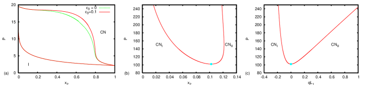
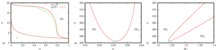
Figure 6: (a) Isotropic-cholesteric nematic phase diagram for a mixture of Yukawa helices with length ratio $\ell=3$ consisting of helices with opposite handedness ($k_{1}=-k_{2}=1.4$). Plotted is the osmotic pressure $P=\beta\Pi L_{1}^{2}D$ versus the mole fraction of the left-handed species $x=x_{2}$. (b) High pressure region featuring a demixing of the cholesteric phase. A critical point is indicated by the dot. (c) Cholesteric pitch of coexisting left- and right-handed cholesteric phases versus pressure. (d)-(f) Same results for a mixture of helices with equal handedness ($k_{1}=k_{2}=1.4$) and $\ell=3$.

Let us first consider the case $\ell=3$ with $k_{1}=-k_{2}=1.4$, i.e. a mixture of short right-handed helices mixed with long left-handed ones with equal pitch magnitude. To simplify matters we shall consider dispersions with excess added salt such that the screening constant is fixed to $\kappa L_{1}=50$, independent of the rod concentration. The phase diagrams of the chiral systems and the corresponding hard rod reference system are shown in Fig. 6. Althought the isotropic-nematic transition is only marginally affected by chirality, the cholesteric phase show a demixing into two coexisting cholesteric fractions with opposite handedness. The demixing region is closed off by a lower critical point located at $qL=0$ indicating that the cholesteric pitch vanishes at the critical point. Note that the achiral mixture do not show this demixing at this particular length ratio. Within the Gaussian approximation Vroege and Lekkerkerker (1993) such a demixing only occurs above a critical length ratio $\ell>3.167$. Moreover, the nematic-nematic binodals do not meet in a lower critical point but merge with the isotropic-nematic ones to produce an isotropic-nematic-nematic triphasic equilibrium, irrespective of the length ratio $\ell$. The cholesteric-cholesteric demixing is driven primarily by the small chiral dispersion contribution to the rod interaction potential and does not arise from an interplay of the various entropic contributions (associated with mixing, free-volume and orientational order) such as for hard rod mixtures. A similar demixing is observed for a mixtures of right-handed helices with $k_{1}=k_{2}=1.4$ at $\ell=3$ and amplitude $\varepsilon_{0}=0.1$, albeit at a much higher osmotic pressure. It is worth noting that for this case the cholesteric pitch does not reduce to zero at the critical point but attains a finite positive value. For the case $\ell=1$, i.e. helices with equal lengths, no demixing of the cholesteric state was found. This shows that a cholesteric mixture of left- and righthanded helices can only demix if the length ratio between the species is considerable.

Fig. 7 shows the behavior of the cholesteric pitch across the range of mole fractions. For the first mixture, a quasi-linear reduction of the pitch is observed accompanied by a change of handedness upon increasing the mole fraction of the left-handed ‘dopant’ helices. The zero-point corresponding to a vanishing pitch is virtually (but not strictly) independent of the osmotic pressure of the suspension. For the second mixture the trend is completely different and features a non-monotonic increase of the pitch with mole fraction. A similar non-monotonic trend is observed for the pitch of a cholesteric phase in coexistence with an isotropic phase as a function of pressure.

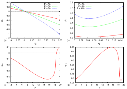
Figure 7: Variation of the cholesteric pitch versus mole fraction at constant pressure. (a) Helices with opposite handedness ($k_{1}=-k_{2}=1.4$, $\ell=3$). (b) Helices with equal handedness ($k_{1}=k_{2}=1.4$, $\ell=3$). (c) Behavior of the pitch as a function of the isotropic-cholesteric coexistence pressure for $k_{1}=-k_{2}=1.4$ and $\ell=3$. (d) Same for $k_{1}=k_{2}=1.4$, $\ell=3$.

IV Discussion and conclusions

It is instructive to compare the present Yukawa-type chiral potential with a much simpler model potential employed in a previous study Ref. Wensink and Jackson, 2009. There, we have used a square well (SW) chiral potential based on the Goossens form Eq. (22):

$$U_{\text{SW}}(\Delta{\bf r};{\bf\hat{u}}_{1},{\bf\hat{u}}_{2})=-\varepsilon_{\text{SW}}H(\Delta r-\lambda)({\bf\hat{u}}_{1}\cdot{\bf\hat{u}}_{2})\chi$$ (54)

with $H(\Delta r-\lambda)$ a Heaviside step function. The main parameters characterizing the chiral interaction are the SW range $\lambda>(1+D/L)$ and depth $\varepsilon_{\text{SW}}$. The main advantage of using the SW form is it that it renders the spatial integrations over the potential analytically tractable. The result for the torque field constant is very simple: $\beta K_{1}D^{2}\sim(\pi c^{2}/6)\beta\varepsilon_{\text{SW}}\lambda^{4}$. Comparing this with Eq. (34) and setting the reduced SW range $\lambda$ to unity allows us to make an explicit link between the SW depth and the microscopic parameters pertaining to the electrostatic interactions between the helices:

$$\beta\varepsilon_{\text{SW}}\sim\frac{3Z^{4}}{4\pi}\left(\frac{\lambda_{B}}{D}\right)^{2}\left(\frac{D}{L}\right)^{4}{\mathcal{W}}(k)$$ (55)

The justification for this relation lies in the notion that most thermodynamic properties are governed by the spatially integrated pair potential rather than the bare one. A prominent example is the classical van der Waals model for fluids whose universal nature stems from the fact that any arbitrary (but weakly) attractive potential can be mapped onto a single integrated van der Waals energy which, along with the excluded-volume contribution, fully determines the equation of state and hence the thermodynamics of the fluid state.

In summary, we have proposed a helical Yukawa segment model as a course-grained model in an effort to quantify the chiral interaction between stiff chiral polyelectrolytes. Our chiral potential strongly resembles the classic Goossens potential Goossens (1971), which has been used almost exclusively to describe long-ranged chiral dispersion forces. Contrary to the Goossens form, our potential provides an explicit reference to the microscopic and electrostatic properties of the rods. Combining the potential with a simple second-virial theory allows us to study the structure and thermodynamic stability of the cholesteric state as a function of rod density, degree of coiling, and electrostatic screening. While the magnitude of the cholesteric pitch depends strongly on the rod concentration and concentration of added salt, the handedness of the phase is governed mainly by the pitch of the Yukawa coil. The symmetry of the cholesteric phase need not be equivalent to that of the individual helices but may be different, depending on the precise value of the coil pitch. Within a certain interval of the coil pitch, right-handed Yukawa coils may generate left-handed cholesteric order and vice versa. The antagonistic effect of charge-mediated chiral interactions is consistent with experimental observations in M13 virus systems Tombolato et al. (2006) and various types of DNA Livolant and Leforestier (1996); Tombolato and Ferrarini (2005) where left-handed cholesteric phases are formed from right-handed helical polyelectrolyte conformations. Small variations in the shape of the helical coil, induced by e.g. a change of temperature, may lead to a sense inversion of the cholesteric helix. Such an inversion has been found in thermotropic (solvent free) polypeptides Watanabe and Nagase (1988) and cellulose derivatives Yamagishi et al. (1990), and in mixtures of right-handed cholesterol chloride and left-handed cholesterol myristate Sackmann et al. (1968).

Our model also predicts that a very small degree of microscopic helicity is required to maximize the twisting potential of the Yukawa helices. The optimum is reached when the pitch distance of the coils equals about $5$ times the rod length. Mixing stiff helical rods with sufficiently different lengths may lead to a demixing of the cholesteric phase at high pressures. The demixing region closes off at a critical point upon lowering the osmotic pressure.

The present model could be interpreted as a simple prototype for complex biomacromolecules such as DNA and fd which are characterized by a helical distribution of charged surface groups. Other lyotropic cholesteric systems, such as cellulose and chitin microfibers in solution could also be conceived as charged rods with a twisted charge distribution Revol and Marchessault (1993). Small changes in the internal twist of the fibrils could be induced (e.g. by applying an external field or varying the temperature) in order to tune the handedness of the cholesteric phase. This could be of importance for the use of chiral nanocrystals in optical switching devices and nanocomposites. We remark that a more accurate description of the pitch sensitivity, particularly for DNA systems, could be formulated by accounting for the steric contributions associated with the helical backbone of the chains as well as the influence of chain flexibility. This could open up a route towards understanding the unusual behaviour of the pitch versus particle and salt concentration as encountered in DNA Livolant and Leforestier (1996); Stanley et al. (2005) using simple coarse-grained models. Furthermore, a quantitative comparison of the predicted pitch distances with experimental systems should be possible for rigid, slender polyelectrolytes with a well-defined surface charge and internal pitch. Most chiral systems studied to date however do not fulfill these criteria which makes it difficult to put our predictions to a quantitative test. At present, our theory should therefore be considered as a mere qualitative guideline.

Future work will be aimed at studying the pitch sensitivity beyond the purely Gaussian approximation. This can be done by adopting a numerical approach to determine the local ODF in a self-consistent way. This approach could unveil a much more complex relation between the pitch handedness and system density (or temperature) as suggested by the intricate angle-dependence of the chiral potential in Fig. 2. Such a sense inversion upon changing temperature has been found theoretically by Kimura et al.Kimura et al. (1979, 1982) within a simple mean-field (Maier-Saupe) treatment of the hard rod model combined with a Goossens-type chiral potential. It would be intriguing to see whether a similar effect could be generated from the present Yukawa model. Investigations along these lines are currently being undertaken.

Appendix: Gaussian averages

The Gaussian averages required for the calculation of the twist elastic constant are taken from Ref. Odijk, 1986. We quote them here:

$$\left\langle\left\langle\gamma\right\rangle\right\rangle \sim \left(\frac{\pi}{2}\right)^{1/2}\left(\frac{\alpha_{i}+\alpha_{j}}{\alpha_{i}\alpha_{j}}\right)^{1/2}$$ (56)

$$\left\langle\left\langle\gamma^{3}\theta_{i}^{2}\right\rangle\right\rangle \sim 3\left(\frac{\pi}{2}\right)^{1/2}\left(\frac{\alpha_{i}+\alpha_{j}}{\alpha_{i}\alpha_{j}}\right)^{1/2}\left(\frac{2\alpha_{i}+5\alpha_{j}}{\alpha_{i}^{2}\alpha_{j}}\right)$$ (57)

$$\left\langle\left\langle\gamma\theta_{i}^{2}(\theta_{i}^{2}+\theta_{j}^{2})\right\rangle\right\rangle \sim \left(\frac{\pi}{2}\right)^{1/2}\left(\frac{6\alpha_{i}^{3}+19\alpha_{i}^{2}\alpha_{j}+30\alpha_{i}\alpha_{j}^{2}+15\alpha_{j}^{3}}{\alpha_{i}^{5/2}\alpha_{j}^{3/2}(\alpha_{i}+\alpha_{j})^{3/2}}\right)$$ (58)

References

- de Gennes and Prost (1993) P. G. de Gennes and J. Prost, The Physics of Liquid Crystals (Clarendon Press, Oxford, 1993).
- Aharoni (1979) S. M. Aharoni, Macromolecules 12, 94 (1979).
- Sato et al. (1993) T. Sato, Y. Sato, Y. Umemura, A. Teramoto, Y. Nagamura, J. Wagner, D. Weng, Y. Okamoto, K. Hatada, and M. M. Green, Macromolecules 26, 4551 (1993).
- Watanabe et al. (2001) J. Watanabe, H. Kamee, and M. Fujiki, Polym. J. 33, 495 (2001).
- Robinson (1961) C. Robinson, Tetrahedron 13, 219 (1961).
- Livolant and Leforestier (1996) F. Livolant and A. Leforestier, Prog. Polym. Sci. 21, 1115 (1996).
- Dogic and Fraden (2006) Z. Dogic and S. Fraden, Curr. Opin. Colloid Interface Sci. 11, 47 (2006).
- Uematsu and Uematsu (1984) I. Uematsu and Y. Uematsu, Adv. Pol. Sci. 59, 37 (1984).
- DuPré and Samulski (1979) D. B. DuPré and E. T. Samulski, in Liquid Crystals: the Fourth State of Matter, edited by F. D. Saeva (Dekker, New York, 1979).
- Hiltrop (2001) K. Hiltrop, in Chirality in Liquid Crystals, edited by H. S. Kitzerow and C. Bahr (Springer-Verlag, New York, 2001).
- Sato and Teramoto (1996) T. Sato and A. Teramoto, Adv. Polym. Sci. 126, 85 (1996).
- Werbowyj and Gray (1976) R. S. Werbowyj and D. G. Gray, Mol. Cryst. Liquid Cryst. 34, 97 (1976).
- Revol and Marchessault (1993) J.-F. Revol and R. H. Marchessault, Int. J. Biol. Macromol. 15, 329 (1993).
- van Winkle et al. (1990) D. H. van Winkle, M. W. Davidson, W. X. Chen, and R. L. Rill, Macromolecules 23, 4140 (1990).
- Yevdokimov et al. (1988) Y. M. Yevdokimov, S. G. Skuridin, and V. I. Salyanov, Liq. Cryst. 3, 1443 (1988).
- Stanley et al. (2005) C. B. Stanley, H. Hong, and H. H. Strey, Biophys. J. 89, 2552 (2005).
- Dogic and Fraden (2000) Z. Dogic and S. Fraden, Langmuir 16, 7820 (2000).
- Grelet and Fraden (2003) E. Grelet and S. Fraden, Phys. Rev. Lett. 90, 198302 (2003).
- DuPré and Duke (1975) D. B. DuPré and R. W. Duke, J. Chem. Phys. 63, 143 (1975).
- Yoshiba et al. (2003) K. Yoshiba, A. Teramoto, N. Nakamura, and T. Sato, Macromolecules 36, 2108 (2003).
- Dong and Gray (1997) X. M. Dong and D. G. Gray, Langmuir 13, 2404 (1997).
- Miller and Donald (2003) A. F. Miller and A. M. Donald, Biomacromolecules 4, 510 (2003).
- Dong et al. (1996) X. M. Dong, T. Kimura, J. F. Revol, and D. G. Gray, Langmuir 12, 2076 (1996).
- Straley (1973) J. P. Straley, Phys. Rev. A 8, 2181 (1973).
- Jákli et al. (2007) A. Jákli, C. Bailey, and J. Harden, in Thermotropic Liquid Crystals, edited by A. Ramamoorthi (Springer, Netherlands, 2007), p. 59.
- Odijk (1987) T. Odijk, J. Phys. Chem. 91, 6060 (1987).
- Kimura et al. (1982) H. Kimura, M. Hosino, and H. Nakano, J. Phys. Soc. Jpn. 51, 1584 (1982).
- Orts et al. (1998) W. J. Orts, L. Godbout, R. H. Marchessault, and J.-F. Revol, Macromolecules 31, 5717 (1998).
- Pelcovits (1996) R. A. Pelcovits, Liq. Cryst. 21, 361 (1996).
- Harris et al. (1999) A. B. Harris, R. D. Kamien, and T. C. Lubensky, Rev. Mod. Phys. 71, 1745 (1999).
- Strey et al. (1998) H. H. Strey, R. Podgornik, D. C. Rau, and V. A. Parsegian, Curr. Opin. Struct. Biol. 3, 534 (1998).
- Kornyshev and Leikin (1997) A. A. Kornyshev and S. Leikin, J. Chem. Phys. 107, 3656 (1997).
- Kornyshev and Leikin (2000) A. A. Kornyshev and S. Leikin, Phys. Rev. Lett. 84, 2537 (2000).
- Kornyshev et al. (2002) A. A. Kornyshev, S. Leikin, and S. V. Malinin, Eur. Phys. J. E 7, 83 (2002).
- Tombolato and Ferrarini (2005) F. Tombolato and A. Ferrarini, J. Chem. Phys. 122, 054908 (2005).
- Goossens (1971) W. J. A. Goossens, Mol. Cryst. Liq. Cryst. 12, 237 (1971).
- van der Meer and Vertogen (1979) B. W. van der Meer and G. Vertogen, in The Molecular Physics of Liquid Crystals, edited by G. R. Luckhurst and G. W. Gray (Academic Press, New York, 1979).
- van der Meer et al. (1976) B. W. van der Meer, G. Vertogen, A. J. Dekker, and J. G. J. Ypma, J. Chem. Phys. 65, 3935 (1976).
- Lin-Liu et al. (1977) Y. R. Lin-Liu, Y. M. Shih, and C. W. Woo, Phys. Rev. A 15, 2550 (1977).
- Hu et al. (1998) L. Hu, Y. Jiang, T. D. Lee, and R. Tao, Phys. Rev. E 57, 4289 (1998).
- Osipov and Kuball (2001) M. A. Osipov and H.-G. Kuball, Eur. Phys. J. E 5, 589 (2001).
- Kapanowski (2002) A. Kapanowski, Z. Naturforsch. 57A, 105 (2002).
- Emelyanenko (2003) A. V. Emelyanenko, Phys. Rev. E 67, 031704 (2003).
- Onsager (1949) L. Onsager, Ann. N.Y. Acad. Sci. 51, 627 (1949).
- Varga and Jackson (2006) S. Varga and G. Jackson, Mol. Phys. 104, 3681 (2006).
- Wensink and Jackson (2009) H. H. Wensink and G. Jackson, J. Chem. Phys. 130, 234911 (2009).
- Yi et al. (2008) J. Yi, Q. Xu, X. Zhang, and H. Zhang, Polymer 49, 4406 (2008).
- Barry et al. (2009) E. Barry, D. Beller, and Z. Dogic, Soft Matter 5, 2563 (2009).
- Tombolato et al. (2006) F. Tombolato, A. Ferrarini, and E. Grelet, Phys. Rev. Lett. 96, 258302 (2006).
- Hansen and McDonald (2006) J. P. Hansen and I. R. McDonald, Theory of Simple Liquids (Academic Press, New York, 2006).
- Kirchhoff et al. (1996) T. Kirchhoff, H. Löwen, and R. Klein, Phys. Rev. E 53, 5011 (1996).
- Israelachvili (1991) J. N. Israelachvili, Intermolecular and surface forces (Academic Press, London, 1991).
- Rushbrooke (1940) G. S. Rushbrooke, Trans. Faraday. Soc. 36, 1055 (1940).
- Rowlinson (1958) J. S. Rowlinson, Mol. Phys. 1, 414 (1958).
- Straley (1976) J. P. Straley, Phys. Rev. A 14, 1835 (1976).
- Allen et al. (1993) M. P. Allen, G. T. Evans, D. Frenkel, and B. M. Mulder, Adv. Chem. Phys. 86, 1 (1993).
- Gelbart and Baron (1977) W. M. Gelbart and B. A. Baron, J. Chem. Phys. 66, 207 (1977).
- Franco-Melgar et al. (2008) M. Franco-Melgar, A. J. Haslam, and G. Jackson, Mol. Phys. 106, 649 (2008).
- Odijk and Lekkerkerker (1985) T. Odijk and H. N. W. Lekkerkerker, J. Phys. Chem. 89, 2090 (1985).
- Vroege and Lekkerkerker (1993) G. J. Vroege and H. N. W. Lekkerkerker, J. Phys. Chem. 97, 3601 (1993).
- Watanabe and Nagase (1988) J. Watanabe and T. Nagase, Macromolecules 21, 171 (1988).
- Yamagishi et al. (1990) T. Yamagishi, T. Fukada, T. Miyamoto, T. Ichizuka, and J. Watanabe, Liq. Cryst. 7, 155 (1990).
- Sackmann et al. (1968) E. Sackmann, S. Meiboom, L. C. Snyder, A. E. Meixner, and R. E. Dietz, J. Am. Chem. Soc. 90, 3567 (1968).
- Kimura et al. (1979) H. Kimura, M. Hosino, and H. Nakano, J. Phys. Colloques 40, 174 (1979).
- Odijk (1986) T. Odijk, Liq. Cryst. 1, 553 (1986).