Analysis of optical Fe II emission in a sample of AGN spectra

Abstract

We present a study of optical Fe II emission in 302 AGNs selected from the SDSS. We group the strongest Fe II multiplets into three groups according to the lower term of the transition (b${\ }^{4}F$, a${\ }^{6}S$ and a${\ }^{4}G$ terms). These correspond approximately to the blue, central, and red part respectively of the “iron shelf” around H$\beta$. We calculate an Fe II template which takes into account transitions into these three terms and an additional group of lines, based on a reconstruction of the spectrum of I Zw 1. This Fe II template gives a more precise fit of the Fe II lines in broad-line AGNs than other templates. We extract Fe II, H$\alpha$, H$\beta$, [O III] and [N II] emission parameters and investigate correlations between them. We find that Fe II lines probably originate in an Intermediate Line Region. We notice that the blue, red, and central parts of the iron shelf have different relative intensities in different objects. Their ratios depend on continuum luminosity, FWHM H$\beta$, the velocity shift of Fe II, and the $\mathrm{H\alpha}$/$\mathrm{H\beta}$ flux ratio. We examine the dependence of the well-known anti-correlation between the equivalent widths of Fe II and [O III] on continuum luminosity. We find that there is a Baldwin effect for [O III] but an inverse Baldwin effect for the Fe II emission. The [O III]/Fe II ratio thus decreases with L_λ5100. Since the ratio is a major component of the Boroson and Green eigenvector 1, this implies a connection between the Baldwin effect and eigenvector 1, and could be connected with AGN evolution. We find that spectra are different for H$\beta$ FWHMs greater and less than $\sim$3000 $\mathrm{kms^{-1}}$, and that there are different correlation coefficients between the parameters.

1 Introduction

Optical Fe II ($\lambda\lambda$ 4400-5400 Å) emission is one of the most interesting features in AGN spectra. The emission arises from numerous transitions of the complex Fe II ion. Fe II emission is seen in almost all type-1 AGN spectra and it is especially strong in narrow-line Seyfert 1s (NLS1s). It can also appear in the polarized flux of type-2 AGNs when a hidden BLR can be seen. Origin of the optical Fe II lines, the mechanisms of their excitation and location of the Fe II emission region in AGN, are still open questions. There are also many correlations between Fe II emission and other AGN properties which need a physical explanation.

Some of the problems connected with Fe II emission are:

1. There have been suggestions that Fe II emission cannot be explained with standard photoionization models (see Collin & Joly, 2000; Collin-Souffrin et al., 1980, and references therein). To explain the Fe II emission, additional mechanisms of excitation have been proposed: a) continuum fluorescence (Phillips, 1978a, 1979), b) collisional excitation (Joly, 1981, 1987, 1991; Veron et al., 2006), c) self-fluorescence among Fe II transitions (Netzer & Wills, 1983), d) fluorescent excitation by the Ly$\alpha$ and Ly$\beta$ lines (Penston, 1988; Verner et al., 1999).

2. There are uncertainties about where the Fe II emission line region is located in an AGN. A few proposed solutions are that the Fe II lines arise: a) in the same emission region as the broad H$\beta$ line (Boroson & Green, 1992), b) in the accretion disk near the central black hole, which produces the double-peaked broad Balmer emission lines (Collin-Souffrin et al., 1980; Zhang et al., 2006), c) in a region which can be heated by shocks or from an inflow, located between BLR and NLR – the so-called the Intermediate Line Region (Marziani & Sulentic, 1993; Popović et al., 2004, 2007, 2009; Hu et al., 2008a; Kuehn et al., 2008) and d) and in the shielded, neutral, outer region of a flattened BLR (Gaskell et al., 2007; Gaskell, 2009).

3. It has long been established that the Fe II emission is correlated with the radio, X and IR continuum. Fe II lines are stronger in spectra of Radio Quiet (RQ) AGNs, than in Radio Loud (RL) objects (Osterbrock, 1977; Bergeron & Kunth, 1984). But, if we consider RL AGNs, Fe II emission is stronger in Core Dominant (CD) AGNs than in Lobe Dominant (LD) AGNs (Setti & Woltjer, 1977; Joly, 1991). The relative strength of the Fe II lines correlates with the soft X-ray slope, but anti-correlates with X-ray luminosity (Wilkes et al., 1987; Boller et al., 1996; Lawrence et al., 1997). Strong optical Fe II emission is usually associated with strong IR luminosity (Low et al., 1989; Lipari et al., 1993), but it is anti-correlated with IR color index $\alpha$(60,25) (Wang et al., 2006).

4. Many correlations have been observed between Fe II and other emission lines. Boroson & Green (1992) give a number of correlations between the equivalent width (EW) of Fe II and properties of the [O III] and H$\beta$ lines. The most interesting are the anti-correlations of EW Fe II vs. EW [O III]/EW H$\beta$, EW Fe II vs. peak [O III], EW Fe II/EW H$\beta$ vs. peak [O III], and the correlation of EW Fe II/EW H$\beta$ vs. H$\beta$ asymmetry. An anti-correlation between EW Fe II and FWHM of H$\beta$ has been also found (Gaskell, 1985; Zheng & Keel, 1991; Boroson & Green, 1992). These correlations dominate the first eigenvector of the principal component analysis of Boroson & Green (1992) (hereinafter EV1). Correlations between EV1 and some properties of C IV $\lambda 1549$ Å lines have also been pointed out (Baskin & Laor, 2004). With increasing continuum luminosity, the EW of the C IV lines decreases, (the so-called “Baldwin effect”, Baldwin, 1977; Wang et al., 1995), while the blueshift of the C IV line and the EW of Fe II increase. Recently, Dong et al. (2009) have found the Baldwin effect to be related to EV1. Fe II lines are usually strong in AGN spectra with low-ionization Broad Absorption Lines (BALs) (Harting & Baldwin, 1986; Boroson & Meyers, 1992).

Searching for a physical cause of these correlations may help in understanding of the origin of Fe II emission. Some of physical properties which may influence these correlations are: Eddington ratio (L/$\mathrm{L_{Edd}}$) (Boroson & Green, 1992; Baskin & Laor, 2004), black hole mass ($M_{BH}$) and inclination angle (Miley & Miller, 1979; Wills & Browne, 1986; Marziani et al., 2001).

In addition to these properties, Fe II emission strength may vary with evolution of AGNs. For example, Lipari & Terlevich (2006) have explained some properties of AGN (as BALs, Fe II strength, radio properties, emission line width, luminosity of narrow lines, etc.) by an “evolutive unification model”. In this model, accretion arises from the interaction between nuclear starbursts and the supermassive black hole. This would mean that not only the orientation, but also the evolutionary state of an AGN, influence its spectral properties. Thus, young AGN have strong Fe II, BALs, weak radio emission, the NLR is compact and faint, and broad lines are relatively narrow. In contrast with this, old AGNs have weak Fe II, no BALs, strong radio emission with extended radio lobes, the NLR is extended and bright, and the broad lines have greater velocity widths.

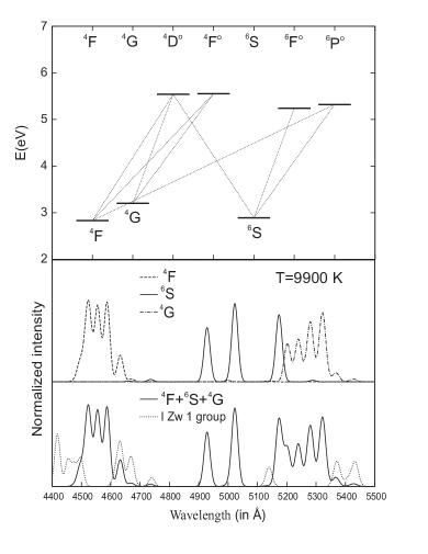
Figure 1: Grotrian diagram showing the strongest Fe II transitions in the $\lambda\lambda$ 4400-5500 Å region (top). Lines are separated into three groups according to the lower level of transition (middle): $F$ (dashed line), $S$ (solid line) and $G$ (dash–dotted line). Bottom: the lines from the three line groups (solid line) and lines measured from I Zw 1, represented with dots.

In this paper, we investigate the Fe II emitting region by analyzing the correlations between the optical Fe II lines and the other emission lines in a sample of 302 AGN from the SDSS. To do this we construct an Fe II template. The strongest Fe II multiplets within the $\lambda\lambda$4400-5500 Å range are sorted into three groups, according to the lower terms of the transitions: $3d^{6}({\ }^{3}F2)4s{\ }^{4}F$, $3d^{5}4s^{2}{\ }^{6}S$ and $3d^{6}({\ }^{3}G)4s{\ }^{4}G$ (which we will hereinafter refer to as the $F$, $S$ and $G$ groups of lines). The $F$ group mainly contains the lines from the Fe II multiplets 37 and 38 and describes the blue part of the Fe II shelf relative to H$\beta$. The $S$ group of lines describes the part of Fe II emission under H$\beta$ and [O III] and contains lines from multiples 41, 42 and 43 Fe II. Finally, the $G$ group contains lines from multiplets 48 and 49, and describes the red part of the Fe II shelf. A simplified Grotrian diagram of these transitions is shown in Figure 1. We analyze separately their relationships with other lines in AGN spectra (H$\beta$, [O III], H$\alpha$, [N II]). In this way, we try to connect details of the Fe II emission with physical properties of the AGN emission regions in which these lines arise. Each of the Fe II multiplet groups has specific characteristics, which may be reflected in a different percent of correlations with other lines, and give us more information about the complex Fe II emission region.

The paper is organized as follows: In Sect. 2 we describe the procedure of sample selection and details of analysis; our results are presented in Sect. 3; in Sect. 4 we give discussion of obtained results, and finally in Sect. 5 we outline our conclusions.

2 The sample and analysis

2.1 The AGN sample

Spectra for our data sample are taken from the the $7^{th}$ data release (Abazajian et al., 2009) of the Sloan Digital Sky Survey (SDSS). For the purposes of the work, we chose AGNs with the following characteristics:

1. high signal to noise ratio ($\mathrm{S/N}>20$),

2. good pixel quality (profiles are not affected by distortions due to bad pixels on the sensors, the presence of strong foreground or background sources),

3. high redshift confidence (zConf$>$0.95) and with $z\leq 0.7$ in order to cover the optical Fe II lines around H$\beta$ and [O III] lines,

4. negligible contribution from the stellar component. We controlled for this by having the EWs of typical absorption lines be less then 1 Å (EW CaK 3934 Å, Mg 5177 Å and H$\delta$ 4102 Å$>$-1). Because of this it was not necessary to remove a host galaxy starlight contribution.

5. presence of the narrow [O III] and the broad H$\beta$ component (FWHM $\mathrm{H\beta>1000\ kms^{-1}}$).

We found 497 AGNs using the mentioned criteria. However, on inspection of the spectra we found that in some of them the Fe II line emission is within the level of noise and could not be properly fitted, so we excluded these objects from further analysis (see Appendix A). As result, our final sample contains 302 spectra, from which 137 have all Balmer lines, and the rest are without the H$\alpha$ line (due to cosmological redshifts). The sample distribution by continuum luminosity ($\lambda$ 5100 Å) and by cosmological redshift is given in Figure 2. Corrections for Galactic extinction were made using an empirical selective extinction function computed for each spectrum on the basis of Galactic extinction coefficients given by Schlegel (1998) and available from the NASA/IPAC Extragalactic Database. Finally, all spectra were de-redshifted.

To subtract the continuum, we used the DIPSO software, finding the continuum level by using continuum windows given in the paper of Kuraszkiewicz et al. (2002) (see Figure 3). The used continuum windows are: 3010-3040 Å, 3240-3270 Å, 3790-3810 Å, 4210-4230 Å, 5080-5100 Å, 5600-5630 Å and 5970-6000 Å. We used the same procedure to subtract the continuum in all objects. Continuum subtraction may cause systemic errors in the estimation of line parameters and continuum luminosity. We estimated that the error bars are smaller than 5%, especially within the H$\alpha$+[N II] region and in the red part of the “iron shelf”.

We considered two spectral ranges: $\lambda\lambda$ 4400-5500 Å and $\lambda\lambda$ 6400-6800 Å. In the first range, dominant lines are the numerous Fe II lines, [O III] $\lambda\lambda$4959, 5007 Å, H$\beta$ and He II $\lambda$4686 Å, and in the second range, H$\alpha$ and [N II] $\lambda\lambda$6548, 6583 Å.

To investigate correlations between the Fe II multiplets and other lines in spectra, we fit all considered lines with Gaussians. The optical Fe II lines were fitted with a template calculated as described in the next section.

2.2 The Fe II ($\lambda\lambda$ 4400-5500 Å) template

A number of authors have created an Fe II template in the UV and optical range (see Vestergaard & Wilkes, 2001, and references therein). Boroson & Green (1992) applied empirical template by removing all lines which are not Fe II, from the spectrum of I Zw 1. Similarly, Veron-Cetty et al. (2004) constructed an Fe II template by identifying systems of broad and of narrow Fe II lines in the I Zw 1 spectrum, and measuring their relative intensities. Dong et al. (2008) improve on that template by using two parameters of intensity - one for the broad, one for the narrow Fe II lines. All these empirical templates are defined by the line width and the line strength, implying that relative strengths of the lines in the Fe II multiplets are the same in all objects.

In theoretical modeling, significant effort has been made to calculate the iron emission by including a large number of Fe II atomic levels, going to high energy (Verner et al., 1999; Sigut & Pradhan, 2003; Collin-Souffrin et al., 1980; Bruhweiler & Verner, 2008). Bruhweiler & Verner (2008) calculated Fe II emission using CLOUDY code and 830 level Fe II model. In this model, energies go up to 14.6 eV, producing 344,035 atomic transitions. For their calculations they used solar abundances for a range of physical conditions such as the flux of ionizing photons [$\mathrm{\Phi_{H}}$], hydrogen density [$\mathrm{n_{H}}$], and microturbulence [$\xi$].

Using existing Fe II templates, we found that empirical and theoretical models can generally fit NLSy1 Fe II lines well, but that in some cases of spectra with broader H$\beta$ lines, the existing models did not provide as good fit.

One of the problems in the analysis of Fe II emission is that it consists of numerous overlapping lines. This makes the identification and determination of relative intensities very difficult. Therefore, the list of Fe II lines used for the fit of the Fe II emission, as well as their relative intensities, are different in different models (Veron-Cetty et al., 2004; Bruhweiler & Verner, 2008). Also, there is significant disagreement in values of oscillator strengths in different atomic data sources (Fuhr et al., 1981; Giridhar & Ferro, 1995; Kurucz, 1990).

To investigate the Fe II emission, we made an Fe II template taking into account following: (a) majority of multiplets dominant in the optical part ($\lambda\lambda$ 4400-5500 Å), whose lines can be clearly identified in AGN spectra, have one of the three specific lower terms of their transitions: $F$, $S$ or $G$, and (b) beside these lines there are also lines whose origin is not well known but which presumably originate from higher levels.

We constructed an Fe II template consisting of 50 Fe II emission lines, identified as the strongest within $\lambda\lambda$ 4400-5500 Å range. 35 of them are sorted into three line groups according to the lower term of their transition ($F$, $S$ and $G$). The $F$ group consists of 19 lines (mainly multiplets 37 and 38) and dominates in the blue shelf of the iron template (4400-4700 Å). The $S$ group consists of 5 lines (multiplets 41, 42 and 43) and describes the Fe II emission covering the [O III] and H$\beta$ region of the spectrum and some of emission from the red Fe II bump (5150-5400 Å), and the $G$ lines (11 lines from multiplets 48 and 49) dominate in the red bump (5150-5400 Å) (see Figure 1).

We assume that the profiles of each of lines can be represented by a Gaussian, described by width ($W$), shift ($d$) and intensity ($I$). Since all Fe II lines from the template probably originate in the same region, with the same kinematical properties, values of $d$ and $W$ are assumed to be the same for all Fe II lines in the case of one AGN.

Since the population of the lower term is influenced by transition probabilities and excitation temperature, we assumed that the relative intensities between lines within a line group ($F$, $S$ or $G$) can be obtained approximately from:

$$\frac{I_{1}}{I_{2}}={(\frac{\lambda_{2}}{\lambda_{1}})}^{3}\frac{f_{1}}{f_{2}}\cdot\frac{g_{1}}{g_{2}}\cdot e^{-(E_{1}-E_{2})/kT}$$ (1)

where $I_{1}$ and $I_{2}$ are the intensities of lines with the same lower term, $\lambda_{1}$ and $\lambda_{2}$ are the wavelengths of the transition, $g_{1}$ and $g_{2}$ are the statistical weights for the upper energy levels, $f_{1}$ and $f_{2}$ are the oscillator strengths, $E_{1}$ and $E_{2}$ are the energies of the upper levels of transitions, $k$ is the Boltzman constant, and $T$ is the excitation temperature. Details can be found in Appendix C. The excitation temperature is the same for all transitions in the case of partial LTE (see Griem, 1997), but as it is shown in Appendix C, Eq (1) may be used also in some non-LTE cases.

Lines from the three above mentioned groups explain about 75% of the Fe II emission in the observed range (4400-5500 Å), but about 25% of Fe II emission cannot be explained with permitted lines for which the excitation energies are close to the lines of the three groups. The missing Fe II emission is around $\sim$4450 Å, $\sim$4630 Å, $\sim$5130 Å and $\sim$5370 Å.

There are some indications that fluorescence processes may have a role in producing some Fe II lines (Verner et al., 1999; Hartman & Johansson, 2000). Process like self-fluorescence, continuum-fluorescence or Ly$\alpha$ and Ly$\beta$ pumping could supply enough energy to excite the Fe II lines with high energy of excitation, which could be one of the explanation for emission within these wavelength regions. To complete the template for approximately of 25% missing Fe II flux, we selected 15 lines from the Kurutz database with wavelengths close to those of the extra emission, upper level excitation energies of up to $\sim$13 eV, and strong oscillator strengths. We measured their relative intensities in I Zw 1 which has a well-studied spectrum (Veron-Cetty et al., 2004) spectrum with strong and narrow Fe II lines. Relative intensities of these 15 lines were obtained by making the best fit of the I Zw 1 spectrum with the Fe II lines from the $F$, $S$, and $G$ line groups. The extra lines are represented in Figure 1 (bottom), with a dotted line.

Our template of Fe II is described by 7 free fitting parameters: width, shift, four parameters of intensity (for the $F$, $S$ and $G$ line groups and for the lines with relative intensities obtained from I Zw 1). The seventh parameter is the excitation temperature included in the calculation of relative intensities within $F$, $S$ and $G$ line groups.

We found that for the majority of objects, the excitation temperature obtained from our fit is within the range: 9000 K – 11000 K (see Figure 4), which agrees well with theoretical predictions (Collin & Joly, 2000). However, as it could be seen in Eq. (1), our fit is not very sensitive to the temperature, especially for T$>$8000 K. Eq. (1) is also very approximate so estimated temperatures should be treated with caution.

To estimate the error in the excitation temperature, we found our best fit for a number of objects. We then changed only the excitation temperature while keeping the other fit parameters fixed. We thus found $\chi^{2}_{max}$ for which the fit is still reasonable. After that, we constructed $\chi^{2}$ vs. $T$ and measured the dispersion in temperature at 0.1$\cdot$($\chi^{2}_{max}$-$\chi^{2}_{min}$). We obtained error-bars that were mostly within the range $\pm 25\%$, with tendency for higher temperature to have a greater uncertainty. In further analysis we will therefore not consider the temperatures obtained from the fit.

The wavelengths of the 50 template lines are presented in Tables 1 and 2. For the 35 lines from the three line groups we give multiplet names, configurations of the transitions generating those lines, oscillator strengths and the relative intensities. The intensities have been calculated using the Eq. (1) for excitation temperatures $T$ = 5000, 10000 and 15000 K (Table 1). For the 15 lines for which relative intensities were measured in I Zw 1, we give wavelengths, configurations and oscillator strengths taken from Kurucz database, as well as their measured relative intensities (Table 2).

The purpose of dividing the Fe II emission into four groups is to investigate the correlations between the iron lines which arise from different multiplets and some spectral properties, and to compare it with results obtained for the total Fe II within the observed range. Also, a template which has more parameters may give a better fit, since relative intensities among Fe II lines can be different even in the similar AGN spectra, as is, for example, the case for spectra of I Zw 1 and Mrk 42 (as e.g. Phillips, 1978b).

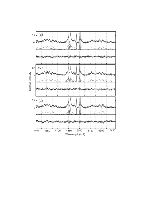
Figure 23: Examples of fits to SDSS J020039.15-084554.9: with our template (a), with the empirical template of Dong et al. (2008) (b), and with the theoretical template of Bruhweiler & Verner (2008) (c). Since this AGN has iron emission equally strong in blue and red iron bump (as I Zw 1), all three models fit the observed lines well.

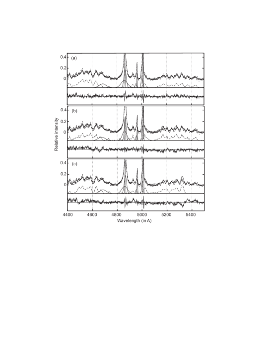
Figure 24: Examples of fits to SDSS J$141755.54+431155.8$: with our template (a), with the empirical template of Dong et al. (2008) (b), and with the theoretical template of Bruhweiler & Verner (2008) (c). Iron emission is a bit stronger in the blue bump, than in red. Our model fits this spectrum slightly better than other two.

We applied this template to our sample of 302 AGNs from SDSS database, and we compare it with other theoretical and empirical models (see Appendix B). We found that the template fit Fe II emission very well (Figure 23 and Figure 24). In the cases when the Fe II emission of an object has different properties from I Zw 1, small disagreements are noticed in the lines for which the relative intensity was obtained from I Zw 1. However, the Fe II emission in these objects shows larger disagreement with the empirical and theoretical models considered in Appendix B (see Figure 25). Although our Fe II template has more free parameters than other templates used for fitting the Fe II emission, it enables more precise fit of Fe II lines in some AGNs (especially with very broad H$\beta$ line) than the other Fe II templates we considered.

2.3 Emission line decomposition and fitting procedure

We assume that broad emission lines arise in two or more emission regions (Brotherton et al., 1994; Popović et al., 2004; Bon et al., 2006, 2009; Ilić et al., 2006), so that their profiles are sums of Gaussians with different shifts, widths and intensities, which reflect the physical conditions of the emitting regions where the components arise.

For this reason, we fit the emission lines we considered ([O III] $\lambda\lambda$4959, 5007 Å, H$\beta$, He II $\lambda$4686 Å, H$\alpha$ and [N II] $\lambda\lambda$6548, 6583 Å) with a sum of Gaussians, describing one Gaussian with 3 parameters (width, intensity and shift from transition wavelength).

Both lines of the [O III] $\lambda\lambda$4959, 5007 Å doublet originate from the same lower energy level and both have a negligible optical depth since the transitions are strongly forbidden. Taking this into account, we assumed that the [O III] $\lambda$4959 Å and [O III] $\lambda$5007 Å lines have the same emission-line profile. We fit each line of the doublet with either a single Gaussian, or, in the case of a significant asymmetry, with two Gausssians. The Gaussian that describes the [O III] $\lambda$4959 Å, has the same width and shift, as the one which describes [O III] $\lambda$5007 Å line, and we took their intensity ratio to be 2.99 (Dimitrijević et al., 2007). [N II] $\lambda\lambda$6548, 6583 Å were fitted using the same procedure, with an intensity ratio of the doublet components of $\approx 3$. The He II $\lambda$4686 Å line was fitted with one broad Gaussian.

To fit the Balmer lines a number of Gaussian functions were used for each line. It is usually assumed that there are two components for H$\alpha$ and H$\beta$: a narrow component representing the NLR, and a broad one representing the BLR. However, the broad emission lines (BELs), are very complex and cannot be properly explained by single Gaussian (which would indicate an isotropic spherical region). Moreover, there are some papers (Brotherton et al., 1994; Corbin & Boroson, 1996; Popović et al., 2004; Ilić et al., 2006; Bon et al., 2006, 2009; Hu et al., 2008b) where the broad lines are assumed to be emitted from two kinematicaly different regions: a “Very Broad Line Region” (VBLR), and an “Intermediate Line Region” (ILR). We therefore tested fitting the broad lines with one and two Gaussians. We found that in most AGNs in our sample, the fit with two Gaussians was significantly better than the fit with one Gaussian.

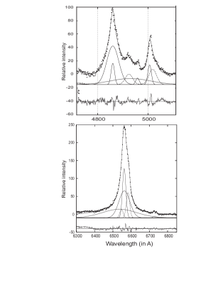
Figure 5: Balmer lines in SDSS J$111603.13+020852.2$ spectrum. Top: H$\beta$ with a highly redshifted H$\beta$ VBLR component; bottom: H$\alpha$ where the VBLR component is not redshifted.

To apply a uniform model of the line fitting procedure, we assumed that Balmer lines have three components from the NLR, ILR and VBLR. We exclude 4 spectra from the sample in which H$\alpha$ line could not be decomposed in this way, so finally our sample contains 133 spectra (from 137) with all Balmer lines which could be analyzed within the $\lambda\lambda$ 6400-6800 Å range. To check this assumption on the rest of the spectra, we examined the corresponding correlations and we found that the luminosities and widths of the NLR, ILR and VBLR components of H$\alpha$ are highly correlated with the same parameters of the NLR, ILR and VBLR components of H$\beta$. This is in favor of our three component decomposition (Table 3). For the 133 objects, which have both H$\beta$ and H$\alpha$ lines, it can be noticed that 16 spectra have large redshifts of the VBLR H$\beta$ component relative to VBLR of H$\alpha$, which causes disagreement and reduces the correlation between the VBLR shifts of the rest of objects. Without these 16 objects, H$\beta$ and H$\alpha$ VBLR components correlate in width and shift, with coefficient of correlation $\sim 0.40$, P $<$ 0.0001. An example of shifts between the H$\alpha$ and H$\beta$ VBLR components is shown in Figure 5. The AGN SDSS J$111603.13+020852.2$ has its VBLR H$\beta$ component redshifted by $\approx$4258 $\mathrm{kms^{-1}}$, while shift of the H$\alpha$ VBLR component is $\approx$-1200 $\mathrm{kms^{-1}}$.

We assume that all narrow lines (and narrow components of the broad lines), originate from the same NLR, and thus expect that these lines will have the same shifts and widths. We therefore took the Gaussian parameters of the shift and width of [O III], [N II], and the NLR components of H$\beta$ and H$\alpha$ to have the same values.

We separately fit lines from the $\lambda\lambda$ 4400-5500 Å range (Fe II lines, [O III], He II and H$\beta$) with 23 free parameters, and lines from the $\lambda\lambda$ 6400-6800 Å range (H$\alpha$ and [N II]) with 8 free parameters. We applied a ${\chi}^{2}$ minimization routine (Popović et al., 2004), to obtain the best fit. Examples of an AGN spectrum fit in both ranges are shown in Figure 6 and Figure 7.

2.4 Line parameters

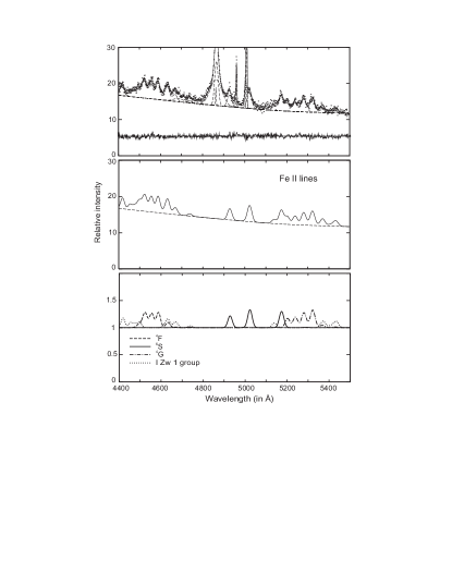
Figure 8: Example of measuring of equivalent widths of the Fe II group of lines. Top: fit spectrum (SDSS J020039.15-084554.9); middle: Fe II lines and continuum; bottom: Fe II lines normalized on the continuum level.

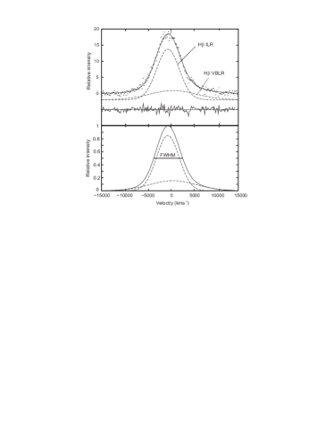
Figure 9: Example of measuring of FWHM; Top: fitted broad H$\beta$ (ILR+VBLR); bottom: FWHM is obtained as width on half maximum of the sum of ILR and VBLR Gaussians.

We compared the shifts, widths, equivalent widths, and luminosities of the lines. The shifts and widths were obtained directly from the fit (parameters of width and shift). Luminosities were calculated using the formulae given in Peebles (1993), with adopted cosmological parameters: $\Omega_{M}$ = 0.27, $\Omega_{\Lambda}$ = 0.73 and $\Omega_{k}$ = 0. We adopt a Hubble constant, $\mathrm{H_{o}=71\ \rm kms^{-1}Mpc^{-1}}$. The continuum luminosity was obtained from the average value of continuum flux measured between 5100 Å ($\lambda\lambda$5095-5100 Å and $\lambda\lambda$5100-5105 Å). Equivalent widths were measured with respect to the continuum below the lines. The continuum was estimated by subtracting all fitted lines from the observed spectra. Then, the line of interest (or the Fe II template), which is fit separately, is added to the continuum. Equivalent widths are obtained by normalizing the lines on continuum level, and measuring their fluxes (see Figure 8). To determine the full width at half maximum (FWHM) of the broad component of the Balmer lines, the VBLR and ILR components from the fit are considered as it is shown in Figure 9. The broad Balmer line (VBLR+ILR) is then normalized on unity, and the FWHM is measured at half of the maximum intensity.

3 Results

3.1 The ratios of Fe II line groups vs. other spectral properties

Some objects have relative intensities of Fe II lines similar to I Zw 1, while others show significant disagreement, which usually shows up as stronger iron emission in the blue bump (mainly $F$ lines) than one in the red bump (mainly $G$ lines), comparing to I Zw 1. That objects could be fitted well with the template model which assumes that relative intensities between the Fe II lines from different line groups ($F$, $S$ and $G$) are different for different objects.

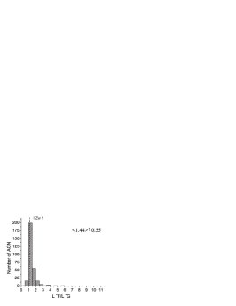
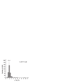
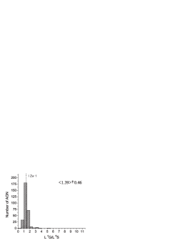
Figure 10: Distribution of the ratios of luminosities of the three Fe II groups ($F$, $S$, and $G$). The mean value and the dispersion of the distribution are given in the plots. We indicate with a dashed vertical line the ratio of Fe II groups we obtained in the I Zw 1 spectrum.

Difference between the relative intensities of the Fe II lines from different parts of iron shelf (blue, red and central) can be illustrated well with histograms of distribution of the Fe II group ratio ($F$/$G$, $F$/$S$ and $G$/$S$) for the sample (Figure 10). The average value of the $F/G$ luminosity ratio is 1.44$\pm$0.55, of the $F/S$ ratio 1.97$\pm$1.05, and of the $G/S$ ratio 1.39$\pm$0.46. We found that the majority of objects have Fe II group ratios close to the average values, but still significant number of objects are showing difference since the intensity ratios of Fe II line groups vary in different objects (see Figure 10). The ratios of the Fe II line groups in I Zw 1 are indicated by the vertical dashed lines ($F/G=1.10$, $F/S=1.56$ and $G/S=1.41$).

We analyzed the flux ratios of the Fe II multiplet groups and the total Fe II flux (see histograms in Figure 11), and we found that lines from multiplets 37 and 38 (group $F$) generally have the largest contribution to the total Fe II emission within the $\lambda\lambda$4400-5500 Å range (about 32%), while group $S$ contributes about 18% and $G$ about 23%. As expected, there are very strong correlations between the equivalent widths of Fe II line groups (Table 4).

Since line intensities and their ratios are indicators of physical properties of the plasma where those lines arise, we have investigated relations among the ratios of Fe II line groups with various spectral properties. A correlation between the FWHM H$\beta$ and the EW Fe II emission has been found previously (Gaskell, 1985; Boroson & Green, 1992; Sulentic et al., 2009). Consequently, one can expect that FWHM H$\beta$ may be connected with the Fe II line group ratios. We therefore investigated correlations between the ratios of the Fe II groups ($F/G$, $F/S$, and $G/S$) and H$\beta$ FWHM. We excluded the three outliers, which have negligible flux for $S$ group. As it can be seen in Figure 12 (first panel) there are different trends for spectra with FWHM H$\beta$ less than and greater than $\sim$3000 $\mathrm{kms^{-1}}$. Therefore, we divided the sample into two sub-samples: 158 objects with FWHM H$\beta$ $<$3000 $\mathrm{kms^{-1}}$ and 141 objects with FWHM H$\beta$ $>$3000 $\mathrm{kms^{-1}}$ (see Figure 12 and Table 5). A similar subdivision of AGN samples was performed by Sulentic et al. (2002, 2009), but for FWHM H$\beta\approx 4000\ \rm kms^{-1}$ as the limiting FWHM of the subdivision. We found that FWHM H$\beta\approx 3000\ \rm kms^{-1}$ is more a appropriate place to divide the objects into two groups, since all objects with strongly redshifted VBLR H$\beta$ component (see Figure 5) belong to the FWHM H$\beta$ $>$3000 $\mathrm{kms^{-1}}$ subsample. Sulentic et al. (2002) also noticed that AGN with FWHM H$\beta$ $>$4000 $\mathrm{kms^{-1}}$, have a larger redshifted VBLR H$\beta$ ($\sim$5000 $\mathrm{kms^{-1}}$).

In Table 5 we present the correlations between the luminosity ratios of the Fe II line groups and other spectral properties such as: FWHM H$\beta$, Doppler width of H$\beta$ broad components, width and shift of iron lines and continuum luminosity ($\mathrm{L_{\lambda 5100}}$). They are examined for the total sample and for two sub-samples, divided according to FWHM H$\beta$, and denoted in Table 5 as (1) for FWHM H$\beta$ $<$3000 $\mathrm{kms^{-1}}$ and (2) for H$\beta$ FWHM $>$3000 $\mathrm{kms^{-1}}$.

We found a difference in the correlations for those two sub-samples. For the H$\beta$ FWHM $>$ 3000 $\mathrm{kms^{-1}}$ sub-sample (2) all three ratios ($F/G$, $F/S$ and $G/S$) increase as H$\beta$ width increases. On the other hand, for the H$\beta$ FWHM $<$ 3000 $\mathrm{kms^{-1}}$ sub-sample no correlation is observed between these properties.

The observed correlation between the $G/S$ group ratio and H$\beta$ FWHM may be caused by intrinsic reddening since reddening increases as objects get more edge-on (Gaskell et al., 2004) and the H$\beta$ FWHM also increases (Wills & Browne, 1986). However, this cannot explain the $F/G$ and $F/S$ correlation with H$\beta$ FWHM, and also, a strong influence of reddening on the $G/S$ ratio is not expected because of the close wavelengths of lines from those groups.

We also studied correlations between continuum luminosity ($\mathrm{L_{\lambda 5100}}$) and Fe II group ratios, since these may indicate excitation processes in the emitting region. We found that the $F/G$ and $F/S$ ratios decrease in objects where the continuum level is higher. Observed correlations are stronger for H$\beta$ FWHM $<$ 3000 $\mathrm{kms^{-1}}$ sub-sample ($F/G$ vs. $\mathrm{L_{\lambda 5100}}$: $r=-0.51$, $P<0.0001$ and $F/S$ vs. $\mathrm{L_{\lambda 5100}}$: $r=-0.41$, $P<0.0001$). The ratio of $G/S$ seems not to be dependent on continuum luminosity.

These correlations are the opposite of what would be expected from reddening, since reddening decreases with luminosity (Gaskell et al., 2004). There are a few effects that could destroy expected reddening effect: (i) incorrect continuum subtraction, (ii) host galaxy fraction which depends on the Eddington ratio and (iii) different contribution of starlight in SDSS fiber which depends on the luminosity of the host galaxy and the redshift (see Gaskell and Kormendy, 2009). There is a small possibility that these effects are important. As we already noted, the error-bar in the continuum subtraction is smaller than 5%. Also, we examined if the host galaxy contribution have influence on considered correlations. We found no correlations between the host galaxy fraction (determined in $\lambda$5100 Å) and Fe II group ratios. The correlations appear instead to be connected with a weaker Baldwin effect for F group (see Table 7).

We also investigated the correlation of the log(L H$\alpha$/L H$\beta$) with ratios of Fe II groups. We found correlations with $F/G$ ($r=-0.36$, $P<0.0001$) and with $F/S$ ratio ($r=-0.34$, $P<0.0001$), but there is no correlation with $G/S$ (Figure 13, Table 6), i.e., between ratio of red and central part. There is possibility that these correlations are caused by intrinsic reddening.

3.2 Connection between kinematical properties of Fe II lines and Balmer lines (H$\alpha$ and H$\beta$)

We assume that broadening of the lines arise by Doppler effect caused by random velocities of emission clouds, and that shifts of lines are a consequence of systemic motions of the emitting gas. We therefore studied the kinematical connection among emission regions by analyzing relationships between their widths and shifts obtained from our best fits.

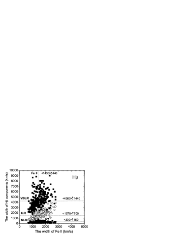
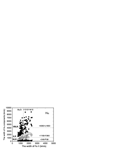
Figure 14: The widths of the Fe II lines compared to the widths of the H$\beta$ (left) and H$\alpha$ (right) components. On the X-axis are the widths of Fe II, and on Y-axis are the widths of the NLR (triangles), ILR (circles), and VBLR (squares) components of H$\beta$ (H$\alpha$). The dotted vertical line shows the average value of Fe II widths, while the dotted horizontal lines show the average values of the H$\beta$ (H$\alpha$) components. The average value of for the Fe II lines is the same as or very close to the average width value of the ILR components of H$\beta$ and H$\alpha$.

The Doppler widths of Fe II and Balmer lines (H$\beta$ and H$\alpha$) are compared in Figure 14. On X-axis we present Fe II width and on the Y-axis the widths of the H$\beta$ (first panel) and H$\alpha$ (second panel) components. The widths of the NLR components are denoted by triangles, the ILR components with circles, and the VBLR components with squares. Dotted lines show the average values of the widths: vertical lines for Fe II components and horizontal lines for H$\beta$ (or H$\alpha$). For the sample of 302 AGN (first panel) the average value of Fe II width and dispersion of the sample are $1430\pm 440$ $\mathrm{kms^{-1}}$, while the average values for H$\beta$ components are: $300\pm 150$ $\mathrm{kms^{-1}}$ (NLR), $1570\pm 700$ $\mathrm{kms^{-1}}$ (ILR) and $4360\pm 1440$ $\mathrm{kms^{-1}}$ (VBLR). For the selected sample of 133 AGNs which have the H$\alpha$ line in the spectra (second panel), the averaged value of the Fe II width is $1310\pm 410$ $\mathrm{kms^{-1}}$ and for the H$\alpha$ components: $240\pm 90$ $\mathrm{kms^{-1}}$ (NLR), $1160\pm 560$ $\mathrm{kms^{-1}}$ (ILR) and $4060\pm 1650$ $\mathrm{kms^{-1}}$ (VBLR). It is obvious that the averaged Fe II width ($\sim 1400$ $\mathrm{kms^{-1}}$) is very close to the average widths of the ILR H$\beta$ and H$\alpha$ components (1568 $\mathrm{kms^{-1}}$ and 1156 $\mathrm{kms^{-1}}$ respectively), while the averaged widths of NLR and VBLR components are significantly different from the Fe II width.

Relationships among the widths of the Fe II and ILR components are also presented in Figure 15 (Table 7). The correlation between the Fe II width and the width of H$\alpha$ ILR is $r=0.77$, $P<0.0001$, and between the Fe II width and the H$\beta$ ILR width it is $r=0.73$, $P<0.0001$. We also found a correlation between the widths of Fe II and the VBLR ($r=0.66$, $P<0.0001$ for the H$\alpha$ VBLR, and r=0.45, $P<0.0001$ for H$\beta$ VBLR).

Relationships between the shifts of Fe II and H$\alpha$ and H$\beta$ components were also considered (Table 7). We found correlations with the shifts of the H$\alpha$ ILR ($r=0.30$, $P=0.0004$) and the H$\beta$ ILR component ($r=0.39$, $P<0.0001$), but no correlation between the shift of Fe II and the shifts of other H$\alpha$ and H$\beta$ components.

We found that Fe II lines tend to have an averaged redshift of 270$\pm$180 $\mathrm{kms^{-1}}$ with respect to the transition wavelength, and with respect to narrow lines 100$\pm$240 $\mathrm{kms^{-1}}$ (see Figure 16).

3.3 Correlations between the Fe II line groups and other emission lines

Correlations between the luminosity of the Fe II multiplet groups, total Fe II and luminosities of the [N II] and [O III] lines are presented in Table 8. In the $L$ [N II] vs. $L$ Fe II plot, seven outliers are observed with negligible [N II]. They are probably caused by an underestimate in the fit of the [N II] lines due to the blending with the H$\alpha$ line. Without these outliers, correlation is $\sim 0.70$, P$<$0.0001. There is no correlation between $L$ [N II]/$L$ [O III] vs. $L$ Fe II.

We analyzed relationships among the luminosities of the Fe II line groups and the NLR, ILR and VBLR H$\alpha$ components (Table 8). All three H$\alpha$ components are correlated with the Fe II line groups. Correlations are stronger with the ILR and VBLR components than with the NLR components. The same analysis was carried out for the luminosities of Fe II line groups and the NLR, ILR and VBLR components of H$\beta$ (Table 8). NLR component of H$\beta$ also has a weaker correlation with Fe II lines (r$\sim$0.60, P$<$0.0001) than broad H$\beta$ components (r$\sim$0.90, P$<$0.0001).

We also investigated the anti-correlations between EW Fe II and EW [O III], and between EW Fe II and EW [O III]/EW H$\beta$ (Boroson & Green, 1992). We confirmed the existence of these relationships in our sample, with Fe II lines separated into $F$, $S$, and $G$ line groups (Figure 17, Table 9). A difference from Boroson & Green (1992), who measured the equivalent widths of all lines referring to the continuum level at the $\lambda 4861$ Å, is that we calculated the equivalent widths by estimating the continuum below all the Fe II lines considered (see Figure 8). Note also that Boroson & Green (1992) used mainly measurements from lines from multiplets 37 and 38.

We found a correlation between total EW Fe II and EW [O III] $r=-0.39$, $P<0.0001$. The correlation coefficient was significantly lower for the lines obtained from I Zw 1 ($r=-0.20$, $P=0.0006$) than for the other three groups (see Table 9). We also analyzed relationships between EW Fe II line groups and EW [O III]/EW H$\beta$. For total EW Fe II we found r= - 0.46, P$<$0.0001 (Figure 17, right), but for lines from I Zw 1 group r= - 0.28, P$<$0.0001.

No significant correlations were found between EW Fe II and EW [N II] lines (Table 9).

We also investigated whether there were any trends between equivalent widths of Fe II $F$, $S$, $G$ line groups and equivalent widths of NLR, ILR and VBLR H$\alpha$ and H$\beta$ components (Table 9). We found no significant correlations.

The correlations between EW Fe II and the Doppler widths of H$\beta$ components are also considered (Table 10). As was expected, an inverse correlation was found between EW Fe II and the widths of the broad H$\beta$ components (ILR and VBLR, as well as for the H$\beta$ FWHM, $r\sim-0.30$, $P<0.0001$). These correlations are part of EV 1. But, contrary to this, we found a positive correlation ($r=0.30$, $P<0.0001$) between the EW Fe II and the width of NLR component.

3.4 Relations among emission line strength and continuum luminosity

In Sec 3.3. we have confirmed the anti-correlation EW Fe II vs. EW [O III] (also EW Fe II vs. EW [O III]/EW H$\beta$). To try to understand the underlying physics which governs this anti-correlation, we examined its dependence of the continuum luminosity and redshift.

Because of selection effects, cosmological redshift, $z$, and continuum luminosity are highly correlated in our sample, so it is difficult to clearly distinguish which influence dominates in some correlations. Since our sample has a more uniform redshift distribution than continuum luminosity distribution (see Figure 2), we binned equivalent widths of the [O III] and Fe II lines within the $z=0$ – 0.7 range, using a $\Delta z=0.1$ bin size. The binned data are presented in Figure 18. It can be seen that as redshift increases in the $z<0.4$ range, EW Fe II also increases, but EW [O III] decreases (Figure 18). For $z>0.4$, the trend is not so obvious, probably due to the larger scatter of the data at higher redshifts.

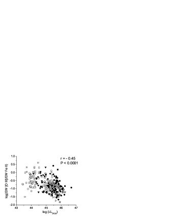
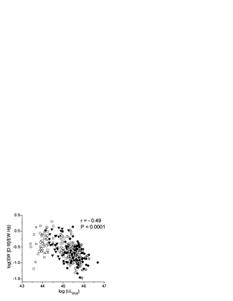
Figure 19: First panel: EW [O III]/EW Fe II ratio vs. continuum luminosity ($\lambda L_{5100}$); second panel: the same for EW [O III]/EW H$\beta$ ratio. Objects with redshift within range z$<$0.1 are denoted with open squares, 0.1$<$z$<$0.2 with filled triangles, 0.2$<$z$<$0.3 with open circles, 0.3$<$z$<$0.4 with filled squares, 0.4$<$z$<$0.5 with open triangles, 0.5$<$z$<$0.6 with filled circles and 0.6$<$z$<$0.7 with stars. [O III] includes only the $\lambda$5007 Å component.

We derived correlations coefficients for the ratios of the [O III], Fe II and H$\beta$ lines and L_λ5100 (also with redshift, see Figure 19, Table Analysis of optical Fe II emission in a sample of AGN spectra). A significant anti-correlation was found for the ratio of EW [O III]/EW Fe II vs. L_λ5100 and for EW [O III]/EW Fe II vs. $z$ ($r=-0.46$, $P=0$ and $r=-0.48$, $P=0$, respectively). We found that the ratios of EW [O III]/EW H$\beta$ and EW H$\beta$ NLR/EW Fe II also decrease as L_λ5100 (redshift) increases. As in the previous case, the difference between the P–values for correlation with L_λ5100 and with $z$ is very small, so we cannot tell which effect dominates. In contrast to this, for EW H$\beta_{\mathrm{total}}$/EW Fe II vs. L_λ5100, no significant trend is observed, but for EW H$\beta_{\mathrm{total}}$/EW Fe II vs. $z$, there is a weak correlation ($r=0.28$, $P=$ 1.3E-6).

Because of discrepancies in the properties observed between sub-samples within different H$\beta$ FWHM ranges (see Sec 3.1), we analyzed the relationships separately for the sub-samples with FWHM H$\beta<$3000 $\mathrm{kms^{-1}}$ and FWHM H$\beta>$3000 $\mathrm{kms^{-1}}$. It will be noticed that, in general, all the correlations considered are stronger for the FWHM H$\beta>$3000 $\mathrm{kms^{-1}}$ sub-sample than for spectra with narrower H$\beta$ lines (see Table Analysis of optical Fe II emission in a sample of AGN spectra). The only exception is the correlation of EW H$\beta$ NLR/EW Fe II vs. L_λ5100, which is more significant for the FWHM H$\beta<$3000 $\mathrm{kms^{-1}}$ subsample.

It is interesting to connect these anti-correlations (EW Fe II vs. EW [O III] and considered ratios vs. L_λ5100) with the Baldwin effect. Baskin & Laor (2004) confirmed a correlation between the Baldwin effect and some of the emission parameters which define Eigenvector 1 correlations (which are related to EW [O III] - EW Fe II anti-correlation). Also, it has been found that the [O III] lines show strong Baldwin effect (Dietrich et al., 2002). On the other hand, no Baldwin effect has been noticed for the optical Fe II and H$\beta$ lines (Dietrich et al., 2002), or even an inverse Baldwin Effect has been reported: Croom et al. (2002) found an inverse Baldwin effect in H$\beta$ and Netzer & Trakhtenbrot (2007) found one for both H$\beta$ and optical Fe II lines.

Because of this, we examined the dependence of the equivalent widths of Fe II, H$\beta$ and [O III] lines vs. L_λ5100 and $z$ in our sample. Since H$\beta$ is decomposed in NLR, ILR and VBLR and the iron lines are separated in the groups they can be considered in more detail. Also, we performed separate analyses for the sub-samples with different H$\beta$ FWHM ranges (Table Analysis of optical Fe II emission in a sample of AGN spectra).

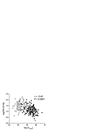
Figure 20: The Baldwin effect is significant for the [O III] lines (first panel), while an inverse Baldwin effect is detected for the optical Fe II lines (second panel). Symbols have the same meaning as in Figure 19.

Analyzing the total sample (i.e., the whole H$\beta$ FWHM range), it is obvious that Fe II lines show an inverse Baldwin effect, which is specially strong for the central ($r=0.33$, $P<0.0001$) and red part ($r=0.44$, $P<0.0001$) of the Fe II shelf ($S$ and $G$ groups), as well as for the group of lines from I Zw 1 ($r=0.32$, $P<0.0001$). The correlation of total Fe II vs. L_λ5100 is presented in Figure 20. What is interesting is that a strong inverse Baldwin effect is not observed for the $F$ lines (blue part) ($r=0.16$, $P=0.004$). In the relationship between H$\beta$ components and continuum luminosity for total sample, no trend is observed for broad H$\beta$ (ILR and VBLR), but it can be noticed that the narrow H$\beta$ component anti-correlates with continuum luminosity ($r=-0.36$, $P<0.0001$), – i.e. they show a Baldwin effect – as well as the [O III] lines, for which the previously found trend is confirmed ($r=-0.43$, $P<0.0001$ – see Figure 20).

If we compare these correlations with the corresponding correlations with redshift, it is obvious that the iron lines (total Fe II and the multiplet groups) correlate more strongly with redshift than with luminosity. In the case of other lines we consider, the difference between the correlations with L_λ5100 and $z$, is not so significant. Generally, it seems that the lines which show an inverse Baldwin effect (Fe II and H$\beta$ VBLR) correlate more significantly with redshift than with luminosity, while the lines which show a (normal) Baldwin effect ([O III] and H$\beta$ NLR) have more significant correlations with continuum luminosity.

We find that the coefficients of correlations between the EWs of lines and the continuum luminosity (and $z$) depend on the H$\beta$ FWHM range of the sub-sample. It seems that continuum luminosity affects iron lines and H$\beta$ more for the subsample with narrower H$\beta$ line (FWHM H$\beta<$3000 $\mathrm{kms^{-1}}$). In that sub-sample all Fe II groups show a stronger inverse Baldwin effect, H$\beta$ NLR decreases more strongly with an increase in continuum luminosity, and an inverse Baldwin effect is also observed for H$\beta$ VBLR ($r=0.41$, $P<0.0001$). This is not seen in the FWHM H$\beta>$3000 $\mathrm{kms^{-1}}$ sub-sample. In contrast with this the Baldwin effect is stronger in the [O III] lines for the FWHM H$\beta>$3000 $\mathrm{kms^{-1}}$ subsample.

4 Discussion

From our analysis of optical Fe II lines ($\lambda\lambda$ 4400-5400 Å), we can try to investigate physical and kinematical characteristics of the Fe II emitting region in AGN as well as the connection between the Fe II and other emission regions. We have investigated above correlations between the Fe II emission properties and some spectral features. Correlations of the Fe II lines were considered separately for different multiplet groups, which enable more detailed analysis. Here we give some discussion of the results we have obtained.

4.1 The Fe II line group ratios – possible physical conditions in the Fe II emitting region

Although we used very simple approximations to calculate the intensities of the observed Fe II lines, we found that the calculated intensities can satisfactorily fit the Fe II shelf within $\lambda\lambda$ 4400-5500 Å range. This approach is very simplified, but in some cases, it enables better fit than much more complicated theoretical models (see Appendix B). We included excitation temperature in calculation and found that it is in the most cases around 10000 K (9646$\pm$2143 K), see Figure 4. Roughly estimated temperature of the Fe II emitting region from our fitting (assumed template) is in a good agreement with the prediction earlier given in literature ($\sim$7000 K, Joly, 1987).

We found that the most intensive emission in the optical part arises in transitions with the lower term b${\ }^{4}F$ (multiplets 37 and 38). We also considered the ratios of multiplet groups. The line ratios may indicate some physical properties. For example, it has been shown that the Balmer line ratios are velocity dependent in AGN (see e.g. Shuder, 1982, 1984; Crenshaw, 1986; Stirpe, 1990, 1991; Snedden & Gaskell, 2007) and this is probably related to a range of physical conditions (electron temperature and density) and to the radiative transfer effects (see e.g. Popović, 2003, 2006). In general, the ratios between F, G and S groups indicate the ratio between the blue, red and central part of the Fe II shelf around H$\beta$ lines. As can be seen in Table 5, there is correlation between $F/G$, $F/S$ and $G/S$ ratios vs. FWHM of H$\beta$ line. It is interesting that this correlation is not present when we consider the cases where FWHM(H$\beta$)$<$ 3000 $\rm kms^{-1}$. We should note here that for the case FWHM(H$\beta$)$<$ 3000 $\rm kms^{-1}$ we had only $\Delta$FWHM(H$\beta$)$\approx$2000 $\mathrm{km\ s^{-1}}$ and this may affect the obtained results. As we mentioned above, the separation of the sample into two sub-samples according to the H$\beta$ FWHM is similar as given in Sulentic et al. (2009, and reference therein). It seems that the characteristics of the Pop A (FWHM H$\beta<$4000$\mathrm{kms^{-1}}$) and B (FWHM H$\beta>$4000$\mathrm{kms^{-1}}$) of AGN (as proposed by the above-mentioned authors) can be recognized in the Fe II line ratios: namely, the correlations and trends observed in Table 5 indicate that the ratios of blue and red (as well as blue and central) parts of Fe II shelf, anti-correlate with continuum luminosity more strongly in Pop A than in Pop B. Also, for Pop B, all considered flux ratios (F/G, F/S and G/S) increase with increasing of H$\beta$ width and with decreasing Fe II shift, while that trend is not observed in Pop A.

The observed anti-correlations of $F/G$ and $F/S$ ratios vs. L_λ5100 could be affected by the differing degrees of inverse Baldwin effect observed for the Fe II lines from the three line groups since the equivalent widths of the $S$ and $G$ groups increase more significantly with $L_{\lambda 5100}$ ($r=0.33$ and $r=0.43$, $P<0.0001$, respectively), than those of the $F$ group ($r=0.16$, $P=0.04$, see Table Analysis of optical Fe II emission in a sample of AGN spectra). Note here that the ratio of $G/S$ does not correlate with the continuum. Also, since the inverse Baldwin effect for the $S$ and $G$ groups is stronger for the FWHM H$\beta<$3000 $\mathrm{kms^{-1}}$ sub-sample, the correlations of $F/G$ and $F/S$ vs. L_λ5100 are stronger for FWHM H$\beta<$3000 $\mathrm{kms^{-1}}$ one (Table 5).

From the above-mentioned correlations, we can ask some intriguing questions about the physical conditions and processes in the Fe II emitting region: (1) which processes cause the increase of Fe II equivalent width with increasing L_λ5100? Note that the equivalent widths of the majority of other emission lines in AGN spectra decrease with increasing L_λ5100 (see Dietrich et al., 2002); (2) why is the inverse Baldwin effect correlation lower for the $F$ group comparing to the $S$ and $G$ groups? and (3) what causes that inverse Baldwin effect for Fe II (in $S$ and $G$) to be more significant in the sub-sample with FWHM H$\beta<$3000 $\mathrm{kms^{-1}}$, than in one with broader H$\beta$ line? Answering some of these questions may lead to a better understanding of the complex Fe II emitting region.

4.2 Location of the Fe II emitting region

Marziani & Sulentic (1993) and Popović et al. (2004) noted earlier that Fe II lines may originate in the intermediate-line region, which may be the transition from the torus to the BLR. Recently, other authors also found that the optical Fe II emission may arise from a region in the outer parts of the BLR or several times larger than the H$\beta$ one (Hu et al., 2008a; Kuehn et al., 2008; Popović et al., 2004, 2007, 2009; Gaskell et al., 2007).

To explore the kinematics of the Fe II emitting region, which may indicate the location of the Fe II emission, we compared the derived widths and shifts of the Fe II and the H$\beta$ and H$\alpha$ components. As can be seen in Figure 14 and Figure 15, there is an indication that Fe II emitting region is located as the IL-emitting region. Moreover, the correlation between the Doppler widths of the Fe II and IL regions is significantly higher than for the VBLR and NLR. There is no significant correlation between the Doppler widths of the Fe II and NL regions ($r=0.01$, $P=0.87$ for H$\alpha$, $r=0.05$, $P=0.40$ for H$\beta$), but there is a correlation between the Fe II and VBLR regions ($r=0.66$, $P<0.0001$ for H$\alpha$, $r=0.45$, $P<0.0001$ for H$\beta$). This may indicate that one more component of the Fe II lines is arising from the VBLR. Note here that, due to the complex Fe II template, we assumed only one component for each Fe II line (see Sect. 2.2). The reasonable fits of the Fe II shelf indicate that, the VBLR component of Fe II should be significantly weaker than the ILR one.

These indications are also supported by the correlation between the shift of the Fe II lines and the ILR components of H$\alpha$ and H$\beta$. The distribution of the Fe II line shifts is shown in Figure 16. The shift is obtained with respect to the transition wavelength (Figure 16, left) and with respect to the narrow lines (Figure 16, right). We found that Fe II lines are slightly redshifted, which is in agreement with the results of Hu et al. (2008a). But in this case, the average value of the Fe II shift relative to the transition wavelength is $270\pm 180$ $\mathrm{kms^{-1}}$, while the average value of the Fe II shift with respect to the narrow lines is $100\pm 240$ $\mathrm{kms^{-1}}$. This implies a significantly smaller redshift than found in Hu et al. (2008a). A slightly redshifted Fe II emission may indicate that Fe II lines arise in an inflowing region (see Gaskell, 2009).

4.3 EW Fe II vs. EW [O III] anti-correlation

One of the problems mentioned in the introduction is the anti-correlation between the equivalent widths of the [O III] and Fe II lines which is related to EV1 in the analysis of Boroson & Green (1992). Some physical causes proposed to explain Eigenvector 1 correlations are: (a) Eddington ratio L/$\mathrm{L_{Edd}}$ (Boroson & Green, 1992; Baskin & Laor, 2004), (b) black hole mass $M_{BH}$, and (c) inclination angle (Miley & Miller, 1979; Wills & Browne, 1986; Marziani et al., 2001). Wang et al. (2006) also suggested that EV1 may be related to AGN evolution.

To try to understand the EW Fe II vs. EW [O III] anti-correlation, we examined its relationship to continuum luminosity and redshift (see Sec 3.4, Table Analysis of optical Fe II emission in a sample of AGN spectra). We found an anti-correlation between the EW [O III]/EW Fe II ratio and L_λ5100. Also, we examined the relations of equivalent widths of Fe II and [O III] lines vs. L_λ5100. We confirmed a strong Baldwin effect for [O III] lines, and an inverse Baldwin effect for EW Fe II lines, i.e. we found that as continuum luminosity increases, EW Fe II also increases, but EW [O III] decreases. This implies that the EW Fe II - EW [O III] anti-correlation may be influenced by Baldwin effect for [O III] and an inverse Baldwin effect for Fe II lines. Also, in our analysis we found that the strength of the Baldwin effect depends on the H$\beta$ FWHM of the sample (see Table Analysis of optical Fe II emission in a sample of AGN spectra). Note that H$\beta$ FWHM is one of the parameters in Eigenvector 1. As it is mentioned in the introduction (Sec 1), some indications of connection between Baldwin effect and EV1 have been given in Baskin & Laor (2004) and Dong et al. (2009). Ludwig et al. (2009) found that the significance of the EV1 relationships is a strong function of continuum luminosity, i.e., the relationships between EW Fe II, EW [O III] and H$\beta$ FWHM can be detected only in a high-luminosity sample of AGNs (log$\lambda L_{5100}>44.7$), as well as a Baldwin effect for [O III] lines

The origin of the Baldwin effect is still not understood and is a matter of debate. The increase of the continuum luminosity may cause a decrease of the covering factor, or changes in the spectral energy distribution (softening of the ionizing continuum) which may result in the decrease of EWs. The inclination angle may also be related to Baldwin effect (for review see Green et al., 2001). The physical properties which are usually considered as a primary cause of the Baldwin effect are: M_BH (Warner et al., 2003; Xu et al., 2008), L/L$\odot$ (Boroson & Green, 1992; Baskin & Laor, 2004), and changes in gas metalicity (Dietrich et al., 2002). Also, a connection between Baldwin effect and AGN evolution is possible (see Green et al., 2001).

We investigated if the correlations observed between L_λ5100 and the equivalent widths of the lines (as well as EW [O III] vs. EW Fe II) are primarily caused by evolution. Since continuum luminosity is strongly correlated with cosmological redshift in our sample, it is difficult to separate luminosity from evolutionary effect. The exception are correlations of EW Fe II vs. $z$, as well as the ratio EW H$\beta_{\mathrm{total}}$/EW Fe II vs. $z$, which are significantly stronger than correlations of the same quantities with L_λ5100. This implies that inverse Baldwin effect of Fe II may be governed first of all by an evolutionary effect. This result is in agreement with results of Green et al. (2001).

5 Conclusions

In this paper we have investigated characteristic of the Fe II emission region, using the sample of 302 AGN from SDSS. To analyze the Fe II emission, an Fe II template was constructed by grouping the strongest Fe II multiplets into three groups, according to the atomic properties of transitions.

We have investigated the correlations of these Fe II groups and their ratios with other lines in spectra. In this way, we tried to find some physical connection between the Fe II and other emitting regions, as well as to connect Fe II atomic structure with the physical properties of the emitting plasma.

We also investigated the kinematical connection between Fe II and the Balmer emission region. In particular the anti-correlation of EW Fe II – EW [O III] and its possible connection with AGN luminosity and evolution were analzed. From our investigation we can outline the following conclusions:

1. We have proposed here an optical Fe II template for the $\lambda\lambda$4400-5500 Å range, which consists of three groups of Fe II multiplets, grouped according to the lower terms of transitions ($F$, $S$ and $G$), and an additional group of lines reconstructed from the I Zw 1 spectrum. We found that template can satisfactorily fit the Fe II lines. In spectra in which Fe II emission lines have different relative intensities than in I Zw 1, this template fit better than empirical and theoretical templates based on I Zw 1 spectrum (see more in Appendix B). Using this template, we are able to consider different groups of transitions which contribute to the blue, central and red part of Fe II shelf around the H$\beta$+[O III] lines.

2. We find that the ratios of different parts of the iron shelf ($F/G$, $F/S$, and $G/S$) depend of some spectral properties such as: continuum luminosity, H$\beta$ FWHM, shift of Fe II, and $\mathrm{H\alpha}$/$\mathrm{H\beta}$ flux ratio. Also, it is noticed that spectra with H$\beta$ FWHM greater and less than $\sim$3000 $\mathrm{kms^{-1}}$ have different properties which is reflected in significantly different coefficients of correlation between the parameters.

3. We found that the Fe II emission is mainly characterized with a random velocity of $\sim$1400 $\mathrm{kms^{-1}}$ that corresponds to the ILR origin, which is also supported by the significant correlation between the width of Fe II and H$\alpha$, H$\beta$ ILR widths. This is in agreement with the previous investigations (Popović et al., 2004; Hu et al., 2008a; Kuehn et al., 2008), but unlike the earlier investigations, we found a slight correlation with the width of VBLR. Therefore, it is possible that Fe II is partly produced in the VBLR and cannot be resolved from continuum luminosity. Also, we found that the Fe II lines are slightly redshifted relative to the narrow lines ($\sim$ 100 $\mathrm{kms^{-1}}$) (see Figure 16).

4. The Balmer lines were decomposed into NLR, ILR and VBLR components and relationships among H$\beta$ components and some spectral properties were investigated. We found a positive correlation between the width of narrow lines and EW Fe II ($r=0.30$, $P<0.0001$), while the width of the broad H$\beta$ components anti-correlates with EW Fe II. Also, we found a Baldwin effect in the case of H$\beta$ NLR component, while the ILR component showed no correlation with continuum luminosity, and VBLR component shows an inverse Baldwin effect for the FWHM $<$ 3000 $\mathrm{kms^{-1}}$ subsample.

5. We confirm in our sample the anti-correlation between EW Fe II and EW [O III] which is related to Eigenvector 1 (EV1) in Boroson & Green (1992) and we examined its dependence on the continuum luminosity and redshift. We found an inverse Baldwin effect for Fe II lines from the central and red part of the Fe II shelf ($S$ and $G$), but for Fe II lines from blue part ($F$) no correlation was observed. A Baldwin effect was confirmed for the [O III] lines. Since EW Fe II increases, and EW [O III] decreases with increases of continuum luminosity (and also the trend of decreasing of EW [O III]/EW Fe II ratio with luminosity is obvious), the observed EW Fe II vs. EW [O III] anti-correlation is probably due to the same physical reason which causes the Baldwin effect. Moreover, it is observed that the coefficients of correlation due to Baldwin effect depend on H$\beta$ FWHM range of a sub-sample, which also implies the connection between the Baldwin effect and EV1. A decreasing trend is observed for EW [O III]/EW H$\beta$ vs. continuum luminosity.

6. We found that the equivalent width of the Fe II lines, as well as the EW H$\beta_{\mathrm{total}}$/EW Fe II ratio have a stronger correlation with redshift, than with continuum luminosity. This implies that the inverse Baldwin effect of Fe II may be primarily caused by evolution.

Appendix A The sample selection

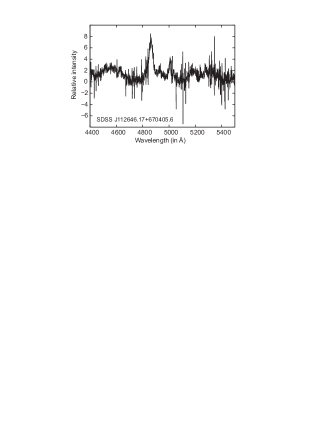
Figure 21: Example of a spectrum rejected because of strong noise which inhibited a precise fit to the iron lines.

Using an SQL search with requirements mentioned in Sec 2.1, we obtained 497 AGN spectra with broad emission lines. From that number, 188 spectra were rejected because of noise in the iron emission line region. An example of rejected spectrum is shown in Figure 21. Also, three spectra were rejected because of bad pixels, and one because of very strong double-peak emission in H$\beta$ (SDSS J154213.91$+$183500.0).

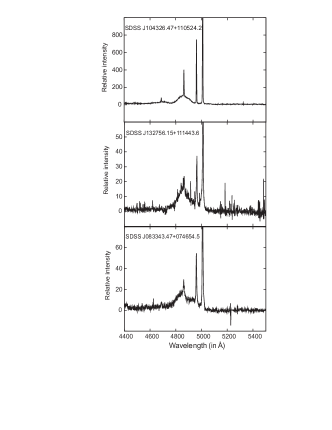
Figure 22: The three spectra with broad H$\beta$ line and without Fe II emission.

Three more spectra with broad H$\beta$ and practically without the Fe II emission were rejected since it was not possible to fit the Fe II lines (SDSS J132756.15$+$111443.6, SDSS J104326.47$+$110524.2 and SDSS J083343.47$+$074654.5). These three spectra are shown in Figure 22. There is also a possibility that in these three objects the Fe II lines are very broad and weak so that they cannot be distinguished from the continuum emission.

The sample contains 302 AGN spectra (table with the SDSS identification and obtained parameters from the best fit is available electronically only, as an additional file at http://www.aob.rs/$\sim$jkovacevic/table.txt).

To test the host galaxy contribution in the selected sample of 302 AGNs, we have compared our sample with the set of AGNs which host galaxy fraction is determined in Vanden Berk et al. (2006). We found 106 common objects. In the case of 48 AGNs (45% of the sample) there is practically no host galaxy contribution (0%), and in the rest of the objects, the contribution of the host galaxy is mainly smaller than 20%.

Appendix B Comparison with other Fe II templates

We compared two Fe II templates (one empirical and one theoretical) with our template. The empirical Fe II template was taken from Dong et al. (2008) using 46 broad and 95 narrow lines identified by Veron-Cetty et al. (2004) in the I Zw 1 spectrum within a $\lambda\lambda$4400-5500 Å range. The Fe II lines were fit with 6 free parameters (the width, shift and intensity for narrow and the width, shift and intensity for broad lines). We also considered the theoretical model from Bruhweiler & Verner (2008) calculated for log[$\mathrm{n_{H}}$/(cm^-3)]=11, [$\xi$]/(1 km s^-1)=20 and log[$\mathrm{\Phi_{H}}$/(cm^-2 s^-1)]=21, since we found that this gave the best fit for those values of physical parameters. With this model, Fe II lines were fit with 3 free parameters (width, shift and intensity).

Figure 23 shows the spectrum of SDSS J020039.15-084554.9, an object in which the iron lines have similar relative intensities to I Zw 1. We fit that spectrum with our template (a), with a template based on line intensities from I Zw 1 (Dong et al., 2008) (b) and with a template calculated by CLOUDY code (Bruhweiler & Verner, 2008) (c). We found that for this object all three templates fit the iron lines well.

In the case of the SDSS J$141755.54+431155.8$, however (Figure 24), the iron lines in the blue bump are slightly stronger compared to those in the red, and our model fit iron emission slightly better than the other two templates. The discrepancy between the blue and red Fe II bumps is especially emphasized in the spectrum of the object SDSS J$111603.13+020852.2$ (Figure 25), which makes a significant difference for comparison with the Fe II properties of I Zw 1 object. In this case, our template shows a small disagreement for the lines whose relative intensity is taken from I Zw 1, but other two models, cannot fit well this type of the Fe II emission. Disagreement is particularly strong in the blue bump (i.e., in the multiplets 37 and 38 of the $F$ group).

Appendix C The relative intensities of Fe II lines

To estimate the relative intensities of Fe II lines within the three groups, we stated that the intensity of a line ($m\to n$) should be proportional to the number of emitters ($N_{m}$)(Osterbrock, 1989; Griem, 1997), i.e. for optically thin plasma (for Fe II lines) one can write: $I_{mn}=const\cdot\frac{A_{mn}}{\lambda_{mn}}\int_{0}^{\ell}N_{m}dx$, where $A_{mn}$ is the probability of the transition, $\lambda_{mn}$ is the transition wavelength, and $\ell$ is the depth of the emitting region.

Of course, the density of emitters can be non-uniform across the region, but we can approximate here that it is uniform, and in the case of non-thermodynamical equilibrium it could be written (Osterbrock, 1989):

$$N_{m}\sim b(T,N_{e})g_{m}\exp{(-E_{mn}/kT)},$$

where b(T,$N_{e}$) represents deviation from thermodynamical equilibrium. In the case of lines which have the same lower level, one may approximate the ratio as (Griem, 1997):

$$\frac{I_{1}}{I_{2}}=\frac{b_{1}(T,N_{e})}{b_{2}(T,N_{e})}{(\frac{\lambda_{2}}{\lambda_{1}})}^{3}\frac{f_{1}}{f_{2}}\cdot\frac{g_{1}}{g_{2}}\cdot e^{-(E1-E2)/kT}$$ (C1)

Assuming that $\frac{b_{1}(T,N_{e})}{b_{2}(T,N_{e})}\approx 1$ we obtained Eq. (1) for estimation of line ratios within one group.

Figure 2: Distribution of continuum luminosity (left) and cosmological redshift (right) in the AGN sample.

Figure 3: An example of removing the continuum from the spectrum of SDSS J$075101.42+29174000.00$; The level of the continuum is determined by interpolating between the chosen points at wavelengths without emission lines (top). The spectrum without continuum emission is shown at the bottom;

Figure 4: The distribution of the excitation temperatures for the sample of 302 AGNs. Temperatures are obtained by fits using Eq. (1). The mean value and dispersion are shown in the Figure.

Figure 6: The spectrum of SDSS J$141755.54+431155.8$ in the $\lambda\lambda$ 4400-5500 Å region: (A) the observed spectra (dots) and the best fit (solid line). (B) H$\beta$ fit with the sum of three Gaussians representing emission from the NLR, ILR and VBLR. The [O III] $\lambda\lambda$4959, 5007 Å lines are fit with two Gaussians for each line of the doublet and He II $\lambda$4686 Å is fit with one broad Gaussian. The Fe II template is denoted with a dashed line, and also represented separately in panel C (bottom).

Figure 7: Fits of SDSS J$141755.54+431155.8$ in the $\lambda\lambda$ 6400-6800 Å region: H$\alpha$ is fit with the sum of three Gaussians which represent emission from NLR, ILR and VBLR and [N II] $\lambda\lambda$6548, 6583 Å lines are fit with one Gaussian for each line of doublet. Narrow [N II] lines are denoted with dashed lines.

Figure 11: The distribution of the ratios of total Fe II (4400-5500 Å) and Fe II groups ($F$, $S$ and $G$). The mean value and the dispersion of the distribution are shown.

Figure 12: The relationship between $F/S$ and H$\beta$ FWHM, for total sample (left), sub-sample of H$\beta$ FWHM $<$ 3000 $\mathrm{kms^{-1}}$ (middle) and the sub-sample of H$\beta$ FWHM $>$ 3000 $\mathrm{kms^{-1}}$ (right).

Figure 13: The relationship between Fe II group ratios and the Balmer decrement.

Figure 15: The correlation between the widths of Fe II and the H$\beta$ ILR (left), H$\alpha$ ILR (middle) and H$\alpha$ VBLR components (right). In all cases, correlations are observed ($r=0.67$, 0.72, 0.62), indicating kinematical connection between these emission regions.

Figure 16: Distribution of the Fe II shift with respect to the transition wavelength (left) and distribution of the Fe II shift with respect to the [O III] lines (right).

Figure 17: Relationship between the EW [O III] $\lambda$5007 Å vs. EW Fe II (left) and EW [O III]/EW H$\beta$ vs. EW Fe II (right).

Figure 18: Relationship between the equivalent widths, EW [O III]$\lambda$ 5007 Å and EW Fe II, binned for cosmological redshift. The error bars are the dispersions in each sub-sample within different redshift bins.

Figure 25: Examples of fits to SDSS J$111603.13+020852.2$: with our template (a), with the empirical template of Dong et al. (2008) (b) and with the theoretical template of Bruhweiler & Verner (2008) (c). In this object iron emission is much stronger in blue than in red bump. Our template show disagreement for lines whose relative intensity is taken from I Zw 1, but other the three wavelength regions based on our three line groups fit the observed Fe II well. The other two models cannot fit this kind of Fe II emission well.

Table 1: A list of the 35 strongest Fe II lines within the $\lambda\lambda$ 4400-5500 Å region used to calculate the Fe II template. In the first column are wavelengths (in air), in the second multiplet numbers (Giridhar & Ferro, 1995), in the third are terms of transitions, in the fourth are $gf$ values used for the template calculation, in the fifth are the references for the source of oscillator strengths, and in the 6th-8th columns are relative intensities, calculated for T=5000 K, 10000 K and 15000 K. Intensities of lines from the $F$, $S$ and $G$ groups are normalized to intensities of the $\lambda$4549.474 Å, $\lambda$5018.44 Å,  and $\lambda$5316.6 Å lines (respectively).

Wavelength	Multiplet	Transition	gf	ref.	Relative intensity
					T=5000 K	T=10000 K	T=15000 K
4472.929	37	b${\ }^{4}F_{5/2}$ - z${\ }^{4}F^{o}_{3/2}$	4.02E-04	1	0.033	0.036	0.037
4489.183	37	b${\ }^{4}F_{7/2}$ - z${\ }^{4}F^{o}_{5/2}$	1.20E-03	1	0.105	0.110	0.111
4491.405	37	b${\ }^{4}F_{3/2}$ - z${\ }^{4}F^{o}_{3/2}$	2.76E-03	1	0.226	0.243	0.249
4508.288	38	b${\ }^{4}F_{3/2}$ - z${\ }^{4}D^{o}_{1/2}$	4.16E-03	2	0.345	0.367	0.375
4515.339	37	b${\ }^{4}F_{5/2}$ - z${\ }^{4}F^{o}_{5/2}$	3.89E-03	2	0.333	0.348	0.353
4520.224	37	b${\ }^{4}F_{9/2}$ - z${\ }^{4}F^{o}_{7/2}$	2.50E-03	3	0.235	0.233	0.233
4522.634	38	b${\ }^{4}F_{5/2}$ - z${\ }^{4}D^{o}_{3/2}$	9.60E-03	3	0.827	0.859	0.870
4534.168	37	b${\ }^{4}F_{3/2}$ - z${\ }^{4}F^{o}_{5/2}$	3.32E-04	3	0.028	0.029	0.030
4541.524	38	b${\ }^{4}F_{3/2}$ - z${\ }^{4}D^{o}_{3/2}$	8.80E-04	3	0.075	0.078	0.079
4549.474	38	b${\ }^{4}F_{7/2}$ - z${\ }^{4}D^{o}_{5/2}$	1.10E-02	4	1.000	1.000	1.000
4555.893	37	b${\ }^{4}F_{7/2}$ - z${\ }^{4}F^{o}_{7/2}$	5.20E-03	3	0.477	0.474	0.474
4576.340	38	b${\ }^{4}F_{5/2}$ - z${\ }^{4}D^{o}_{5/2}$	1.51E-03	4	0.136	0.136	0.136
4582.835	37	b${\ }^{4}F_{5/2}$ - z${\ }^{4}F^{o}_{7/2}$	7.80E-04	3	0.070	0.070	0.070
4583.837	38	b${\ }^{4}F_{9/2}$ - z${\ }^{4}D^{o}_{7/2}$	1.44E-02	2	1.420	1.353	1.331
4620.521	38	b${\ }^{4}F_{7/2}$ - z${\ }^{4}D^{o}_{7/2}$	8.32E-04	4	0.080	0.076	0.075
4629.339	37	b${\ }^{4}F_{9/2}$ - z${\ }^{4}F^{o}_{9/2}$	4.90E-03	4	0.497	0.459	0.447
4666.758	37	b${\ }^{4}F_{7/2}$ - z${\ }^{4}F^{o}_{9/2}$	6.02E-04	4	0.060	0.055	0.054
4993.358	36	b${\ }^{4}F_{9/2}$ - z${\ }^{6}P^{o}_{7/2}$	3.26E-04	4	0.041	0.030	0.027
5146.127	35	b${\ }^{4}F_{7/2}$ - z${\ }^{6}F^{o}_{7/2}$	1.22E-04	5	0.016	0.011	0.010
4731.453	43	a${\ }^{6}S_{5/2}$ - z${\ }^{4}D^{o}_{7/2}$	1.20E-03	2	0.025	0.030	0.032
4923.927	42	a${\ }^{6}S_{5/2}$ - z${\ }^{6}P^{o}_{3/2}$	2.75E-02	4	0.656	0.693	0.706
5018.440	42	a${\ }^{6}S_{5/2}$ - z${\ }^{6}P^{o}_{5/2}$	3.98E-02	4	1.000	1.000	1.000
5169.033	42	a${\ }^{6}S_{5/2}$ - z${\ }^{6}P^{o}_{7/2}$	3.42E-02	1	0.929	0.854	0.831
5284.109	41	a${\ }^{6}S_{5/2}$ - z${\ }^{6}F^{o}_{7/2}$	7.56E-04	2	0.022	0.019	0.018
5197.577	49	a${\ }^{4}G_{5/2}$ - z${\ }^{4}F^{o}_{3/2}$	7.92E-03	5	0.532	0.620	0.652
5234.625	49	a${\ }^{4}G_{7/2}$ - z${\ }^{4}F^{o}_{5/2}$	8.80E-03	3	0.615	0.695	0.723
5264.812	48	a${\ }^{4}G_{5/2}$ - z${\ }^{4}D^{o}_{3/2}$	1.08E-03	1	0.075	0.084	0.087
5276.002	49	a${\ }^{4}G_{9/2}$ - z${\ }^{4}F^{o}_{7/2}$	1.148e-02	2	0.861	0.928	0.951
5316.615	49	a${\ }^{4}G_{11/2}$ - z${\ }^{4}F^{o}_{9/2}$	1.17E-02	4	1.000	1.000	1.000
5316.784	48	a${\ }^{4}G_{7/2}$ - z${\ }^{4}D^{o}_{5/2}$	1.23E-03	5	0.089	0.097	0.099
5325.553	49	a${\ }^{4}G_{7/2}$ - z${\ }^{4}F^{o}_{7/2}$	6.02E-04	4	0.044	0.047	0.048
5337.732	48	a${\ }^{4}G_{5/2}$ - z${\ }^{4}D^{o}_{5/2}$	1.28E-04	5	0.009	0.010	0.010
5362.869	48	a${\ }^{4}G_{9/2}$ - z${\ }^{4}D^{o}_{7/2}$	1.82E-03	5	0.142	0.146	0.148
5414.073	48	a${\ }^{4}G_{7/2}$ - z${\ }^{4}D^{o}_{7/2}$	1.60E-04	5	0.012	0.012	0.013
5425.257	49	a${\ }^{4}G_{9/2}$ - z${\ }^{4}F^{o}_{9/2}$	4.36E-04	5	0.035	0.035	0.035

Table 2: List of the lines taken from Kurucz database (http://www.pmp.uni-hannover.de/cgi-bin/ssi/test/kurucz/sekur.html). In first column are wavelengths (in air), in the second oscillator strengths, and in the third relative intensities measured in I Zw 1.

Wavelength	Transitions	gf	Relative intensity
4418.957	y${\ }^{4}G_{5/2}$ - e${\ }^{4}F_{3/2}$	1.45E-02	3.00
4449.616	y${\ }^{4}G_{9/2}$ - e${\ }^{4}F_{7/2}$	2.58E-02	1.50
4471.273	y${\ }^{4}D_{5/2}$ - f${\ }^{4}D_{3/2}$	6.40E-03	1.20
4493.529	y${\ }^{4}G_{10/2}$ - e${\ }^{4}F_{9/2}$	3.74E-02	1.60
4614.551	y${\ }^{6}P_{5/2}$ - ${\ }^{6}D_{7/2}$	2.69E-03	0.70
4625.481	x${\ }^{4}D_{1/2}$ - f${\ }^{4}D_{1/2}$	8.51E-03	0.70
4628.786	x${\ }^{4}D_{5/2}$ - f${\ }^{4}D_{5/2}$	1.83E-02	1.20
4631.873	x${\ }^{4}D_{3/2}$ - f${\ }^{4}D_{3/2}$	1.34E-02	0.60
4660.593	$d^{5}4s^{2}{\ }^{2}G_{7/2}$ - $(4G)sp{\ }^{2}G_{7/2}$	1.15E-03	1.00
4668.923	x${\ }^{4}D_{5/2}$ - f${\ }^{4}D_{7/2}$	3.13E-03	0.90
4740.828	y${\ }^{6}P_{5/2}$ - e${\ }^{6}F_{7/2}$	1.98E-03	0.50
5131.210	y${\ }^{4}P_{5/2}$ - e${\ }^{4}D_{5/2}$	2.13E-03	1.1
5369.190	e${\ }^{4}D_{5/2}$ - ${\ }^{4}D_{5/2}$	1.23E-03	1.45
5396.232	x${\ }^{4}F_{5/2}$ - f${\ }^{4}D_{3/2}$	2.80E-03	0.40
5427.826	b${\ }^{4}G_{11/2}$ - w${\ }^{4}F_{9/2}$	2.17E-02	1.40

Table 3: Correlations between widths, shifts and luminosities of the NLR, ILR and VBLR components of the H$\alpha$ and H$\beta$ lines. The values in brackets are for the sample without the 16 objects with highly redshifted H$\beta$ VBLR components ($>$4000 $\mathrm{kms^{-1}}$). The coefficient of correlation ($r$) is in the second column, the $P$-value which is a measure of significance of the correlation is given in the third column, and in the next columns are the coefficients $A$ and $B$ from the fit with a linear function: $H\beta=A+B\cdot H\alpha$. The slopes are from regressions where $X$ is taken as the independent variable.

correlation (H$\alpha$ and H$\beta$)	r	P	A	B
H$\alpha$ NLR width vs. H$\beta$ NLR width	0.99	$<0.0001$	$6.19\pm 2.81$	$0.97\pm 0.01$
H$\alpha$ ILR width vs. H$\beta$ ILR width	0.91	$<0.0001$	$165.37\pm 43.29$	$0.74\pm 0.03$
H$\alpha$ VBLR width vs. H$\beta$ VBLR width	0.50 (0.42)	$<0.0001$	$1863.15\pm 352.50$	$0.54\pm 0.08$
H$\alpha$ NLR shift vs. H$\beta$ NLR shift	0.97	$<0.0001$	$16.40\pm 3.58$	$0.91\pm 0.02$
H$\alpha$ ILR shift vs. H$\beta$ ILR shift	0.90	$<0.0001$	$-1.86\pm 16.97$	$1.09\pm 0.05$
H$\alpha$ VBLR shift vs. H$\beta$ VBLR shift	0.18 (0.41)	0.041 ($<0.0001$)	$-93.64\pm 45.30$	$0.06\pm 0.03$
L H$\alpha$ NLR vs. L H$\beta$ NLR	0.93	$<0.0001$	$3.40\pm 1.29$	$0.93\pm 0.03$
L H$\alpha$ ILR vs. L H$\beta$ ILR	0.96	$<0.0001$	$1.93\pm 1.08$	$0.97\pm 0.03$
L H$\alpha$ VBLR vs. L H$\beta$ VBLR	0.96	$<0.0001$	$0.70\pm 1.03$	$0.99\pm 0.02$

Table 4: Correlatios between equivalent widths (EW) of the Fe II $F$, $S$ and $G$ multiplet groups. Relationships are fitted with function $Y=A+B\cdot X$. The coefficient of correlations, $r$, the corresponding measure of the significance of correlations, $P$, as well as the $A$ and $B$ coefficients, are shown in the table.

X	Y	r	P	A	B
EW Fe II F	EW Fe II S	0.76	$<0.0001$	$0.21\pm 1.00$	$0.66\pm 0.03$
EW Fe II F	EW Fe II G	0.80	$<0.0001$	$-0.17\pm 1.29$	$0.96\pm 0.04$
EW Fe II S	EW Fe II G	0.83	$<0.0001$	$5.39\pm 0.95$	$0.14\pm 0.04$

Table 5: Correlations between the ratio of Fe II line groups and spectral properties. In the first column is FWHM of broad H$\beta$ (ILR+VBLR), in the second and third columns are the Doppler widths of ILR and VBLR H$\beta$ components, in the fourth and fifth the Doppler width and shift of Fe II lines, and in the eighth column is the continuum luminosity at $\lambda$5100 Å. Correlation coefficients are calculated for total sample, for objects with H$\beta$ FWHM $<$ 3000 $\mathrm{kms^{-1}}$ (1), and with H$\beta$ FWHM $>$ 3000 $\mathrm{kms^{-1}}$ (2). The correlations with $P<0.0001$ are printed in bold print.

		H$\beta$ FWHM	w H$\beta$ ILR	w H$\beta$ VBLR	w Fe II	sh Fe II	log $\lambda L_{5100}$
F/G	r	0.28	0.24	0.29	0.18	- 0.27	- 0.32
	P	7.13E-7	2.49E-5	2.37E-7	0.002	2.75E-6	1.82E-8
(1) F/G	r	- 0.10	- 0.02	0.16	0.001	- 0.10	- 0.51
	P	0.20	0.831	0.046	0.987	0.189	5.72E-12
(2) F/G	r	0.36	0.27	0.31	0.17	- 0.30	- 0.36
	P	1.22E-5	0.001	1.82E-4	0.043	3.31E-4	8.98E-6
F/S	r	0.41	0.26	0.16	0.20	- 0.27	- 0.15
	P	1.95E-13	4.05E-6	0.004	5.47E-4	2.44E-6	0.011
(1) F/S	r	- 0.21	- 0.18	0.07	-0.23	- 0.11	- 0.41
	P	0.009	0.027	0.407	0.004	0.182	7.90E-8
(2) F/S	r	0.59	0.33	0.12	0.25	- 0.29	- 0.18
	P	1.35E-14	5.08E-5	0.157	0.002	5.29E-4	0.035
G/S	r	0.26	0.16	0.03	0.07	- 0.11	0.06
	P	3.92E-6	0.004	0.646	0.213	0.048	0.312
(1) G/S	r	- 0.09	- 0.17	- 0.09	- 0.26	0.003	0.14
	P	0.243	0.036	0.277	0.001	0.965	0.076
(2) G/S	r	0.44	0.28	0.01	0.15	- 0.13	0.006
	P	6.15E-8	8.26E-4	0.867	0.07	0.113	0.935

Table 6: The relationship between log (L H$\alpha$/L H$\beta$) and the ratios of the Fe II groups.

		log (L H$\alpha$/L H$\beta$)
log (F/G)	r	-0.36
	P	$<0.0001$
log (F/S)	r	-0.34
	P	$<0.0001$
log (G/S)	r	0.004
	P	0.962

Table 7: Relationships between the Fe II width and the widths of the NLR, ILR, and VBLR components of the H$\alpha$ and H$\beta$ (left), and the same but for the shifts (right). Relationships are fitted with function $Y=A+B\cdot X$. The coefficient of correlations, $r$, the corresponding measure of the significance of correlations, $P$, as well as the $A$ and $B$ coefficients, are shown in the table.

		w Fe II	Corr.			shift Fe II	Corr.
w H$\alpha$ NLR	r	0.01	No	sh H$\alpha$ NLR	r	0.02	No
	P	0.871			P	0.84
	A	$232.71\pm 27.12$			A	$149.78\pm 8.88$
	B	$0.00\pm 0.02$			B	$0.00\pm 0.02$
w H$\alpha$ ILR	r	0.77	Yes	sh H$\alpha$ ILR	r	0.30	Yes, weak
	P	$<0.0001$			P	0.0004
	A	$-94.35\pm 111.64$			A	$66.10\pm 26.11$
	B	$0.96\pm 0.08$			B	$0.26\pm 0.07$
w H$\alpha$ VBLR	r	0.66	Yes	sh H$\alpha$ VBLR	r	0.01	No
	P	$<0.0001$			P	0.930
	A	$609.84\pm 356.76$			A	$-49.14\pm 44.47$
	B	$2.63\pm 0.26$			B	$0.01\pm 0.12$
w H$\beta$ NLR	r	0.05	No	sh H$\beta$ NLR	r	0.00	No
	P	0.401			P	0.928
	A	$275.84\pm 30.17$			A	$165.22\pm 9.63$
	B	$0.02\pm 0.02$			B	$0.00\pm 0.03$
w H$\beta$ ILR	r	0.73	Yes	sh H$\beta$ ILR	r	0.39	Yes
	P	$<0.0001$			P	$<0.0001$
	A	$-114.23\pm 94.28$			A	$55.32\pm 14.80$
	B	$1.17\pm 0.06$			B	$0.32\pm 0.04$
w H$\beta$ VBLR	r	0.45	Yes	sh H$\beta$ VBLR	r	-0.17	No
	P	$<0.0001$			P	0.003
	A	$2241.03\pm 251.81$			A	$1301.87\pm 96.29$
	B	$1.48\pm 0.17$			B	$-0.83\pm 0.28$

Table 8: Correlations between luminosities ($L$) of the Fe II lines (total Fe II, $F$, $S$ and $G$ line groups) and luminosities of [N II], [O III] and H$\alpha$ and H$\beta$ components. Relationships are fitted with function $Y=A+B\cdot X$. The coefficient of correlations, $r$, and the corresponding measure of the significance of correlations, $P$ are shown in the table.

		log(L Fe II total)	log(L F)	log(L S)	log(L G)	log(L I Zw 1 group)
log(L [N II])	r	0.73	0.72	0.67	0.73	0.72
	P	$<0.0001$	$<0.0001$	$<0.0001$	$<0.0001$	$<0.0001$
log(L [N II]/L [O III])	r	0.06	0.08	0.08	0.10	0.02
	P	0.51	0.38	0.35	0.25	0.84
log(L H$\alpha$ NLR)	r	0.76	0.74	0.71	0.75	0.77
	P	$<0.0001$	$<0.0001$	$<0.0001$	$<0.0001$	$<0.0001$
log(L H$\alpha$ ILR)	r	0.91	0.90	0.84	0.89	0.90
	P	$<0.0001$	$<0.0001$	$<0.0001$	$<0.0001$	$<0.0001$
log(L H$\alpha$ VBLR)	r	0.90	0.89	0.82	0.87	0.90
	P	$<0.0001$	$<0.0001$	$<0.0001$	$<0.0001$	$<0.0001$
log(L H$\beta$ NLR)	r	0.64	0.63	0.61	0.63	0.64
	P	$<0.0001$	$<0.0001$	$<0.0001$	$<0.0001$	$<0.0001$
log(L H$\beta$ ILR)	r	0.93	0.93	0.88	0.92	0.92
	P	$<0.0001$	$<0.0001$	$<0.0001$	$<0.0001$	$<0.0001$
log(L H$\beta$ VBLR)	r	0.95	0.95	0.90	0.93	0.95
	P	$<0.0001$	$<0.0001$	$<0.0001$	$<0.0001$	$<0.0001$

Table 9: The same as in Table 8, but for EWs.

		EW Fe II total	EW F	EW S	EW G	EW I Zw 1 group
EW [N II]	r	0.03	-0.00	0.05	0.07	-0.01
	P	0.74	0.98	0.58	0.40	0.89
EW [O III]	r	-0.39	-0.40	-0.37	-0.42	-0.20
	P	$<0.0001$	$<0.0001$	$<0.0001$	$<0.0001$	0.0006
EW [O III]/EW H$\beta$	r	-0.46	-0.47	-0.43	-0.45	-0.28
	P	$<0.0001$	$<0.0001$	$<0.0001$	$<0.0001$	$<0.0001$
EW H$\alpha$ NLR	r	-0.02	-0.06	-0.01	0.01	0.00
	P	0.84	0.49	0.90	0.89	0.99
EW H$\alpha$ ILR	r	-0.15	-0.12	-0.12	-0.18	-0.13
	P	0.08	0.15	0.15	0.04	0.14
EW H$\alpha$ VBLR	r	-0.17	-0.19	-0.18	-0.19	-0.03
	P	0.05	0.03	0.03	0.03	0.69
EW H$\beta$ NLR	r	0.01	0.01	-0.09	-0.04	0.15
	P	0.90	0.91	0.11	0.46	0.01
EW H$\beta$ ILR	r	-0.02	0.02	0.07	-0.07	-0.08
	P	0.70	0.69	0.25	0.24	0.18
EW H$\beta$ VBLR	r	0.12	0.11	0.11	0.04	0.21
	P	0.03	0.07	0.07	0.52	0.0003

Table 10: The equivalent width of Fe II vs. the widths of the H$\beta$ components.

		EW Fe II
width H$\beta$ NLR	r	0.30
	P	$<0.0001$
width H$\beta$ ILR	r	-0.31
	P	$<0.0001$
width H$\beta$ VBLR	r	-0.34
	P	$<0.0001$
H$\beta$ FWHM	r	-0.30
	P	$<0.0001$

Table 11: Correlations for the total sample (first and second column), the sub-sample with FWHM $H\beta<$3000 $\mathrm{kms^{-1}}$ (1), and sub-sample with FWHM $H\beta>$3000 $\mathrm{kms^{-1}}$ (2). The correlations with P$<$0.0001 are given in bold print.

		log $\lambda L_{5100}$	log z	(1) log $\lambda L_{5100}$	(1) log z	(2) log $\lambda L_{5100}$	(2) log z
log (EW [O III]/EW Fe II)	r	-0.46	-0.48	-0.44	-0.45	-0.55	-0.56
	P	0	0	5.67E-9	1.89E-9	1.69E-12	6.40E-13
log (EW [O III]/EW H$\beta$)	r	-0.49	-0.48	-0.43	-0.43	-0.50	-0.49
	P	0	0	1.66E-8	2.00E-8	2.14E-10	5.85E-10
log (EW H$\beta_{\mathrm{total}}$/EW Fe II)	r	-0.19	-0.28	-0.28	-0.31	-0.45	-0.49
	P	0.001	1.30E-6	4.00E-4	5.47E-5	2.40E-8	9.53E-10
log (EW H$\beta$ NLR/EW Fe II)	r	-0.42	-0.42	-0.52	-0.51	-0.31	-0.31
	P	2.35E-14	4.75E-14	2.42E-12	7.17E-12	2.22E-4	1.97E-4
log (EW [O III])	r	-0.43	-0.42	-0.33	-0.32	-0.54	-0.53
	P	4.00E-15	1.60E-14	1.89E-5	4.16E-5	3.35E-12	1.37E-11
log (EW $\mathrm{FeII_{total}}$)	r	0.30	0.39	0.47	0.53	0.36	0.41
	P	1.89E-7	3.82E-12	7.05E-10	6.09E-13	1.06E-5	4.16E-7
log (EW Fe II F)	r	0.16	0.26	0.23	0.28	0.27	0.35
	P	0.004	5.99E-6	0.003	2.81E-4	0.001	2.36E-5
log (EW Fe II S)	r	0.33	0.40	0.52	0.58	0.37	0.39
	P	3.87E-9	1.04E-12	1.87E-12	8.88E-16	4.57E-6	1.37E-6
log (EW Fe II G)	r	0.44	0.50	0.61	0.65	0.50	0.51
	P	1.78E-15	0	0	0	2.52E-10	9.89E-11
log (EW Fe II I Zw 1 group)	r	0.32	0.23	0.31	0.39	0.13	0.18
	P	1.77E-8	4.58E-5	8.33E-5	4.29E-7	0.120	0.031
log (EW H$\beta$ NLR)	r	-0.36	-0.33	-0.44	-0.41	-0.21	-0.20
	P	2.05E-10	6.78E-9	8.87E-9	8.79E-8	0.010	0.015
log (EW H$\beta$ ILR)	r	0.08	0.03	-0.04	-0.04	-0.11	-0.08
	P	0.161	0.545	0.611	0.603	0.21	0.315
log (EW H$\beta$ VBLR)	r	0.16	0.17	0.41	0.44	-0.09	-0.09
	P	0.006	0.002	6.98E-8	9.53E-9	0.292	0.271

References. — (1) Fuhr et al. (1981), (2) Giridhar & Ferro (1995), (3) NIST Atomic Spectra Database (http://physics.nist.gov/PhysRefData/ASD/), (4) Kurucz (1990) and (5) http://www.pmp.uni-hannover.de/cgi-bin/ssi/test/kurucz/sekur.html

References

- Abazajian et al. (2009) Abazajian, K.N. et al. 2009, ApJS, 182, 543A
- Baldwin (1977) Baldwin, J. A. 1977, ApJ, 214, 679
- Baldwin et al. (2004) Baldwin, J. A., Ferland, G. J., Korista, K. T., Hamann, F., LaCluyzé, A. 2004, ApJ, 615, 610B
- Baskin & Laor (2004) Baskin, A. & Laor, A. 2004, MNRAS, 350, L31
- Bergeron & Kunth (1984) Bergeron, J., Kunth, D. 1984, MNRAS, 207, 263
- Boller et al. (1996) Boller, T., Brandt, W.N. & Fink, H. 1996, A&A, 305, 53
- Bon et al. (2006) Bon, E., Popović, L.Č., Ilić, D. & Mediavilla, E.G. 2006, New Astronomy Reviews, 50, 716
- Bon et al. (2009) Bon, E., Popović, L.Č., Ilić, D. & Mediavilla, E.G. 2009, MNRAS, in press (astro-ph/0908.2939)
- Boroson & Green (1992) Boroson, T.A. & Green, R.F. 1992, ApJS, 80, 109
- Boroson & Meyers (1992) Boroson, T.A. & Meyers, K.A. 1992, ApJ, 397, 442
- Brotherton et al. (1994) Brotherton, M.S., Wills, B.J., Francis, P.J., Steidel, C.C. 1994, ApJ, 430, 495
- Bruhweiler & Verner (2008) Bruhweiler, F. & Verner, E. 2008, ApJ, 675, 83
- Crenshaw (1986) Crenshaw, D.M. 1986, ApJS, 62, 821C
- Collin & Joly (2000) Collin, S. & Joly, M. 2000, New Astronomy Reviews, 44, 531
- Collin-Souffrin et al. (1980) Collin-Souffrin, S., Joly, M., Dumont, S., Heidmann, N. 1980, A&A, 83, 190
- Corbin & Boroson (1996) Corbin, M.R. & Boroson, T.A. 1996, ApJS, 107, 69
- Croom et al. (2002) Croom, S.M., Rhook, K., Corbett, E.A. et al. 2002, MNRAS, 337, 275
- Dietrich et al. (2002) Dietrich, M., Hamann, F., Shields, J.C., Constantin, A., Vestergaard, M., Chaffee, F., Foltz, C.B., Junkkarinen, V.T. 2002, ApJ, 581, 912
- Dimitrijević et al. (2007) Dimitrijević, M.S., Popović, L.Č., Kovačević, J., Dačić, M., Ilić, D. 2007, MNRAS, 374, 1181
- Dong et al. (2008) Dong, X., Wang, T., Wang, J., Yuan, W., Zhou, H., Dai, H. and Zhang, K. 2008, MNRAS, 383, 581
- Dong et al. (2009) Dong, X., Wang, J., Wang, T., Wang, H., Fan, X., Zhou, H., Yuan, W. 2009, 2009arXiv0903.5020D
- Fuhr et al. (1981) Fuhr, J.R., Martin, G.A., Wiese, W.L. & Younger, S.M. 1981, J. Phys. Chem. Ref. Data, 10, 305
- Gaskell (1985) Gaskell, C.M. 1985, ApJ, 291, 112
- Gaskell (2009) Gaskell, C.M. 2009, New Astronomy Reviews, 53, 133
- Gaskell et al. (2004) Gaskell, C.M., Goosmann, R.W., Antonucci, R.R.J., Whysong, D.H. 2004, ApJ, 616, 147G
- Gaskell and Kormendy (2009) Gaskell, C.M. and Kormendy, J. 2009, arXiv:0907.1652v1
- Gaskell et al. (2007) Gaskell, C.M., Klimek, E.S., Nazarova, L.S. 2007, Bulletin of the American Astronomical Society, 39, 947
- Giridhar & Ferro (1995) Giridhar, S. & Ferro, A.A. 1995, RMxAA, 31, 23
- Green et al. (2001) Green, P.J., Forster, K. & Kuraszkiewicz, J. 2001, ApJ, 556, 727
- Griem (1997) Griem, H.R. 1997, Principles of Plasma Spectroscopy, Cambridge University Press
- Harting & Baldwin (1986) Harting, G.F., Baldwin, J.A. 1986, ApJ, 302, 64
- Hartman & Johansson (2000) Hartman, H. & Johansson, S. 2000, A&A, 359, 627
- Hu et al. (2008a) Hu, C., Wang, J.-M., Ho, L.C., Chen, Y.-M., Zhang, H.-T., Bian, W.-H. & Xue, S.-J. 2008a, ApJ, 687, 78
- Hu et al. (2008b) Hu, C., Wang, J.-M., Chen, Y.-M., Bian, W.H., Xue, S.J. 2008b, ApJ, 683, 115
- Ilić et al. (2006) Ilić, D., Popović, L.Č., Bon, E., Mediavilla, E.G. & Chavushyan, V.H. 2006, MNRAS, 371, 1610
- Joly (1981) Joly, M. 1981, A&A, 102, 321
- Joly (1987) Joly, M. 1987, A&A, 184, 33
- Joly (1991) Joly, M. 1991, A&A, 242, 49
- Kuehn et al. (2008) Kuehn, C.A., Baldwin, J.A., Peterson, B.M. & Korista, K.T. 2008, ApJ, 673, 69
- Kuraszkiewicz et al. (2002) Kuraszkiewicz, J.K., Green, P.J., Forster, K., Aldcroft, T.L., Evans, I.N. & Koratkar, A. 2002, ApJS, 143, 257
- Kurucz (1990) Kurucz, R.L. 1990, Trans. I. A. U. XXB, ed. M. McNally (Dordrecht: Kluwer), 168
- Lawrence et al. (1997) Lawrence, A., Elvis, M., Wilkes, B.J., McHardy, I. & Brandt, N. 1997, MNRAS, 285, 879
- Lipari et al. (1993) Lipari, S., Terlevich, R., Macchetto, F. 1993, ApJ, 406, 451
- Lipari & Terlevich (2006) Lipari, S.L. & Terlevich, R.J. 2006, MNRAS, 368, 1001
- Low et al. (1989) Low, F., Cutri, R., Kleinmann, S., Huchra, J. 1989, ApJ, 340, L1
- Ludwig et al. (2009) Ludwig, R.R., Wills, B., Greene, J.E., Robinson, E.L. 2009, ApJ, 706, 995L
- Marziani et al. (2008) Marziani, P., Dultzin, D. & Sulentic, J.W. 2008, RevMexAA, 32, 103
- Marziani et al. (2001) Marziani, P., Sulentic, J.W., Zwitter, T., Dultzin-Hacyan, D. & Calvani, M. 2001, ApJ, 558, 553