Quibbs, a Code Generator
for Quantum Gibbs Sampling

Abstract

This paper introduces Quibbs v1.3, a Java application available for free. (Source code included in the distribution.) Quibbs is a “code generator” for quantum Gibbs sampling: after the user inputs some files that specify a classical Bayesian network, Quibbs outputs a quantum circuit for performing Gibbs sampling of that Bayesian network on a quantum computer. Quibbs implements an algorithm described in earlier papers, that combines various apple pie techniques such as: an adaptive fixed-point version of Grover’s algorithm, Szegedy operators, quantum phase estimation and quantum multiplexors.

1 Introduction

We say a unitary operator acting an array of qubits has been compiled if it has been expressed as a Sequence of Elementary Operations (SEO), where by elementary operations we mean 1 and 2-qubit operations such as CNOTs and single-qubit rotations. SEO’s are often represented as quantum circuits.

There exist software, “general quantum compilers” (like Qubiter, discussed in Ref.[1]), for compiling arbitrary unitary operators (operators that have no a priori known structure). There also exists software,“special purpose quantum compilers”(like each of the 7 applications of QuanSuite, discussed in Refs.[2, 3, 4]), for compiling unitary operators that have a very definite, special structure which is known a priori.

This paper introduces Quibbs v1.3, a Java application available for free. (Source code included in the distribution.) Quibbs is a “code generator” for quantum Gibbs sampling: after the user inputs some files that specify a classical Bayesian network, Quibbs outputs a quantum circuit for performing Gibbs sampling of that Bayesian network on a quantum computer. Quibbs is not really a quantum compiler (neither general nor special) because, although it generates a quantum circuit like the quantum compilers do, it doesn’t start with an explicitly stated unitary matrix as input.

Quibbs implements the algorithm of Tucci discussed in Refs. [6, 7, 8]. The quantum circuit generated by Quibbs includes some quantum multiplexors. The Java application Multiplexor Expander (see Ref.[5]) allows the user to replace each of those multiplexors by a sequence of more elementary gates such as multiply controlled NOTs and qubit rotations. Multiplexor Expander is also available for free, including source code.

For an explanation of the mathematical notation used in this paper, see some of my previous papers; for instance, Ref.[9] Section 2.

Throughout this paper, we will often refer to an operator $V$. $V$ is defined by figure 5 of Ref.[6]. We will also use the acronym AFGA (Adaptive Fixed-point Grover Algorithm) for the algorithm described in Ref.[8].

2 The Control Panel

Fig.1 shows the Control Panel for Quibbs. This is the main and only window of Quibbs (except for the occasional error message window). This window is open if and only if Quibbs is running.

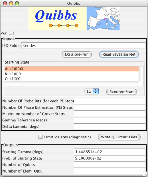
Figure 1: Control Panel of Quibbs

The Control Panel allows you to enter the following inputs:

I/O Folder:

Enter in this text box the name of a folder. The folder will contain Quibbs’ input and output files for the particular Bayesian network that you are currently considering. The I/O folder must be in the same directory as the Quibbs application.

To generate a quantum circuit, the I/O folder must contain the following 3 input files:

• parents.txt

• states.txt

• probs.txt

A detailed description of these 3 input files will be given in the next section. For this section, all you need to know is that: The parents.txt file lists the parent nodes of each node of the Bayesian net being considered. The states.txt file lists the names of the states of each node of the Bayesian net. And the probs.txt file gives the probability matrix for each node of the Bayesian net. Together, the In1, In2 and In3 files fully specify the Bayesian network being considered.

In Fig.1, “3nodes” is entered in the I/O Folder text box. A folder called “3nodes” comes with the distribution of Quibbs. It contains, among other things, In1, In2, In3 files that specify one possible Bayesian network with 3 nodes. The Quibbs distribution also comes with 3 other examples of I/O folders. These are named “2nodes”, “4nodeFullyConnected” and “Asia”.

When you press the Read Bayesian Net button, Quibbs reads files In1, In2 and In3. The program then creates data structures that contain complete information about the Bayesian network. Furthermore, Quibbs fills the scrollable list in the Starting State grouping with information that specifies “the starting state”. The starting state is one particular instantiation (i.e., a particular state for each node) of the Bayesian network. Each row of the scrollable list names a different node, and a particular state of that node. For example, Fig.1 shows the Quibbs Control Panel immediately after pressing the Read Bayesian Net button. In this example, the Bayesian net read in has 3 nodes called $A,B$ and $C$, and the starting state has node $A$ in state $a1$, node $B$ in state $b1$ and node $C$ in state $c1$.

Suppose $A$ is a node of the Bayesian net being considered. And suppose $A$ has $N_{A}$ states. Quibbs will give each state of node $A$ a “decimal name”; that is, a number from 0 through $N_{A}-1$. The “binary name” of a state is the binary representation of its decimal name. As shown in Fig.1, the scrollable list of the Control Panel gives not only the “english name” of the state of each node, but also the binary and decimal names of that state. For example, Fig.1 informs us that state $a1$ of node $A$ has binary name $(00)$ and decimal name $0$.

If you press the Random Start button, the starting state inside the scrollable list is changed to a randomly generated one. Alternative, you can choose a specific state for each node of the Bayesian net by using the Node State Menu, the menu immediately to the left of the Random Start button. To use the Node State Menu, you select the particular row of the scrollable list that you want to change. The Node State Menu mutates to reflect your row selection in the scrollable list. You can choose from the menu a particular node state. When you do so, the selected row in the scrollable list changes to reflect your menu choice.

When you press the Do a Pre-run button, Quibbs both reads and writes files: it reads files In1 and In2 (but not In3, so if In3 is not included in the I/O folder, this button still works), and it writes the following files, whose content will be described later:

• probsF.txt

• probsT.txt

• blankets.txt

• nits.txt

Number of Probe Bits (for each PE step):

This is the parameter $a=1,2,3,\ldots$ for the operator $V$.

Number of Phase Estimation (PE) Steps:

This is the parameter $c=1,2,3,\ldots$ for the operator $V$.

Maximum Number of Grover Steps:

Quibbs will stop iterating the AFGA if it reaches this number of iterations.

Gamma Tolerance (degs):

This is an angle given in degrees. Quibbs will stop iterating the AFGA if the absolute value of $\gamma_{j}$ becomes smaller than this tolerance. ($\gamma_{j}$ is an angle in AFGA that tends to zero as the iteration index $j$ tends to infinity. $\gamma_{j}$ quantifies how close the AFGA is to reaching the target state).

Delta Lambda (degs):

This is the angle $\Delta\lambda$ of AFGA, given in degrees.

Once Quibbs has successfully read files In1, In2 and In3, and once you have filled all the text boxes in the Inputs grouping, you can successfully press the Write Q. Circuit Files button. This will cause Quibbs to write the following output files within the I/O folder:

• quibbs_log.txt

• quibbs_eng.txt

• quibbs_pic.txt

The contents of these 3 output files will be described in detail in the next section. For this section, all you need to know is that: The quibbs_log.txt file records all the input and output parameters that you entered into the Control Panel, so you won’t forget them. The quibbs_eng.txt file is an in“english” description of a quantum circuit. And the quibbs_pic.txt file translates, line for line, the english description found in quibbs_eng.txt into a “pictorial” description.

Normally, you want to press the Write Q. Circuit Files button without check-marking the Omit V Gates (diagnostic) check box. If you do check-mark it, you will still generate files Out1,Out2, Out3, except that those files will omit to mention all those gates that generate the operator $V$, at every place were it would normally appear. Viewing the circuit without its $V$’s is useful for diagnostic and educational purposes, but such a circuit is of course useless for Gibbs sampling the Bayesian net being considered.

The Control Panel displays the following output text boxes. (The Starting Gamma (degs) output text box and the Prob. of Starting State output text box are both filled as soon as a starting state is given in the inputs. The other output text boxes are filled when you press the Write Q. Circuit Files button.)

Starting Gamma (degs):

This is $\gamma_{0}$, the first $\gamma_{j}$ in AFGA, given in degrees. In the notations of Ref.[6], and [8],

$$\gamma_{0} = {\rm acos}(\hat{s^{\prime}}\cdot\hat{t})=2\;{\rm acos}(|\langle s^{\prime}|t\rangle|)$$ (1a)

$$= 2\;{\rm acos}(\sqrt{P(x_{0})})\;,$$ (1b)

where $P(x_{0})$ is the Prob. of Starting State defined next.

Prob. of Starting State:

This is the probability $P(x_{0})$ in Ref.[6], where $P()$ is the full probability distribution of the Bayesian net ${\underline{x}}$ being considered, and $x_{0}$ is the starting value for ${\underline{x}}$.

Number of Qubits:

This is the total number of qubits used by the quantum circuit, equal to $2{N_{B}}+ac$ in the notation of Ref.[6].

Number of Elementary Operations:

This is the number of elementary operations in the output quantum circuit. If there are no LOOPs, this is the number of lines in the English File (see Sec. 4.2), which equals the number of lines in the Picture File (see Sec. 4.3). For a LOOP (assuming it is not nested inside a larger LOOP), the “LOOP k REPS:$N$” and “NEXT k” lines are not counted, whereas the lines between “LOOP k REPS:$N$” and “NEXT k” are counted $N$ times (because REPS:$N$ indicates $N$ repetitions of the loop body). Multiplexors expressed as a single line are counted as a single elementary operation (unless, of course, they are inside a LOOP, in which case they are counted as many times as the loop body is repeated).

3 Input Files

As explained earlier, for Quibbs to generate quantum circuit files, it needs to first read 3 input files: the Parents File called parents.txt, the States File called states.txt, and the Probabilities File called probs.txt. These 3 input files must be placed inside the I/O folder. Next we explain the contents of each of these 3 input files.

3.1 Parents File

Figure 2: Parents file in the I/O folder “3nodes”, for a Bayesian net with graph $A\rightarrow B\leftarrow C$

Fig.2 shows the Parents File as found in the folder “3nodes” which is included with the Quibbs distribution, for a Bayesian net with graph $A\rightarrow B\leftarrow C$. In this example, nodes $A$ and $C$ have no parents and node $B$ has parents $A$ and $C$.

In general, a Parents File must obey the following rules:

• Call focus nodes the node names immediately after a hash. Focus nodes in the States, Parents and Probabilities Files must all be in the same order. For example, in the “3nodes” case, that order is $A,B,C$.

• For each focus node, give a hash, then the name of the focus node, then a list of parents of the focus node, separating all of these with whitespace.

3.2 States File

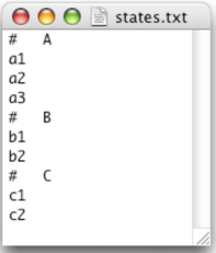
Figure 3: States file in the I/O folder “3nodes”, for a Bayesian net with graph $A\rightarrow B\leftarrow C$

Fig. 3 shows the States File as found in the folder “3nodes” which is included with the Quibbs distribution, for a Bayesian net with graph $A\rightarrow B\leftarrow C$. In this example, node $A$ has 3 states called $a1,a2$ and $a3$, node $B$ has 2 states called $b1$ and $b2$, and node $C$ has 2 states called $c1$ and $c2$.

In general, a States File must obey the following rules:

• Call focus nodes the node names immediately after a hash. Focus nodes in the States, Parents and Probabilities Files must all be in the same order. For example, in the “3nodes” case, that order is $A,B,C$.

• For each focus node, give a hash, then the name of the focus node, then a list of names of the states of the focus node, separating all of these with whitespace.

3.3 Probabilities File

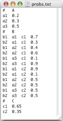
Figure 4: Probabilities File in the I/O folder “3nodes”, for a Bayesian net with graph $A\rightarrow B\leftarrow C$

Fig.4 shows the Probabilities File as found in the folder “3nodes” which is included with the Quibbs distribution, for a Bayesian net with graph $A\rightarrow B\leftarrow C$. In this example, $P_{A}(a1)=0.2$, $P_{B|A,C}(b1|a1,c1)=0.7$, etc.

In general, a Probabilities File must obey the following rules:

• Call focus nodes the node names immediately after a hash. Focus nodes in the States, Parents and Probabilities Files must all be in the same order. For example, in the “3nodes” case, that order is $A,B,C$.

• For each focus node, give a hash, then the name of the focus node, then the state of the focus node, then the states of each parent of the focus node, then the conditional probability of the focus node conditioned on its parents, separating all of these with whitespace.

• The order in which the states of the parents of the focus node are listed must be identical to the order in which the parents of that focus node are listed in the Parents File. For example, in the “3nodes” case, the Parents File gives the parents of node $B$ as $A,C$, in that order. Hence, in the Probabilities File, each conditional probability for focus node $B$ is given after giving the states of nodes $B,A,C$, in that order.

• A combination of node states may be omitted, in which case Quibbs will interpret that probability to be zero. For example, in “3nodes” case, if

  $$P_{B|A,C}(b1|a2,c2)=0,$$

  you could omit a line of the form

                 b1    a2    c2   0.0
  

  for the focus node $B$.

Note that Quibbs can help you to write a Probabilities File, by generating a template that you can change according to your needs. Such templates can be generated by means of the Do a Pre-run button. See Sec.4.4 for a detailed explanation of this.

4 Output Files

As explained earlier, when you press the Write Q. Circuit Files button, Quibbs writes 3 output files within the I/O folder: a Log File called quibbs_log.txt, an English File called quibbs_eng.txt, and a Picture File called quibbs_pic.txt. Next we explain the contents of each of these 3 output files. We also explain the contents of the various files generated when you press the Do a Pre-run button.

4.1 Log File

Figure 5: Log File generated by Quibbs using input files from the “3nodes” I/O folder.

Fig.5 is an example a Log File. This example was generated by Quibbs using the input files from the “3nodes” I/O folder. A Log File records all the information found in the Control Panel.

4.2 English File

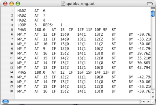
Figure 6: English File generated by Quibbs (with the Omit V Gates feature OFF) in the same run as the Log File of Fig.5, and using the input files from the “3nodes” I/O folder. Bottom of file is not visible. Right hand side of file is not visible.

Figure 7: English File generated by Quibbs (with the Omit V Gates feature ON) in the same run as the Log File of Fig.5, and using the input files from the “3nodes” I/O folder. Bottom of file is visible. Right hand side of file is visible.

Fig.6 (respectively, Fig.7) is an example of an English File. This example was generated by Quibbs, with the Omit V Gates feature OFF (respectively, ON), in the same run as the Log File of Fig.5, and using the input files from the “3nodes” I/O folder. An English File completely specifies the output SEO. It does so “in English”, thus its name. Each line represents one elementary operation, and time increases as we move downwards.

In general, an English File obeys the following rules:

• Time grows as we move down the file.

• Each row corresponds to one elementary operation. Each row starts with 4 letters that indicate the type of elementary operation.

• For a one-bit operation acting on a “target bit” $\alpha$, the target bit $\alpha$ is given after the word AT.

• If the one-bit operation is controlled, then the controls are indicated after the word IF. T and F stand for true and false, respectively. $\alpha$T stands for a control $P_{1}(\alpha)=n(\alpha)$ at bit $\alpha$. $\alpha$F stands for a control $P_{0}(\alpha)={\overline{n}}(\alpha)$ at bit $\alpha$.

• “LOOP k REPS:$N$” and “NEXT k” mark the beginning and end of $N$ repetitions. k labels the loop. k also equals the line-count number in the English file (first line is 0) of the line “LOOP k REPS:$N$”.

• SWAP $\alpha$ $\beta$ stands for the swap(i.e., exchange) operator $E(\alpha,\beta)$ that swaps bits $\alpha$ and $\beta$.

• PHAS $\theta^{degs}$ stands for a phase factor $e^{i\theta^{degs}\frac{\pi}{180}}$.

• P0PH $\theta^{degs}$ stands for the one-bit gate $e^{iP_{0}\theta^{degs}\frac{\pi}{180}}$ (note $P_{0}={\overline{n}}$). P1PH $\theta^{degs}$ stands for the one-bit gate $e^{iP_{1}\theta^{degs}\frac{\pi}{180}}$ (note $P_{1}=n$). Target bit follows the word AT.

• SIGX, SIGY, SIGZ, HAD2 stand for the Pauli matrices ${\sigma_{X}},{\sigma_{Y}},{\sigma_{Z}}$ and the one-bit Hadamard matrix $H$, respectively. Target bit follows the word AT.

• ROTX, ROTY, ROTZ, ROTN stand for one-bit rotations with rotation axes in the directions: $x$, $y$, $z$, and an arbitrary direction $n$, respectively. Rotation angles (in degrees) follow the words ROTX, ROTY, ROTZ, ROTN. Target bit follows the word AT.

• MP_Y stands for a multiplexor which performs a one-bit rotation of a target bit about the $y$ axis. Target bit follows the word AT. Rotation angles (in degrees) follow the word BY. Multiplexor controls are specified by $\alpha(k$, where integer $\alpha$ is the bit position and integer $k$ is the control’s name.

Here is a list of examples showing how to translate the mathematical notation used in Ref.[9] into the English File language:

Mathematical language	English File language
Loop named 5 with 2 repetitions	LOOP 5 REPS: 2
Next iteration of loop named 5	NEXT 5
$E(1,0)^{{\overline{n}}(3)n(2)}$	SWAP 1 0 IF 3F 2T
$e^{i42.7\frac{\pi}{180}{\overline{n}}(3)n(2)}$	PHAS 42.7 IF 3F 2T
$e^{i42.7\frac{\pi}{180}{\overline{n}}(3)n(2)}$	P0PH 42.7 AT 3 IF 2T
$e^{i42.7\frac{\pi}{180}n(3)n(2)}$	P1PH 42.7 AT 3 IF 2T
${\sigma_{X}}(1)^{{\overline{n}}(3)n(2)}$	SIGX AT 1 IF 3F 2T
${\sigma_{Y}}(1)^{{\overline{n}}(3)n(2)}$	SIGY AT 1 IF 3F 2T
${\sigma_{Z}}(1)^{{\overline{n}}(3)n(2)}$	SIGZ AT 1 IF 3F 2T
$H(1)^{{\overline{n}}(3)n(2)}$	HAD2 AT 1 IF 3F 2T
$(e^{i\frac{\pi}{180}23.7{\sigma_{X}}(1)})^{{\overline{n}}(3)n(2)}$	ROTX 23.7 AT 1 IF 3F 2T
$(e^{i\frac{\pi}{180}23.7{\sigma_{Y}}(1)})^{{\overline{n}}(3)n(2)}$	ROTY 23.7 AT 1 IF 3F 2T
$(e^{i\frac{\pi}{180}23.7{\sigma_{Z}}(1)})^{{\overline{n}}(3)n(2)}$	ROTZ 23.7 AT 1 IF 3F 2T
$(e^{i\frac{\pi}{180}[30{\sigma_{X}}(1)+40{\sigma_{Y}}(1)+11{\sigma_{Z}}(1)]})^{{\overline{n}}(3)n(2)}$	ROTN 30.0 40.0 11.0 AT 1 IF 3F 2T
$[e^{i\sum_{b1,b0}\theta_{b_{1}b_{0}}{\sigma_{Y}}(3)P_{b_{1}b_{0}}(2,1)}]^{n(0)}$	MP_Y AT 3 IF 2(1 1(0 0T BY 30.0 10.5 11.0 83.1
where $\left\{\begin{array}[]{l}\theta_{00}=30.0(\frac{\pi}{180})\\ \theta_{01}=10.5(\frac{\pi}{180})\\ \theta_{10}=11.0(\frac{\pi}{180})\\ \theta_{11}=83.1(\frac{\pi}{180})\end{array}\right.$

4.3 ASCII Picture File

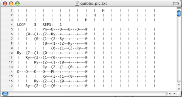
Figure 8: Picture File generated by Quibbs (with the Omit V Gates feature OFF) in the same run as the Log File of Fig.5, and using input files from the “3nodes” I/O folder. Bottom of file is not visible.

Figure 9: Picture File generated by Quibbs (with the Omit V Gates feature ON) in the same run as the Log File of Fig.5, and using input files from the “3nodes” I/O folder. Bottom of file is visible.

Fig.8 (respectively, Fig.9) is an example of a Picture File. This example was generated by Quibbs, with the Omit V Gates feature OFF (respectively, ON), in the same run as the Log File of Fig.5, and using the input files from the “3nodes” I/O folder. A Picture File partially specifies the output SEO. It gives an ASCII picture of the quantum circuit. Each line represents one elementary operation, and time increases as we move downwards. There is a one-to-one onto correspondence between the rows of the English and Picture Files.

In general, a Picture File obeys the following rules:

• Time grows as we move down the file.

• Each row corresponds to one elementary operation. Columns $1,5,9,13,\ldots$ represent qubits (or, qubit positions). We define the rightmost qubit as 0. The qubit immediately to the left of the rightmost qubit is 1, etc. For a one-bit operator acting on a “target bit” $\alpha$, one places a symbol of the operator at bit position $\alpha$.

• | represents a “qubit wordline” connecting the same qubit at two consecutive times.

• -represents a wire connecting different qubits at the same time.

• + represents both | and -.

• If the one-bit operation is controlled, then the controls are indicated as follows. @ at bit position $\alpha$ stands for a control $n(\alpha)=P_{1}(\alpha)$. 0 at bit position $\alpha$ stands for a control ${\overline{n}}(\alpha)=P_{0}(\alpha)$.

• “LOOP k REPS:$N$” and “NEXT k” mark the beginning and end of $N$ repetitions. k labels the loop. k also equals the line-count number in the Picture File (first line is 0) of the line “LOOP k REPS:$N$” .

• The swap(i.e., exchange) operator $E(\alpha,\beta)$ is represented by putting arrow heads < and > at bit positions $\alpha$ and $\beta$.

• A phase factor $e^{i\theta}$ for $\theta\in{\mathbb{R}}$ is represented by placing Ph at any bit position which does not already hold a control.

• The one-bit gate $e^{iP_{0}(\alpha)\theta}$ (note $P_{0}(\alpha)={\overline{n}}(\alpha)$) for $\theta\in{\mathbb{R}}$ is represented by putting OP at bit position $\alpha$.

• The one-bit gate $e^{iP_{1}(\alpha)\theta}$ (note $P_{1}(\alpha)=n(\alpha)$) for $\theta\in{\mathbb{R}}$ is represented by putting @P at bit position $\alpha$.

• One-bit operations ${\sigma_{X}}(\alpha)$, ${\sigma_{Y}}(\alpha)$, ${\sigma_{Z}}(\alpha)$ and $H(\alpha)$ are represented by placing the letters X,Y,Z, H, respectively, at bit position $\alpha$.

• One-bit rotations acting on bit $\alpha$, in the $x,y,z,n$ directions, are represented by placing Rx,Ry,Rz, R, respectively, at bit position $\alpha$.

• A multiplexor that rotates a bit $\tau$ about the $y$ axis is represented by placing Ry at bit position $\tau$. A multiplexor control at bit position $\alpha$ and named by the integer $k$ is represented by placing $(k$ at bit position $\alpha$.

Here is a list of examples showing how to translate the mathematical notation used in Ref.[9] into the Picture File language:

Mathematical language	Picture File language
Loop named 5 with 2 repetitions	LOOP 5 REPS:2
Next iteration of loop named 5	NEXT 5
$E(1,0)^{{\overline{n}}(3)n(2)}$	0---@---<--->
$e^{i42.7\frac{\pi}{180}{\overline{n}}(3)n(2)}$	0---@---+--Ph
$e^{i42.7\frac{\pi}{180}{\overline{n}}(3)n(2)}$	0P--@   |   |
$e^{i42.7\frac{\pi}{180}n(3)n(2)}$	@P--@   |   |
${\sigma_{X}}(1)^{{\overline{n}}(3)n(2)}$	0---@---X   |
${\sigma_{Y}}(1)^{{\overline{n}}(3)n(2)}$	0---@---Y   |
${\sigma_{Z}}(1)^{{\overline{n}}(3)n(2)}$	0---@---Z   |
$H(1)^{{\overline{n}}(3)n(2)}$	0---@---H   |
$(e^{i\frac{\pi}{180}23.7{\sigma_{X}}(1)})^{{\overline{n}}(3)n(2)}$	0---@---Rx  |
$(e^{i\frac{\pi}{180}23.7{\sigma_{Y}}(1)})^{{\overline{n}}(3)n(2)}$	0---@---Ry  |
$(e^{i\frac{\pi}{180}23.7{\sigma_{Z}}(1)})^{{\overline{n}}(3)n(2)}$	0---@---Rz  |
$(e^{i\frac{\pi}{180}[30{\sigma_{X}}(1)+40{\sigma_{Y}}(1)+11{\sigma_{Z}}(1)]})^{{\overline{n}}(3)n(2)}$	0---@---R   |
$[e^{i\sum_{b1,b0}\theta_{b_{1}b_{0}}{\sigma_{Y}}(3)P_{b_{1}b_{0}}(2,1)}]^{n(0)}$	|   Ry--(1--(0--@
where $\left\{\begin{array}[]{l}\theta_{00}=30.0(\frac{\pi}{180})\\ \theta_{01}=10.5(\frac{\pi}{180})\\ \theta_{10}=11.0(\frac{\pi}{180})\\ \theta_{11}=83.1(\frac{\pi}{180})\end{array}\right.$

4.4 Output Files From a Pre-run

When you press the Do a Pre-run button, Quibbs writes 4 output files within the I/O folder: two Uniform Probabilities Files called probsF.txt and probsT.txt, a Blankets File called blankets.txt, and a Nits File called nits.txt. Next we explain the contents of each of these 4 output files.

4.4.1 Uniform Probabilities Files

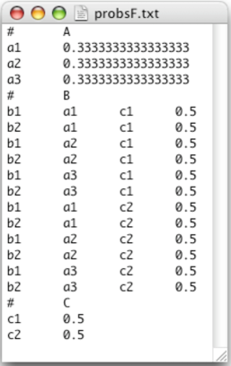
Figure 10: Uniform Probabilities File (of type probsF.txt) generated using input files from the “3nodes” I/O folder.

Figure 11: Uniform Probabilities File (of type probsT.txt) generated using input files from the “3nodes” I/O folder.

Figs.10 and 11 are both examples of a Uniform Probabilities File. Both files were generated by Quibbs using the input files from the “3nodes” I/O folder. A Uniform Probabilities File is simply a Probability File, as defined in Sec.3.3, but of a specific kind that assigns uniform values to all conditional probabilities of the Bayesian net specified by the Parents File and States File in the I/O Folder. Generating a Uniform Probabilities File (either probsF.txt or probsT.txt) does not require a probs.txt file. One can use a Uniform Probabilities File as a template for a probs.txt file. Just cut and paste the contents of a Uniform Probabilities File into a new file called probs.txt and modify its probabilities according to your needs. Note that the only difference between a probsF.txt and a probsT.txt file is that the first (respectively, second) of these varies the states of a focus node before (respectively, after) varying the states of its parents.

4.4.2 Blankets File

Figure 12: Blankets File generated using input files from the “3nodes” I/O folder.

Fig.12 is an example of a Blankets File. This example was generated by Quibbs using the input files from the “3nodes” I/O folder.

The Markov blanket $MB(i)$ for a node ${\underline{x}}_{i}$ of the classical Bayesian network ${\underline{x}}$ is defined so that (see section entitled “Notation and Preliminaries” in Ref.[10])

$$P(x_{i}|x_{\{i\}^{c}})=P(x_{i}|x_{MB(i)})\;.$$ (2)

It can be shown that the Markov blanket of a focus node equals the union of:

• the parents of the focus node

• the children of the focus node

• the parents of each children of the focus node (but excluding the focus node itself)

A Blankets File gives the Markov blanket for each node of a Bayesian net. In the example of Fig.12, node $A$ has Markov blanket $\{B,C\}$, etc.

In general, a Blankets File obeys the following rules:

• Call focus nodes the node names immediately after a hash.

• For each focus node, Quibbs writes a hash, then the name of the focus node, then a list of the nodes which form the Markov blanket of the focus node.

4.4.3 Nits File

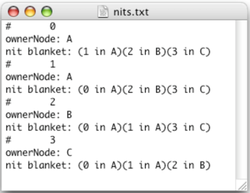
Figure 13: Nits File generated using input files from the “3nodes” I/O folder.

Fig.13 is an example of a Nits File. This example was generated by Quibbs using the input files from the “3nodes” I/O folder.

The word “nit” is a contraction of the words “node” and “qubit”. Quibbs assigns to each node (of the Bayesian net being consider) its own private set of nits. We explained in Sec.2 how Quibbs assigns a decimal and a binary name to each state of a node. The binary name of a state gives the states of the nits. For example, suppose node $A$ has 3 states: $a1(00)0$, $a1(01)1$ and $a1(10)2$. Then node $A$ is assigned two private nits, call them $nit0$ and $nit1$. When node $A$ is in state $(b1,b0)$, where $b1$ and $b0$ are either 0 or 1, then $nit1$ is in state $b1$ and $nit0$ is in state $b0$.

Actually, Quibbs doesn’t give nits an “english” name like $nit0$ and $nit1$. It just calls them by integers. Fig.13 informs us that the “3nodes” Bayesian net has 4 nits called 0,1,2,3. Nits 0 and 1 are both owned by node $A$ (which has 3 states $a1,a2,a3$). Nit 2 is owned by node $B$ (which has 2 states $b1,b2$). Nit 3 is owned by node $C$ (which has 2 states $c1,c2$).

The original Bayesian net with the original nodes implies a new, finer Bayesian net whose nodes are the nits themselves. Just like one can define a Markov blanket for each node of the original Bayesian net, one can define a Markov blanket ( equal to a particular set of nits) for each nit. Fig.13 informs us that for the “3nodes” Bayesian net, nit 0 has a nit blanket $\{1,2,3\}$, etc.

In general, a Nits File obeys the following rules:

• Call focus nit the number ( a sort of nit name) immediately after a hash.

• For each focus nit, Quibbs writes the words “owner node” followed by the name of the owner node of the focus nit.

• For each focus nit, Quibbs writes the words “blanket nit” followed by the Markov blanket of nits for the focus nit.

Why do we care about node blankets and nit blankets at all? Quibbs uses a method, discussed in Ref.[6], of representing Szegedy operators using quantum multiplexors. Quibbs uses nit blankets to simplify its Szegedy representations by eliminating certain unnecessary controls in their multiplexors.

References

- [1] R.R. Tucci, “A Rudimentary Quantum Compiler(2cnd Ed.)”, arXiv:quant-ph/9902062 . Qubiter software available at www.ar-tiste.com
- [2] R.R. Tucci, “QuanTree and QuanLin, Two Special Purpose Quantum Compilers”, arXiv:0712.3887
- [3] R.R. Tucci, “QuanFou, QuanGlue, QuanOracle and QuanShi, Four Special Purpose Quantum Compilers”, arXiv:0802.2367
- [4] R.R. Tucci, “Java Application that Outputs Quantum Circuit for Some NAND Formula Evaluators”, arXiv:0802.2370
- [5] R.R. Tucci, “Code Generator for Quantum Simulated Annealing”, arXiv:0908.1633
- [6] R.R. Tucci, “Quantum Gibbs Sampling Using Szegedy Operators”, arXiv:0910.1647
- [7] R.R. Tucci, “Use of Quantum Sampling to Calculate Mean Values of Observables and Partition Function of a Quantum System”, arXiv:0912.4402
- [8] R.R. Tucci, “An Adaptive, Fixed-Point Version of Grover’s Algorithm”, arXiv:1001.5200
- [9] R.R. Tucci, “How to Compile Some NAND Formula Evaluators”, arXiv:0706.0479
- [10] R.R. Tucci, “Use of a Quantum Computer to do Importance and Metropolis-Hastings Sampling of a Classical Bayesian Network”, arXiv:0811.1792