Abstract

For SU(3) lattice gauge theory we study properties of static quark sources represented by local Polyakov loops. We find that for temperatures both below and above $T_{c}$ coherent domains exist where the phases of the local loops have similar values in the vicinity of the center values $0,\pm 2\pi/3$. The cluster properties of these domains are studied numerically. We demonstrate that the deconfinement transition of SU(3) may be characterized by the percolation of suitably defined clusters.

To appear in Physics Letters B

Introductory remarks Confinement and the transition to a deconfining phase at high temperatures are important, but not yet sufficiently well understood properties of QCD. With the running and upcoming experiments at the RHIC, LHC and GSI facilities, it is important to also obtain a deeper theoretical understanding of the mechanisms that drive the various transitions in the QCD phase diagram.

An influential idea is the Svetitsky-Jaffe conjecture [1] which states that for pure gluodynamics the critical behavior can be described by an effective spin model in 3 dimensions which is invariant under the center group $\mathds{Z}_{3}$ (for gauge group SU(3)). The spin degrees of freedom are related [2] to static quark sources represented by Polyakov loops, which in a lattice regularization are given by

$$L(\vec{x})\,=\,\mbox{tr}_{c}\prod_{t=1}^{N}U_{4}(\vec{x},t)\;.$$ (1)

The Polyakov loop $L(\vec{x})$ is defined as the ordered product of the SU(3) valued temporal gauge variables $U_{4}(\vec{x},t)$ at a fixed spatial position $\vec{x}$, where $N$ is the number of lattice points in time direction and $\mbox{tr}_{c}$ is the trace over color indices. The loop $L(\vec{x})$ thus is a gauge transporter that closes around compactified time. Often also the spatially averaged loop $P=1/V\sum_{\vec{x}}L(\vec{x})$ is considered, where $V$ is the spatial volume. Due to translational invariance $P$ and $L(\vec{x})$ have the same vacuum expectation value.

The Polyakov loop corresponds to a static quark source and its vacuum expectation value is (after a suitable renormalization) related to the free energy $F_{q}$ of a single quark, $\langle P\rangle\propto\exp(-F_{q}/T)$, where $T$ is the temperature (the Boltzmann constant is set to 1 in our units). Below the critical temperature $T_{c}$ quarks are confined and $F_{q}$ is infinite, implying $\langle P\rangle=0$. This is evident in the lhs. plot of Fig. 1 where we show scatter plots of the values of the Polyakov loop $P$ in the complex plane for 100 configurations below (lhs. panel) and above $T_{c}$ (rhs.) . In the high temperature phase quarks become deconfined leading to a finite $F_{q}$ which gives rise to a non-vanishing Polyakov loop (rhs. in Fig. 1).

On a finite lattice, above $T_{c}$ the phase of the Polyakov loop assumes values near the center phases which for SU(3) are $0,\pm 2\pi/3$ (rhs. plot of Fig. 1). This is a reflection of the underlying center symmetry which is a symmetry of the action and the path integral measure of gluodynamics, that is broken spontaneously above the deconfinement temperature $T_{c}$. As long as the volume is finite all three sectors are populated, while in an infinite volume only one of the three phase values survives. This center symmetry and its spontaneous breaking are the basis for the above mentioned Svetitsky-Jaffe conjecture [1].

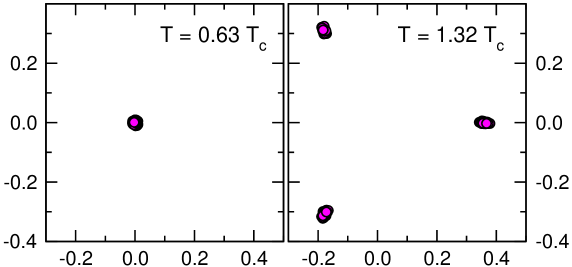
Figure 1: Scatter plots of the spatially averaged Polyakov loop $P$ in the complex plane for configurations below (lhs. panel) and above $T_{c}$ (rhs.). We show the results for our $40^{3}\times 6$ ensembles.

The relation of the deconfinement transition of SU($N$) gauge theory to $\mathds{Z}_{N}$-symmetric spin models has an interesting implication: For such spin models it is known that suitably defined clusters made from neighboring spins that point in the same direction show the onset of percolation at the same temperature where the $\mathds{Z}_{N}$-symmetry is broken spontaneously. For, e.g., the Ising system these percolating clusters were identified [6] as the Fortuin-Kasteleyn clusters [7]. An interesting question is whether the cluster- and percolation properties can be directly observed in a lattice simulation of gluodynamics – without the intermediate step of the effective spin theory [2] for the Polyakov loops.

For the case of gauge group SU(2) such cluster structures were analyzed in a series of papers [8, 9], while for SU(3) the formation of center clusters has not yet been explored. In this paper we try to close this gap and study the behavior of the local loops $L(\vec{x})$ and the possible formation of center clusters. Furthermore, we study center clusters not only near $T_{c}$ (where they directly can be expected from the Svetitsky-Yaffe conjecture) but explore their emergence and properties in a window of temperatures ranging from 0.63 $T_{c}$ to 1.32 $T_{c}$.

Properties of local Polyakov loops For analyzing spatial structures of $L(\vec{x})$ on individual configurations we write the local loops in terms of a modulus $\rho(\vec{x})$ and a phase $\varphi(\vec{x})$,

$$L(\vec{x})\;=\;\rho(\vec{x})\,e^{\,i\,\varphi(\vec{x})}\;.$$ (2)

The first step of our investigation is to study the behavior of the modulus $\rho(\vec{x})$. In Fig. 2 we show histograms for the distribution of $\rho(\vec{x})$ in the confined (lhs. plot) and the deconfined phase (rhs.). It is obvious, that the distributions of the modulus $\rho(\vec{x})$ below and above $T_{c}$ are almost indistinguishable. Furthermore we find that the distribution follows very closely the distribution according to Haar measure, which we show as a full curve. Only above $T_{c}$ we observe a very small deviation from the Haar measure distribution. The Haar measure distribution curves for the modulus and the phase are defined as

$$P(\rho)\;=\;\int D[U]\,\delta(\rho-|\,\mbox{Tr}\,[U]|)\;,\;P(\varphi)\;=\;\int D[U]\,\delta(\varphi-\mbox{arg Tr\, }[U])\;,$$ (3)

where $\delta$ is the Dirac delta-function and $D[U]$ is the Haar integration measure for group elements $U\in$ SU(3). These two distributions are obtained from a single group element and thus do not depend on any lattice parameters.

From the fact that the change of the modulus is very small we conclude that the jump of $\langle P\rangle$ at $T_{c}$, signaling the first order deconfinement transition, is not driven by a changing modulus of the local loops $L(\vec{x})$.

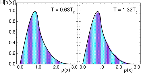
Figure 2: Histograms for the distribution of the modulus $\rho(\vec{x})$ of the local loops $L(\vec{x})$ for temperatures below and above $T_{c}$. The full curve is the distribution according to Haar measure ($40\times 6$ ensembles).

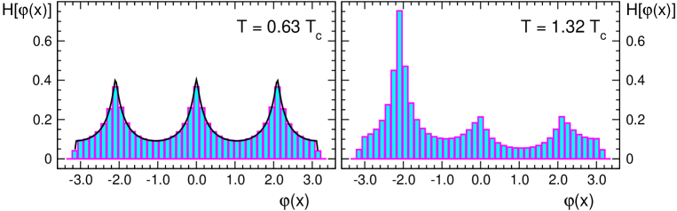
Figure 3: Histograms for the distribution of the phase $\varphi(\vec{x})$ of the local loops $L(\vec{x})$. We compare the distribution below $T_{c}$ (lhs. plot) to the distribution in the deconfined phase (rhs.) for the sector of configurations with phases of the averaged loop $P$ near $-2\pi/3$. The full curve in the lhs. plot is the distribution according to Haar measure ($40\times 6$ ensembles).

Thus we focus on the behavior of the phase $\varphi(\vec{x})$, and again study histograms for its distribution. In Fig. 3 we compare the distribution below $T_{c}$ (lhs. plot) to the one in the deconfined phase (rhs.). For the latter we show the distribution for the sector of configurations characterized by phases of the averaged Polyakov loop $P$ in the vicinity of $-2\pi/3$ (compare the rhs. of Fig. 1).

The distribution of the phases $\varphi(\vec{x})$ is rather interesting: Also in the confined low temperature phase (lhs. plot in Fig. 3) the distribution clearly is peaked at the center phases $-2\pi/3$, $0$ and $+2\pi/3$, and again perfectly follows the Haar measure distribution (full curve in the lhs. plot). The distribution is identical around these three phases and the vanishing result for $\langle P\rangle$ below $T_{c}$ comes from a phase average, $1+e^{i2\pi/3}+e^{-i2\pi/3}=0$.

Above $T_{c}$ (rhs. plot in Fig. 3) the distribution singles out one of the phases. In our case, where configurations in the sector with phases of the averaged loop $P$ near $-2\pi/3$ are used for the plot, it is the value $-2\pi/3$ which is singled out. For configurations in one of the other two sectors (see rhs. plot of Fig. 1) the distribution is shifted periodically by $\pm 2\pi/3$. Obviously, above $T_{c}$ the distribution is not equal for the three center phases and the cancellation of phases does no longer work, resulting in a non-zero $\langle P\rangle$.

The histograms for the phases $\varphi(\vec{x})$ suggest that at the critical temperature the local loops $L(\vec{x})$ start to favor phases near one spontaneously selected center value, while phases near the other two center values are depleted. This is illustrated in more detail in Fig. 4 where we show the abundance $A$ of lattice points with phases of $L(\vec{x})$ near the dominant and subdominant center values. To define the abundance $A$ we cut the interval $(-\pi,\pi)$ at the minima of the distribution of Fig. 3 into the three sub-intervals $(-\pi,-\pi/3)$, $(-\pi/3,\pi/3)$, $(\pi/3,\pi)$, which we refer to as “center sectors”. We count the number of lattice points with phases in each of the three center sectors and obtain their abundance $A$ by normalizing these counts with the volume. Fig. 4 shows that at low temperatures all three center sectors are populated with probability 1/3. Near $T_{c}$ one of the sectors starts to dominate while the other sectors are depleted.

Coherent center domains We have demonstrated for a wide range of temperatures that the center sectors play an important role for the phases $\varphi(\vec{x})$ of the local loops $L(\vec{x})$, which cluster near the center phases $0,\pm 2\pi/3$ at all temperatures. The deconfinement transition is manifest in the onset of a dominance of one spontaneously selected center sector. We now analyze whether the values of the phases $\varphi(\vec{x})$ are distributed homogeneously in space, or if instead there exist spatial domains with coherent phase values in the same sector.

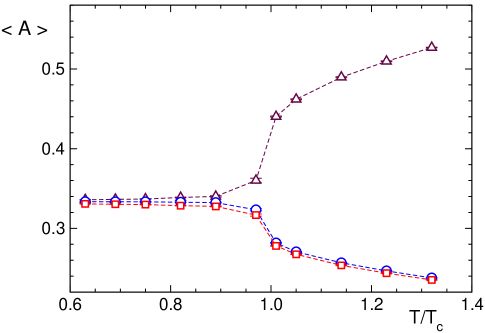
Figure 4: Abundance of lattice points $\vec{x}$ with phases of the local loop $L(\vec{x})$ in the dominant (triangles) and subdominant center sectors (circles, squares) as a function of temperature ($40\times 6$ ensembles).

In order to study such domains, we use sub-intervals that divide the interval $(-\pi,\pi)$ for the values of the $\varphi(\vec{x})$. For a more general analysis we introduce the cutting parameter $\delta\geq 0$ and define the three sub-intervals as $(-\pi+\delta,-\pi/3-\delta)$, $(-\pi/3+\delta,\pi/3-\delta)$ and $(\pi/3+\delta,\pi-\delta)$ (which we again refer to as “center sectors”). For $\delta=0$ we obtain the old sub-intervals, while a value of $\delta>0$ allows us to cut out lattice points where the phases are near the minima of the distributions shown in Fig. 3.

The definition of the clusters slightly differs from those that have been used for the analysis [8, 9] of clusters in SU(2) gauge theory. Besides modifications of the Fortuin-Kasteleyn prescription studied in [8], in [9] the bonding probability between neighboring sites with same sign Polyakov loops was introduced as a free parameter. This parameter could then be tuned such that the onset of percolation agrees with the deconfinement temperature. In our definition the parameter $\delta$ allows one to reduce the lattice to a skeleton of points with phases close to the center elements (in intervals of width $2(\pi/3-\delta)$ around the center values). For the plots shown in Figs. 5 and 6 we choose $\delta$ such that roughly those 40 % of lattice points are cut where the phases do not strongly lean towards one of the center values. We found that near $T_{c}$ the critical properties of the clusters (behavior of largest cluster and percolation) are stable when $\delta$ is varied in a small interval around that value [11] (compare also the discussion in [9]). For example the curve for the weight of the largest cluster (see Fig. 5 below, where we show a comparison of different spatial volumes for a cut of 39 %) is form-invariant in a range of cuts from 30 % to 45 % and only is rescaled by a change of the amplitude of less than 15 %.

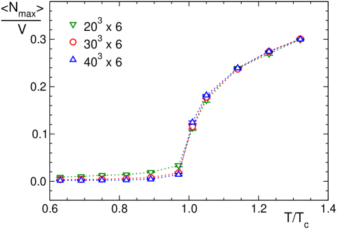
Figure 5: Weight of the largest center cluster as a function of temperature.

In a next step we define clusters by assigning neighboring lattice sites with phases $\varphi(\vec{x})$ in the same center sector to the same cluster. Once these center clusters are defined we can study their properties and behavior with temperature using concepts developed for the percolation problem [10]. In Fig. 5 we show the weight (i.e., the number of sites) of the largest cluster as a function of the temperature. For low temperatures all clusters are small, while as $T$ is increased towards the deconfinement temperature the largest cluster starts to grow quickly and above $T_{c}$ scales with the volume. This property indicates that in the deconfined phase the system has developed a percolating cluster. The onset of percolation at $T_{c}$ is confirmed in Fig. 6 where we show the percolation probability $p_{\infty}$ as a function of $T/T_{c}$. The percolation probability is computed by averaging an observable which is 1 if a spanning cluster exists and 0 otherwise. In our case, where we have periodic spatial boundary conditions, a spanning cluster is defined as a cluster who has at least one member site in every $y$-$z$ plane. In other words, we analyze percolation in $x$ direction, which is, however, no loss of generality as we have invariance under discrete spatial rotations. Varying $\delta$ in a range where the number of points we cut varies between 30 and 45 % (Fig. 6 is for 39 %), slightly roundens the transition curve, but leaves the onset of percolation unchanged at $T/T_{c}=1$.

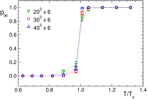
Figure 6: Percolation probability $p_{\infty}$ of the dominant center clusters as a function of temperature.

An interesting question is the size of the clusters in physical units in the confining phase, which could be related to some hadronic scale (see also the discussion in the next section). In order to study this cluster size below $T_{c}$ we computed 2-point correlation functions of points within the individual clusters. These correlators decay exponentially $\propto\exp(-r/\xi)$ with distance $r$, and the factor $\xi$ defines a linear size of the clusters in lattice units. We then analyze $d\equiv 2\,\xi\,a$, which gives a definition of the cluster diameter in physical units ($a$ is the lattice spacing in fm). We find that up to $T=0.85T_{c}$ this diameter is essentially independent of the temperature, with a value of $d=0.46(5)$ fm at a cut of 39 % and $d=0.62(7)$ fm at a cut of 30 %. Compared to the expected sizes of rougly 0.5 fm for heavy quark mesons this is a quite reasonable result for the linear scale of the clusters which suggests that the physical role of the clusters below $T_{c}$ should be studied in more detail (see [11]).

Summary and discussion We have explored the clustering of the phases $\varphi(\vec{x})$ of the local quark sources $L(\vec{x})$ near the center values, both below and above $T_{c}$. We find that in the range of temperatures we consider, $T=0.63\,T_{c}$ to $T=1.32\,T_{c}$, the local Polyakov loop phases prefer values near the center values and corresponding clusters may be identified for these temperatures. Using the parameter $\delta$ we can construct clusters such that the deconfinement transition is characterized by percolation of the clusters in the dominant sector.

From the cluster properties a simple qualitative picture for confinement and the deconfinement transition emerges. Below $T_{c}$ the clusters of lattice points which have the same center phase information are small. Only if a quark- and an anti-quark source are sufficiently close to each other they fit into the same cluster and can have a non-vanishing expectation value. Sources at distances larger than a typical cluster size receive the independent center fluctuations from different clusters and the correlator averages to zero. Above $T_{c}$ the clusters percolate and coherent center information is available also for larger distances allowing for non-vanishing correlation at large separation of the sources. In this picture deconfinement is a direct consequence of a percolating center cluster.

A possible role of local center structures for confinement has been addressed also in a different approach, using a projection of the link variables $U_{\mu}(\vec{x},t)$ at all points in space and time to a center element after fixing to a suitable gauge (see, e.g., [12] for a selection of recent results). This analysis is motivated by understanding the role of topological objects for the QCD phase transition. It would be highly interesting to study a possible connection of the percolation aspects of the transition to the dynamics of such topological objects. Of particular relavance would be an analysis of a possible relation to calorons which induce strong local variations of the Polyakov loop that might play an important role in the formation of the center clusters [13].

We conclude with a few comments on the extension of the center domain picture to the case of full QCD: The fermion determinant describing the dynamical quarks can be expressed as a sum over closed loops, which may be viewed as generalized Polyakov loops and are sensitive to the center properties of the gauge fields [14]. The fermion determinant breaks the center symmetry explicitly and acts like an external magnetic field which favors the real sector (phase 0) for the Polyakov loop $P$. However, preliminary numerical results with dynamical fermions [11] show that locally also the two complex sectors (phases $\pm 2\pi/3$) remain populated. The corresponding clusters will again lead to a coherent phase information for sufficiently close quark lines. As for the pure gauge theory studied in this letter, the preliminary results [11] show that the transition to confinement is again accompanied by a pronounced increase of the abundance for the dominant (i.e., real) sector. However, the explicit symmetry breaking through the determinant leads to a crossover type of behavior in the dynamical case. An interesting related question, which has already been raised in the literature [15], is whether also the chiral transition may be characterized as a percolation phenomenon.

Acknowledgments: The author thanks Mike Creutz, Julia Danzer, Mitja Diakonov, Christian Lang, Ludovit Liptak, Axel Maas, Stefan Olejnik, Alexander Schmidt and Andreas Wipf for valuable comments. The numerical calculations were done at the ZID clusters of the University Graz.

References

- [1] L.G. Yaffe, B. Svetitsky, Phys. Rev. D 26 (1982) 963; Nucl. Phys. B 210 (1982) 423.
- [2] J. Polonyi, K. Szlachanyi, Phys. Lett. B 110 (1982) 395; M. Ogilvie, Phys. Rev. Lett. 52 (1984) 1369; F. Green, F. Karsch, Nucl. Phys. B 238 (1984) 297; S. Fortunato, F. Karsch, P. Petreczky and H. Satz, Phys. Lett. B 502 (2001) 321; C. Wozar, T. Kaestner, A. Wipf, T. Heinzl, B. Pozsgay, Phys. Rev. D 74 (2006) 114501; A. Wipf, T. Kaestner, C. Wozar, T. Heinzl, SIGMA 3 (2007) 006; C. Wozar, T. Kaestner, A. Wipf, T. Heinzl, Phys. Rev. D 76 (2007) 085004.
- [3] M. Lüscher, P. Weisz, Commun. Math. Phys. 97 (1985) 59 [Err.: 98 (1985) 433]; G. Curci, P. Menotti, G. Paffuti, Phys. Lett. B 130 (1983) 205 [Err.: B 135 (1984) 516].
- [4] C. Gattringer, R. Hoffmann, S. Schaefer, Phys. Rev. D 65 (2002) 094503.
- [5] C. Gattringer, P.E.L. Rakow, A. Schäfer, W. Söldner, Phys. Rev. D 66 (2002) 054502.
- [6] A. Coniglio and W. Klein, J. Phys. A 13 (1980) 2775.
- [7] C.M. Fortuin and P. W. Kasteleyn, Physica 57 (1972) 536.
- [8] S. Fortunato, H. Satz, Phys. Lett. B 475 (2000) 311; S. Fortunato and H. Satz, Nucl. Phys. A 681 (2001) 466.
- [9] S. Fortunato, J. Phys. A 36 (2003) 4269.
- [10] G.R. Grimmett, Percolation, Springer, New York, 1999.
- [11] C. Gattringer et al, work in preparation.
- [12] R. Bertle, M. Faber, J. Greensite, S. Olejnik, JHEP 9903 (1999) 019; M. Engelhardt, K. Langfeld, H. Reinhardt, O. Tennert, Phys. Rev. D 61 (2000) 054504; J. Greensite, Prog. Part. Nucl. Phys. 51 (2003) 1; M. Engelhardt, Nucl. Phys. Proc. Suppl. 140 (2005) 92; M. Pepe, PoS LAT2005 (2006) 017; J. Greensite, K. Langfeld, S. Olejnik, H. Reinhardt, T. Tok, Phys. Rev. D 75 (2007) 034501; V.G. Bornyakov, E.M. Ilgenfritz, B.V. Martemyanov, S.M. Morozov, M. Müller-Preussker and A. I. Veselov, Phys. Rev. D 77 (2008) 074507.
- [13] E.M. Ilgenfritz, M. Müller-Preussker and D. Peschka, Phys. Rev. D 71 (2005) 116003; F. Bruckmann, E.M. Ilgenfritz, B. Martemyanov and B. Zhang, Phys. Rev. D 81 (2010) 074501.
- [14] C. Gattringer, L. Liptak, arXiv:0906.1088 [hep-lat].
- [15] M. Beccaria and A. Moro, Phys. Rev. D 66 (2002) 037502 [Erratum-ibid. D 72 (2005) 029901].