Non-perturbative Corrections to Particle Production from Coherent Oscillation

Abstract

We investigate particle production from coherent oscillation by using the method based on the Bogolyubov transformation. Especially, we study the case when the amplitude of the oscillation and also the coupling constants with the oscillating field are small in order to avoid the non-perturbative corrections from the broad parametric resonance. We derive the expressions for the distribution functions and the number densities of produced particles at the leading order of coupling constant. It is, however, found that these results fail to describe the exact particle production eventually due to the non-perturbative effects even if the coupling constants are small. We then introduce a simple method to handle with such corrections, i.e., the time averaging method. It is shown that this method successfully provides the evolution of the occupation numbers of the growing mode. Further, we point out that the approximate results by this method satisfy the exact scaling properties coming from the periodicity of the coherent oscillation.

1 Introduction

Coherent oscillation of scalar field plays an important role to describe various phenomena in particle physics and particle cosmology. One of the most important examples is the so-called slow-roll model of the inflationary universe. [1, 2] A scalar field, called as inflaton, is initially displaced from the potential minimum and its vacuum energy leads to the de-Sitter expansion of the universe. This class of models elegantly solves the flatness and horizon problems of the standard Big Bang cosmology. Moreover, it can give an origin of the density fluctuations which is strongly supported from the recent measurements of the cosmic microwave background radiation. [3] After the inflation ends, the inflaton starts to cause coherent oscillation around its potential minimum.

The energy of coherent oscillation is diluted due to the expansion of the universe as well as the energy transfer to particles though interaction of the oscillating field. Produced particles are then thermalized and the hot universe can be realized. The whole of these processes is called as the reheating. In particular, the reheating of the slow-roll inflation gives an initial condition of the standard Big Bang cosmology. Therefore, the reheating process is crucial for understanding the very early universe.

In this paper, we focus on the first stage of the reheating, i.e., particle production from coherent oscillation. This process has been widely discussed based on that coherent oscillation is considered as non-relativistic scalar particles, [4]  and particles are produced through their decay and/or scattering processes. [5]  In this case the number of parent non-relativistic particles is given by the energy of coherent oscillation divided by the mass of the oscillating field, and the number of produced particles is determined by it. On the other hand, it has been pointed out that, when the coupling with produced particles and also the amplitude of the oscillation become large, the non-perturbative effect becomes significant in the early stage of particle production [6, 7, 8, 9].  This process is called as the preheating. [7]  Especially, the explosive production of bosonic degrees of freedom can happen due to the broad parametric resonance effect. On the other hand, the fermion production at the preheating has been also investigated. [10, 11, 12]

The purpose of this paper is to investigate the production of scalars and fermions from coherent oscillation, especially when the coupling constants of oscillating field are very small to avoid the effect of the broad parametric resonance. For this purpose, we apply the method based on the Bogolyubov transformations. [13, 14] In this case, the equation of motion for the mode functions of produced particles in the presence of coherent oscillation is solved and the growth of the mode functions are then interpreted as the production of particles. First, we will present the analytical formulae for the distribution functions and the number densities of produced particles by using the perturbative expansion of the coupling constants. We will also discuss the conditions under which the perturbative results are justified. Indeed, it will be shown that the leading-order results collapse in the end.

This is a signal that the non-perturbative effect becomes important even if the coupling constant is sufficiently small. Such a correction is crucial for describing the statistical properties of produced particles, namely the effects of the Bose condensation for the scalar production and the Pauli blocking for the fermion production. In order to handle the annoying non-perturbative effects we will present the time averaging method, which is familiar in the nonlinear dynamical system. [15] It will be demonstrated that this method is powerful to extract the characteristic evolution of the occupation number for the growing mode, i.e., the exponential growth for scalar production or the oscillation between 0 to 1 for fermion production. Furthermore, we will show that the results by the time averaging method obey the exact scaling property, which is obtained from the periodicity of the the equation of motion. [16] This gives a justification for the use of the time averaging method. Throughout the present analysis we neglect the expansion of the universe for simplicity.

The rest of this paper is organized as follows. In Sec. 2 we explain the model in this analysis. We perform in Sec. 3 the perturbative estimation of the yields when the amplitude of the coherent oscillation is sufficiently small. The importance of non-perturbative effects in particle production is addressed in Sec. 4. We present the time averaging method to deal with such effects, and try to figure out the statistical properties of produced particles. Finally, the last section is devoted to conclusion. We also add Appendix A to explain the perturbative estimation of the number density.

2 Framework

To begin with, let us explain the framework of this analysis. We shall study the production of real scalar field $\chi$ and Dirac fermion $\psi$ from the coherently oscillating $\phi$ by using Lagrangian

$${\cal L} = \frac{1}{2}\,(\partial_{\mu}\phi)(\partial^{\mu}\phi)-V(\phi)+\frac{1}{2}\,(\partial_{\mu}\chi)(\partial^{\mu}\chi)-\frac{1}{2}\,g_{S}^{2}\,\phi^{2}\,\chi^{2}+i\,\overline{\psi}\gamma_{\mu}\partial^{\mu}\psi-g_{F}\,\phi\,\overline{\psi}\,\psi\,,$$ (1)

where $g_{S}$ and $g_{F}$ are coupling constants. For definiteness, we take here the potential for the real scalar field $\phi$ as

$$V(\phi)=\frac{1}{2}\,m_{\phi}^{2}\,\Bigl{(}\phi-\langle\phi\rangle\Bigr{)}^{2}\,,$$ (2)

where $m_{\phi}$ and ${\langle\phi\rangle}$ are mass and vacuum expectation value (vev) of $\phi$, respectively, and they are taken to be real and positive. At the potential minimum $\chi$ and $\psi$ receive masses as $m_{\chi}=g_{S}{\langle\phi\rangle}$ and $m_{\psi}=g_{F}{\langle\phi\rangle}$. From now on the field $\phi$ is assumed to oscillate coherently around ${\langle\phi\rangle}$ with an amplitude $\Phi$

$$\phi(t)={\langle\phi\rangle}+\Phi\,\cos(m_{\phi}t)\,,$$ (3)

and it is treated as a classical background field. Notice that we neglect the expansion of the universe throughout the present analysis.

Particle production from the $\phi$ oscillation is usually discussed as follows: The coherent oscillation is considered as non-relativistic particles [4]. In this case, the energy density of the $\phi$ oscillation is $\rho_{\phi}=\dot{\phi}{}^{2}/{2}+V(\phi)=m_{\phi}^{2}\,\Phi^{2}/2$ (here and hereafter the dot denotes a derivative with respect to time), and the number density of $\phi$ is estimated as $n_{\phi}=\rho_{\phi}/m_{\phi}=m_{\phi}\,\Phi^{2}/2$. Decays of $\phi$, $\phi\to\chi+\chi$ and $\phi\to\psi+\overline{\psi}$, are important processes to produce $\chi$ and $\psi$. The partial rates of these processes are found from Eq. (1) as

$$\Gamma_{\phi\to\chi+\chi} = \frac{g_{S}^{2}\,\beta_{\chi}}{8\pi}\,\frac{m_{\chi}^{2}}{m_{\phi}}\,,$$ (4)

$$\Gamma_{\phi\to\psi+\overline{\psi}} = \frac{g_{F}^{2}\,\beta_{\psi}^{3}}{8\pi}\,m_{\phi}\,,$$ (5)

where $\beta_{\chi,\psi}=\sqrt{1-4m_{\chi,\psi}^{2}/m_{\phi}^{2}}$. The number densities of $\chi$ and $\psi$ from the decays of $\phi$ are then estimated as

$$n_{\chi}(t) = 2\,\Gamma_{\phi\to\chi+\chi}\,n_{\phi}\,t=\frac{g_{S}^{2}\,\beta_{\chi}\,\Phi^{2}\,m_{\chi}^{2}}{8\pi}\,t\,,$$ (6)

$$n_{\psi}(t) = 2\,\Gamma_{\phi\to\psi+\overline{\psi}}\,n_{\phi}\,t=\frac{g_{F}^{2}\,\beta_{\psi}^{3}\,\Phi^{2}\,m_{\phi}^{2}}{8\pi}\,t\,.$$ (7)

It is seen that $n_{\chi,\psi}$ are proportional to $t$ by neglecting the decrease of $n_{\phi}$, and that they are induced at the order of coupling squared.

Further, the scattering processes of $\phi$’s are another sources of particle production. The number density of $\chi$ due to the process $\phi+\phi\to\chi+\chi$ is estimated as $n_{\chi}(t)=\langle\sigma v_{\phi}\rangle\,n_{\phi}^{2}\,t$, where $v_{\phi}$ is the relative velocity of $\phi$’s and $\langle\sigma v_{\phi}\rangle$ is the invariant scattering rate which is given by $\langle\sigma v_{\phi}\rangle=g_{S}^{4}\,\beta_{\chi}^{s}/(32\,\pi\,m_{\phi}^{2})$ with $\beta_{\chi}^{s}=\sqrt{1-m_{\chi}^{2}/m_{\phi}^{2}}$ in the non-relativistic limit $v_{\phi}\to 0$. We then find that

$$n_{\chi}(t)=\frac{g_{S}^{4}\,\beta_{\chi}^{s}\,\Phi^{4}}{128\,\pi}\,t\,,$$ (8)

which is again proportional to $t$, while it is induced at the fourth order of coupling constant. Thus, the production via scattering can be neglected as long as the oscillation amplitude is sufficiently small, say $\Phi\ll{\langle\phi\rangle}$. It should be noted that the scattering rate of $\phi+\phi\to\psi+\overline{\psi}$ vanishes in the non-relativistic limit, and hence the production of $\psi$ via scattering is less significant.

It has been discussed in the literature that particle production from the coherent oscillation is more involved than the above naive treatment. In the following, we study the production of $\chi$ and $\psi$ by using the method based on the Bogolyubov transformation [13, 14]. Especially, we concentrate on the case in which the coupling constants $g_{S}$ and $g_{F}$ are very small, say $g_{S,F}\ll m_{\phi}/\Phi$ , in order to avoid the non-perturbative effect due to the broad parametric resonance. We perform both analytical and numerical estimations of the yields, and find the validity of the naive argument of particle production.

3 Perturbative Estimate of Yields

We are now at the position to derive the analytical expressions for the yields of $\chi$ and $\psi$ at the leading order of the coupling constant $g_{S}$ or $g_{F}$. Hereafter, we identify the masses $m_{\chi}$ and $m_{\psi}$ as parameters being independent on $g_{S}$ and $g_{F}$, although they are ${\cal O}(g_{S})$ and ${\cal O}(g_{F})$ quantities. Moreover, we assume that the amplitude of coherent oscillation is small as $\Phi\ll{\langle\phi\rangle}$ in order to avoid the production from the scattering processes.

3.1 Production of scalar

Let us first consider the production of the scalar $\chi$. In the presence of coherent oscillation in Eq. (3) the equation of motion for $\chi$ is given by

$$\left[\square-M_{\chi}^{2}(t)\right]\chi(t,\vec{x})=0\,,$$ (9)

where $M_{\chi}(t)=g_{S}\,\phi(t)=m_{\chi}+g_{S}\Phi\cos(m_{\phi}t)$ . To solve Eq. (9) we expand $\chi$ as

$$\chi(t,\vec{x})=\int\frac{d^{3}k}{(2\pi)^{3/2}}\left[\chi_{k}(t)\,\hat{a}(\vec{k})+\chi_{k}^{\ast}(t)\,\hat{a}^{\dagger}(-\vec{k})\right]\,e^{i\vec{k}\cdot\vec{x}}\,,$$ (10)

where $\hat{a}(\vec{k})$ and $\hat{a}^{\dagger}(\vec{k})$ are annihilation and creation operators, respectively, and they satisfy the commutation relation $[\hat{a}(\vec{k}_{1})\,,~{}\hat{a}^{\dagger}(\vec{k}_{2})]=\delta^{3}(\vec{k}_{1}-\vec{k}_{2})$. The mode function $\chi_{k}$, obeys the following equation of motion

$$\ddot{\chi}_{k}(t)+\omega_{k}^{2}(t)\,\chi_{k}(t)=0\,.$$ (11)

Here the time-dependent frequency is given by

$$\omega_{k}^{2}(t)=k^{2}+M_{\chi}^{2}(t)=\omega_{\chi}^{2}+2\,g_{S}\,\Phi\,m_{\chi}\cos(m_{\phi}t)+g_{S}^{2}\,\Phi^{2}\cos^{2}(m_{\phi}t)\,,$$ (12)

where $\omega_{\chi}^{2}=k^{2}+m_{\chi}^{2}$ and $k=|\vec{k}|$. In the method based on the Bogolyubov transformation, the growth of the mode function corresponds to creations of $\chi$’s [14]. Indeed, the phase-space distribution function of produced $\chi$’s is given by (see, e.g., Ref. Kofman:1994rk)

$$f_{\chi}(t,k)=\frac{1}{2\,\omega_{k}(t)}\Bigl{[}\,|\dot{\chi}_{k}(t)|^{2}+\omega_{k}^{2}(t)\,|\chi_{k}(t)|^{2}\,\Bigr{]}-\frac{1}{2}\,.$$ (13)

The number density of $\chi$ is then estimated as

$$n_{\chi}(t)=\int\frac{d^{3}k}{(2\pi)^{3}}\,f_{\chi}(t,k)\,.$$ (14)

As the initial conditions we take a plain wave solution such that

$$\chi_{k}(0)=\frac{1}{\sqrt{2\,\omega_{k}(0)}}\,,~{}~{}~{}~{}\dot{\chi}_{k}(0)=-i\,\omega_{k}(0)\,\chi_{k}(0)\,.$$ (15)

In this case, $f_{\chi}(0,k)=0$ for all the momentum $k$ and the initial abundance of $\chi$ is zero.

Now we estimate the distribution function and the number density at the leading order of $g_{S}$. For this purpose, we rewrite $\chi_{k}$ in the form (see, e.g., Ref. Kofman:1994rk)

$$\chi_{k}(t)=\frac{\alpha_{k}(t)}{\sqrt{2\,\omega_{k}(t)}}\,e^{-i\int_{0}^{t}dt_{1}\,\omega_{k}(t_{1})}+\frac{\beta_{k}(t)}{\sqrt{2\,\omega_{k}(t)}}\,e^{+i\int_{0}^{t}dt_{1}\,\omega_{k}(t_{1})}\,.$$ (16)

It is then found from Eq. (11) that $\alpha_{k}$ and $\beta_{k}$ satisfy the equations

$$\dot{\alpha}_{k}(t) = \frac{\dot{\omega}_{k}(t)}{2\,\omega_{k}(t)}\,e^{+2i\int_{0}^{t}dt_{1}\,\omega_{k}(t_{1})}\,\beta_{k}(t)\,,$$ (17)

$$\dot{\beta}_{k}(t) = \frac{\dot{\omega}_{k}(t)}{2\,\omega_{k}(t)}\,e^{-2i\int_{0}^{t}dt_{1}\,\omega_{k}(t_{1})}\,\alpha_{k}(t)\,,$$ (18)

where $\alpha_{k}(0)=1$ and $\beta_{k}(0)=0$. The coefficient functions obey the normalization condition $|\alpha_{k}(t)|^{2}-|\beta_{k}(t)|^{2}=1$. In this case the distribution function $f_{\chi}$ is written in terms of $\beta_{k}$ as

$$f_{\chi}(t,k)=|\beta_{k}(t)|^{2}\,.$$ (19)

It should be noted that the factor $\dot{\omega}_{k}/(2\,\omega_{k})$ in Eqs. (17) and (18) is ${\cal O}(g_{S})$:

$$\frac{\dot{\omega}_{k}(t)}{2\omega_{k}(t)} = \frac{{}-g_{S}\,\Phi\,m_{\chi}\,m_{\phi}\,\sin(m_{\phi}t)}{2\,\omega_{\chi}^{2}}+\mathcal{O}(g_{S}^{2})\,.$$ (20)

The initial conditions of $\alpha_{k}$ and $\beta_{k}$ then show that the leading contribution to $\beta_{k}$ is ${\cal O}(g_{S})$, and the time-dependence of $\alpha_{k}$ appears at ${\cal O}(g_{S}^{2})$. Therefore, $\beta_{k}$ at the leading order is obtained as

$$\beta_{k}(t) = i\,\frac{g_{S}\,\Phi\,m_{\chi}\,m_{\phi}}{4\,\omega_{\chi}^{2}}\int_{0}^{t}dt_{1}\,\bigl{[}e^{i(m_{\phi}-2\,\omega_{\chi})t_{1}}-e^{-i(m_{\phi}+2\,\omega_{\chi})t_{1}}\bigr{]}+\mathcal{O}(g_{S}^{2})\,.$$ (21)

This clearly shows that $\beta_{k}$, or equivalently $f_{\chi}$, causes oscillation for all the modes, except for the mode with $\omega_{\chi}=m_{\phi}/2$, i.e., with the momentum $k=k_{\ast}$ where

$$k_{\ast}=\frac{m_{\phi}}{2}\,\beta_{\chi}\,,$$ (22)

if $m_{\chi}<m_{\phi}/2$. In this case the imaginary part of $\beta_{k}$ grows linearly with time due to the cancellation of the phases between the $\phi$ oscillation and the frequency of a pair of $\chi$. It is also important to note that $\omega_{\chi}=m_{\phi}/2$ for the growing mode suggests the energy conservation in the process that $\phi$ at rest decays into a pair of $\chi$ in the true vacuum. For the growing mode the leading contribution to the occupation number is then estimated from Eq. (19) as

$$f_{\chi}(t,k_{\ast})\simeq\left(\frac{g_{S}\,\Phi\,m_{\chi}}{m_{\phi}}\right)^{2}\,t^{2}\,,$$ (23)

where we have neglected the oscillation terms.

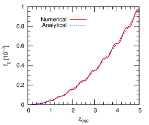
Figure 1: Evolution of the occupation number $f_{\chi}$ for the growing mode with $k=k_{\ast}$. The red solid line shows the numerical result while the blue dashed line shows the analytical result (23). Here we take $g_{S}=10^{-8}$ and $\beta_{\chi}=0.5$.

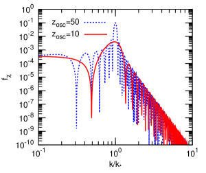
Figure 2: Distribution function $f_{\chi}$ in momentum space $(k/k_{\ast})$ at $z_{\rm osc}=10$ (the red solid line) and at $z_{\rm osc}=50$ (the blue dashed line). Here we take $g_{S}=10^{-8}$ and $\beta_{\chi}=0.5$.

In order to confirm the obtained results we numerically solve the equation of motion (11) and estimate the yield of $\chi$. As representative values we will take $m_{\phi}=1.5\times 10^{13}$ GeV and $\Phi=3.4\times 10^{19}$ GeV from now on. In Fig. 2 we show the evolution of the occupation number for the growing mode with $k=k_{\ast}$ in terms of the number of $\phi$ oscillation $z_{\rm osc}=m_{\phi}t/(2\pi)$ by taking $g_{S}=10^{-8}$ and $\beta_{\chi}=0.5$ (i.e., $m_{\chi}\simeq 0.43\,m_{\phi}$). It is seen that the analytical estimation in Eq. (23) successfully abstracts the characteristic behaviour of the occupation number, $f_{\chi}(t,k_{\ast})\propto t^{2}$.

The exact expression for the distribution function at ${\cal O}(g_{S}^{2})$ is obtained from Eqs. (19) and (21), which is given by

$$f_{\chi}(t,k) = \frac{g_{S}^{2}\,\Phi^{2}\,m_{\phi}^{2}\,m_{\chi}^{2}}{16\,\omega_{\chi}^{4}}I(t,\omega_{\chi},m_{\phi})\,,$$ (24)

where

$$I(t,\omega_{\chi},m_{\phi}) = \frac{2}{(m_{\phi}^{2}-4\,\omega_{\chi}^{2})^{2}}\Biggl{\{}3m_{\phi}^{2}+4\omega_{\chi}^{2}+(m_{\phi}^{2}-4\omega_{\chi}^{2})\cos(2m_{\phi}t)$$ (25)

$$\hskip 4.30554pt-2m_{\phi}\Bigl{[}(m_{\phi}+2\omega_{\chi})\cos\bigl{(}(m_{\phi}-2\omega_{\chi})t\bigr{)}+(m_{\phi}-2\omega_{\chi})\cos\bigl{(}(m_{\phi}+2\omega_{\chi})t\bigr{)}\Bigr{]}\Biggr{\}}\,.~{}~{}~{}~{}~{}~{}~{}$$

Fig. 2 shows the numerical results of the distribution functions at $z_{\rm osc}=10$ and $50$. We have confirmed that Eq. (24) agrees with the numerical results for the parameter choice in the figure. It is seen that $f_{\chi}$ has a peak at $k\simeq k_{\ast}$. For the case of $z_{\rm osc}=10$ the peak is located at the momentum slightly smaller than $k_{\ast}$ because of the effect of the oscillation terms, and such an effect become negligible for larger $z_{\rm osc}$. It is interesting to note that the modes with $k>k_{\ast}$ are produced, which are kinematically forbidden in the process where $\phi$ at rest decays into a pair of $\chi$. However, their occupation numbers are highly suppressed and it scales as $k^{-8}$ or $k^{-6}$ when $2z_{\rm osc}$ is integer or not, respectively. On the other hand, for the modes with $k\ll k_{\ast}$ the occupation number is independent on $k$ and they oscillate around a constant value. Furthermore, we can also see from Fig. 2 that the typical width of the peak in $f_{\chi}$ is inversely proportional to time.

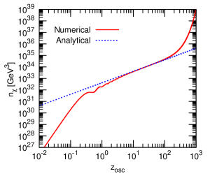
Figure 3: Evolution of the number density $n_{\chi}$ in terms of $z_{\rm osc}$. The red solid line shows the numerical result while the blue dashed line shows the analytical result (26). Here we take $g_{S}=10^{-8}$ and $\beta_{\chi}=0.5$.

The number density is then found at the leading order

$$n_{\chi}(t)\simeq\frac{g_{S}^{2}\,\Phi^{2}\,m_{\chi}^{2}\,\beta_{\chi}}{8\pi}\,t\,.$$ (26)

Here we have listed only the terms proportional to $t$ and neglected the oscillation terms. The derivation of Eq. (26) is explained in Appendix A. In Fig. 3 we compare Eq. (26) with the exact numerical result. First, we observe that the number density grows as $t^{4}$ initially, and there is a descrepancy between the leading ${\cal O}(g_{S}^{2})$ and numerical results. After a few coherent oscillations, however, the number density is approaching to the ${\cal O}(g_{S}^{2})$ result (26), and linearly grows in time with a small correction of oscillation. Moreover, it should be noted that the perturbative result (26) coincides with the naive result given in Eq. (6), and hence $n_{\chi}$ at the leading order can be estimated by the decays of non-relativistic $\phi$ into pairs of $\chi$ after a few oscillation. The same conclusion has been obtained in study of the narrow parametric resonance by using the method of the density matrix. [19] Finally, Fig. 3 also shows that the perturbative result breaks down for $z_{\rm osc}\gtrsim 100$. Therefore, we have clarified that the perturbative estimation (as well as the naive estimation in Sec. 2) of the yield can be applied only in the limited time interval.

3.2 Production of fermion

Next, we turn to consider the production of the Dirac fermion $\psi$. The equation of motion for $\psi$ is

$$\Bigl{[}i\,\gamma^{\mu}\,\partial_{\mu}-M_{\psi}(t)\Bigr{]}\psi(t,\vec{x})=0\,,$$ (27)

where $M_{\psi}(t)=g_{F}\,\phi(t)=m_{\psi}+g_{F}\,\Phi\,\cos(m_{\phi}t)$. We decompose $\psi$ as

$$\psi(t,\vec{x})=\int\frac{d^{3}k}{(2\pi)^{3/2}}\sum_{h}\left[u_{h}(t,\vec{k})\,\hat{b}_{h}(\vec{k})+v_{h}(t,\vec{k})\,\hat{d}_{h}^{\dagger}(-\vec{k})\right]\,e^{i\vec{k}\cdot\vec{x}}\,,$$ (28)

where the summation is taken over helicity $h=\pm$, and $v_{h}(t,\vec{k})=u_{h}^{c}(t,-\vec{k})$. $\hat{b}_{h}$ and $\hat{d}_{h}$ are annihilation operators of particle and anti-particle, respectively, and they satisfy the anti-commutation relations $\{\hat{b}_{h_{1}}(\vec{k}_{1}),\hat{b}_{h_{2}}^{\dagger}(\vec{k}_{2})\}=\{\hat{d}_{h_{1}}(\vec{k}_{1}),\hat{d}_{h_{2}}^{\dagger}(\vec{k}_{2})\}=\delta_{h_{1}h_{2}}\delta^{3}(\vec{k}_{1}-\vec{k}_{2})$. We write the wave function $u_{h}$ as

$$u_{h}(t,\vec{k})=\left(\begin{array}[]{c}P_{h}(t,k)\\ Q_{h}(t,k)\end{array}\right)\otimes\varphi_{h}(\vec{k})\,,$$ (31)

where the helicity eigenfunction satisfies $\vec{k}\,\varphi_{h}(\vec{k})=hk\,\varphi_{h}(\vec{k})$. Note that the mode functions $P_{h}$ and $Q_{h}$ obey the normalization condition $|P_{h}(t,k)|^{2}+|Q_{h}(t,k)|^{2}=1$. It is then found from Eq. (27) that the equation of motion $P_{h}$ is

$$\ddot{P}_{h}(t,k)+\tilde{\omega}_{k}^{2}(t)\,P_{h}(t,k)=0\,,$$ (32)

where $\tilde{\omega}_{k}$ is given by

$$\tilde{\omega}_{k}^{2}(t)=\omega_{k}^{2}(t)+i\,\dot{M}_{\psi}(t)=k^{2}+M_{\psi}^{2}(t)+i\,\dot{M}_{\psi}(t)\,.$$ (33)

As in the case of the scalar production, we assume a plain wave solution initially and impose the conditions

$$P_{h}(0,k)=\sqrt{\frac{\omega_{k}(0)+M_{\psi}(0)}{2\,\omega_{k}(0)}}\,,~{}~{}~{}~{}\dot{P}_{h}(0,k)=-i\,\omega_{k}(0)\,P_{h}(0,k)\,.$$ (34)

It is then seen that the equations of motion and the initial conditions for the $h=\pm$ states are the same, and so $P_{+}(t,k)=P_{-}(t,k)$. On the other hand, $Q_{h}$ is obtained from $P_{h}$ as

$$Q_{h}(t,k)=-i\,\frac{h}{k}\left[\dot{P}_{h}(t,k)+iM_{\psi}(t)\,P_{h}(t,k)\right]\,.$$ (35)

This means that $Q_{+}(t,k)=-\,Q_{-}(t,k)$. The distribution function of $\psi$ can be written in terms of the mode functions as (see, e.g., Ref. Garbrecht:2002pd)

$$f_{\psi}(t,k)=\frac{1}{2}-\frac{\Omega_{h}(t,k)}{2\,\omega_{k}(t)}\,,$$ (36)

where $\Omega_{h}$ is defined by

$$\Omega_{h}(t,k) = -hk\Bigl{[}P_{h}(t,k)Q_{h}^{\ast}(t,k)+Q_{h}(t,k)P_{h}^{\ast}(t,k)\Bigr{]}+M_{\psi}(t)\Bigl{[}\bigl{|}P_{h}(t,k)\bigr{|}^{2}-\bigl{|}Q_{h}(t,k)\bigr{|}^{2}\Bigr{]}$$ (37)

$$= -2\,\mbox{Im}\Bigl{[}P_{h}^{\ast}(t,k)\,\dot{P}_{h}(t,k)\Bigr{]}-M_{\psi}(t)\,.$$

This clearly shows that the distribution functions for two helicity states are exactly the same. Finally, the number density of $\psi$ is given by

$$n_{\psi}(t)=4\int\frac{d^{3}k}{(2\pi)^{3}}\,f_{\psi}(t,k)\,.$$ (38)

Here a factor of four counts the number of internal degrees of freedom of $\psi$.

We then turn to estimate the leading contribution to the yield of $\psi$ when $g_{F}$ is very small. Since $P_{+}=P_{-}$, the index $h$ will be implicit from now on. In order to solve Eq. (32) we express $P$ as

$$P(t,k)=\frac{A_{k}(t)}{\sqrt{2\,\tilde{\omega}_{k}(t)}}\,e^{-i\int_{0}^{t}dt_{1}\,\tilde{\omega}_{k}(t_{1})}+\frac{B_{k}(t)}{\sqrt{2\,\tilde{\omega}_{k}(t)}}\,e^{+i\int_{0}^{t}dt_{1}\,\tilde{\omega}_{k}(t_{1})}\,.$$ (39)

In this case the coefficients $A_{k}$ and $B_{k}$ obey the coupled equations

$$\dot{A}_{k}(t) = \frac{\dot{\tilde{\omega}}_{k}(t)}{2\,\tilde{\omega}_{k}(t)}\exp\left[+2i\int_{0}^{t}dt_{1}\,\tilde{\omega}_{k}(t_{1})\right]B_{k}(t)\,,$$ (40)

$$\dot{B}_{k}(t) = \frac{\dot{\tilde{\omega}}_{k}(t)}{2\,\tilde{\omega}_{k}(t)}\exp\left[-2i\int_{0}^{t}dt_{1}\,\tilde{\omega}_{k}(t_{1})\right]A_{k}(t)\,,$$ (41)

and their initial values are found from Eq. (34) as

$$A_{k}(0) = \Bigl{[}m_{\psi}+g_{F}\Phi+\bigl{(}\omega_{\psi}^{2}+2g_{F}\Phi m_{\psi}+g_{F}^{2}\Phi^{2}\bigr{)}^{1/2}\Bigr{]}^{1/2}\,,~{}~{}~{}B_{k}(0)=0\,,$$ (42)

where $\omega_{\psi}^{2}=k^{2}+m_{\psi}^{2}$ is the frequency of $\psi$ in the true vacuum $\Phi=0$. From now on let us find solutions of $A_{k}$ and $B_{k}$ in power series of coupling $g_{F}$ as we did in the $\chi$ production.

The leading term of $B_{k}$ is found to be ${\cal O}(g_{F})$, which can be obtained as

$$B_{k}(t) = \int_{0}^{t}dt_{1}\,\frac{\dot{\tilde{\omega}}_{k}(t_{1})}{2\,\tilde{\omega}_{k}(t_{1})}\,e^{-2i\int_{0}^{t_{1}}dt_{2}\,\tilde{\omega}_{k}(t_{2})}\,A_{k}(t_{1})=-i\,\frac{g_{F}\,\Phi\,m_{\phi}}{8\,\omega_{\psi}^{2}}\,A_{k}^{(0)}\,I^{\psi}_{1}(t,k)+{\cal O}(g_{F}^{2})\,,$$ (43)

where $A_{k}^{(0)}=\sqrt{\omega_{\psi}+m_{\psi}}$ denotes the ${\cal O}(g_{F}^{0})$ term of $A_{k}$ which is independent on time, and we have introduced

$$I^{\psi}_{1}(t,k)=\int_{0}^{t}dt_{1}\Bigr{[}(m_{\phi}-2m_{\psi})\,e^{i(m_{\phi}-2\omega_{\psi})t_{1}}+(m_{\phi}+2m_{\psi})\,e^{-i(m_{\phi}+2\omega_{\psi})t_{1}}\Bigl{]}\,.$$ (44)

Then, we can again see that $B_{k}$’s oscillate with time for all the modes expect for the mode with $\omega_{\psi}=m_{\phi}/2$, i.e., with the momentum

$$k_{\ast}=\frac{m_{\phi}}{2}\beta_{\psi}\,,$$ (45)

if $m_{\psi}<m_{\phi}/2$. Notice that it corresponds to the momentum of $\psi$ in the decay process $\phi\to\psi+\overline{\psi}$. For this growing mode we find that

$$B_{k_{\ast}}(t)=-i\,\frac{g_{F}\,\Phi\,A_{k_{\ast}}^{(0)}}{2\,m_{\phi}}\,(m_{\phi}-2\,m_{\psi})\,t+\cdots\,,$$ (46)

and increases linearly in time (with corrections of oscillations), which is consequence of the cancellation of phases between the $\phi$ oscillation and the frequency of a pair of $\psi$. Moreover, $A_{k_{\ast}}$ increases as $t^{2}$ at ${\cal O}(g_{F}^{2})$, which can be seen as follows: We find from Eq. (40) that

$$A_{k}(t) = A_{k}(0)+\int_{0}^{t}dt_{1}\,\frac{\dot{\tilde{\omega}}_{k}(t_{1})}{2\,\tilde{\omega}_{k}(t_{1})}\,e^{+2i\int_{0}^{t_{1}}dt_{2}\,\tilde{\omega}_{k}(t_{2})}\,B_{k}(t_{1})$$ (47)

$$= A_{k}(0)-i\,\frac{g_{F}\,\Phi\,m_{\phi}}{8\,\omega_{\psi}^{2}}\,I^{\psi}_{2}(t,k)+\cdots\,,$$

where

$$I^{\psi}_{2}(t,k)=\int_{0}^{t}dt_{1}\,\Bigl{[}(m_{\phi}-2m_{\psi})\,e^{i(m_{\phi}+2\omega_{\psi})t_{1}}+(m_{\phi}+2m_{\psi})\,e^{-i(m_{\phi}-2\omega_{\psi})t_{1}}\Bigr{]}\,B_{k}(t_{1})\,.$$ (48)

By using Eq. (46) $A_{k_{\ast}}$ is given by

$$A_{k_{\ast}}(t)=A_{k_{\ast}}(0)-\frac{g_{F}^{2}\,\Phi^{2}\,\beta_{\psi}^{2}\,A_{k_{\ast}}^{(0)}}{8}\,t^{2}+\cdots\,.$$ (49)

Therefore, the leading ${\cal O}(g_{F}^{2})$ contribution to the occupation number of the mode $k=k_{\ast}$ is found from Eqs. (36) and (37)

$$f_{\psi}(t,k_{\ast})\simeq\left(\frac{g_{F}\,\Phi\,\beta_{\psi}}{2}\right)^{2}\,t^{2}\,.$$ (50)

by neglecting the oscillation terms.

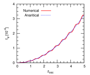
Figure 4: Evolution of the occupation number $f_{\psi}$ for the growing mode with $k=k_{\ast}$. The red solid line shows the numerical result while the blue dashed line shows the analytical result (50). Here we take $g_{F}=10^{-8}$ and $\beta_{\chi}=0.5$.

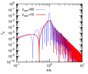
Figure 5: Distribution function $f_{\psi}$ in momentum space $(k/k_{\ast})$ at $z_{\rm osc}=10$ (the red solid line) and at $z_{\rm osc}=50$ (the blue dashed line). Here we take $g_{F}=10^{-8}$ and $\beta_{\chi}=0.5$.

We then compare the above result with the numerical solution of Eq. (32) which includes the higher order terms of $g_{F}$ and the oscillation terms. We show in Fig. 5 the evolution of the occupation number for the growing mode by taking $g_{F}=10^{-8}$ and $\beta_{\psi}=0.5$ (i.e., $m_{\psi}\simeq 0.43\,m_{\phi}$). We can see that the perturbative result (50) gives a good approximation for $f_{\psi}$, and it increases at $t^{2}$ with corrections from the oscillation terms.

The exact expression for the distribution function at the leading $g_{F}^{2}$ order is found from Eqs. (43) and (47) as

$$f_{\psi}(t,k) = \frac{g_{F}^{2}\,\Phi^{2}\,m_{\phi}^{2}\,k^{2}}{16\,\omega_{\psi}^{4}}I(t,\omega_{\psi},m_{\phi})\,,$$ (51)

where $I(t,\omega_{\psi},m_{\psi})$ is given by Eq. (25). Fig. 5 shows the numerical estimation of the distribution function $f_{\psi}$. Notice that we have confirmed that the analytical result in Eq. (51) agrees with the numerical one, as in the case of the scalar production. It is seen that $f_{\psi}$ has a peak at $k\simeq k_{\ast}$ and its height scales as $t^{2}$ as expected. Further, the figure shows that the typical width of the peak becomes narrow as $\Delta k(t)\propto 1/t$. It is also interesting to compare Eq. (24) with Eq. (51). The differences between $f_{\psi}$ and $f_{\chi}$ are in the prefactor ($k\leftrightarrow m_{\chi}$) and in the arguments of the function $I$. Because of these differences, $f_{\psi}$ for the modes $k\ll k_{\ast}$ does dependent on $k$ in contrast to scalar production and the suppression of $f_{\psi}$ for $k\gg k_{\ast}$ is relaxed. Moreover, the former difference provides the additional $\beta_{\psi}^{2}$ factor for the number density of produced $\psi$.

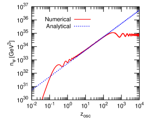
Figure 6: Evolution of the number density $n_{\psi}$ in terms of $z_{\rm osc}$. The red solid line shows the numerical result while the blue dashed line shows the analytical result (52). Here we take $g_{F}=10^{-8}$ and $\beta_{\psi}=0.5$.

As shown in Appendix A, the leading contribution to the number density of $\psi$ is given by

$$n_{\psi}(t)\simeq\frac{g_{F}^{2}\,\beta_{\psi}^{3}\,\Phi^{2}\,m_{\phi}^{2}}{8\pi}\,t\,,$$ (52)

by neglecting the oscillation terms. It is then found that the number density becomes independent on $m_{\psi}$ for $m_{\psi}\ll m_{\phi}$ (as long as $\Phi\ll{\langle\phi\rangle}$). Notice that it coincides with the naive result in Eq. (7).

In Fig. 6 the evolution of the number density $n_{\psi}$ is also shown. We can see that the numerical result is approaching to the analytical estimate (52) after a few oscillations of $\phi$. Therefore, the leading ${\cal O}(g_{F}^{2})$ contribution to the $\psi$ yield is also described by the decays of non-relativistic $\phi$ particles into pairs of $\psi$ and $\overline{\psi}$. However, it is also found from Fig. 6 that the $\mathcal{O}(g_{F}^{2})$ result in Eq. (52) breaks down in sufficiently later times, say $z_{\rm osc}\gtrsim 100$, as in the scalar production. This issue will be discussed in the next section.

4 Non-perturbative Corrections

We have so far estimated the leading contributions to the yields of $\chi$ and $\psi$ from the coherent oscillation. When the amplitude of the oscillation is small enough, the yields are induced at the order of ${\cal O}(g_{S,F}^{2})$. In this case there exists the growing mode with $k=k_{\ast}$ if $m_{\chi,\psi}<m_{\phi}/2$ and its occupation number grows at the rate $t^{2}$ after a small number of oscillations. The number density $n_{\chi,\psi}$ becomes proportional to $t$, which is consistent with the naive estimation in Eqs. (6) and (7) based on the decays of non-relativistic particles. It is, however, found that the perturbative result eventually fails to describe the evolution of the yield at later times.

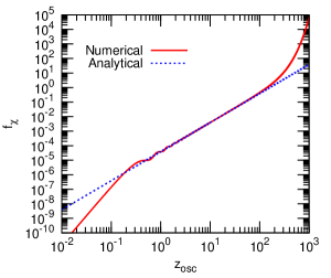
Figure 7: Same as Fig. 2 except for the range of $z_{\rm osc}$.

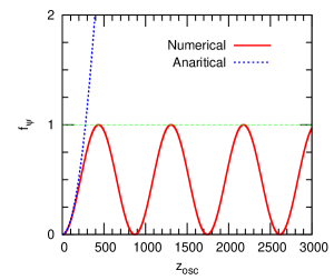
Figure 8: Same as Fig. 5 except for the range of $z_{\rm osc}$.

As for the $\chi$ production, Fig. 8 shows how the occupation number for the growing mode evolves at later epoch. We can see that $f_{\chi}(t,k_{\ast})$ starts to grow exponentially, which is different from the ${\cal O}(g^{2}_{S})$ result given in (23). As already pointed out in Ref. Kofman:1994rk, this discrepancy comes from the non-perturbative effect due to the narrow resonance at the preheating stage. Such an explosive production is reflected the statistical property of $\chi$, i.e., the effect of the Bose condensation. Then, the number density of $\chi$ also grows exponentially as also shown in Fig. 3. On the other hand, with regard to the $\psi$ production, the later evolution of $f_{\psi}(t,k_{\ast})$ is shown in Fig. 8. In this case the ${\cal O}(g^{2}_{F})$ result in (50) becomes inconsistent in the end and it oscillates between zero and unity. This oscillation behaviour had already been observed in Ref. Greene:1998nh, which is a consequence of the Pauli-blocking effect, i.e., $f_{\psi}$ is forbidden to exceed unity. Accordingly, the number density stops to grow at some point as also shown in Fig. 6.

The importance of these non-perturbative corrections have already been addressed in various cases of the preheating process. It should be stressed that such corrections become significant eventually even if the coupling constant $g_{S,F}$ is extremely small. In general, it is a difficult task to derive the analytical expression for the yield including the non-perturtative effect. The previous works [7, 9, 19] had investigated by using the knowledge of the Mathieu function, [20] since the solution of (11) is approximately given by this function. Here we utilize another method, the time averaging method, which is familiar in the study of the non-linear differential equations. [15] From now on we will demonstrate that the evolution of the occupation number for the growing mode can be successfully described by this method. Note that the time averaging method has already been used to describe the resonance structure of Mathieu function [6], where the authors have focused only on the scalar production, and have obtained the Mathieu characteristic exponent of the first instability band and Eq. (72) shown in below.

We will demonstrate below a simpler application of the time averaging method together with the method of variation of parameters. This allows us to clearly derive the analytical forms of the mode function and the occupation number for the growing mode. Furthermore, our approach is applicable not only to the scalar production but also to the fermion production as shown in below.

4.1 Growing mode of scalar

Let us recall the equation of motion for $\chi_{k}$ (11) for the growing mode $k=k_{\ast}$

$$\frac{d^{2}\chi_{k_{\ast}}}{d\tau^{2}}+\left[1+2\,q_{\chi}\,\sqrt{1-\beta_{\chi}^{2}}\,\cos(2\tau)+q_{\chi}^{2}\,\cos^{2}(2\tau)\right]\,\chi_{k_{\ast}}=0\,,$$ (53)

where we have introduced $\tau=m_{\phi}t/2$, and $q_{\chi}=2g_{S}\Phi/m_{\phi}$. We shall solve this equation by using the methods of variation of parameters and time averaging. For this purpose, we introduce $u_{1}$ and $u_{2}$ by

$$\chi_{k_{\ast}}(\tau)=y_{1}(\tau)\,u_{1}(\tau)+y_{2}(\tau)\,u_{2}(\tau)\,,$$ (54)

with the condition

$$y_{1}(\tau)\,\frac{du_{1}(\tau)}{d\tau}+y_{2}(\tau)\,\frac{du_{2}(\tau)}{d\tau}=0\,,$$ (55)

where $y_{1}=\cos\tau$ and $y_{2}=\sin\tau$ are the solutions for Eq. (53) with $q_{\chi}=0$. We then obtain the equations for $u_{1}$ and $u_{2}$ as

$$\frac{d}{d\tau}\left(\begin{array}[]{c}u_{1}\\ u_{2}\end{array}\right) = \left[2\,q_{\chi}\,\sqrt{1-\beta_{\chi}^{2}}\,\cos(2\tau)+q^{2}_{\chi}\,\cos^{2}(2\tau)\right]$$ (63)

$$\times\left(\begin{array}[]{c c}\sin\tau\,\cos\tau&\sin^{2}\tau\\ -\cos^{2}\tau&-\sin\tau\,\cos\tau\end{array}\right)\left(\begin{array}[]{c}u_{1}\\ u_{2}\end{array}\right)\,.$$

Now we are interested in the characteristic behaviour of $\chi_{k_{\ast}}$ due to the non-perturbative effect and, as shown below, its typical time scale is given by $\tau\sim 1/q_{\chi}$ which is much longer than the period of the $\phi$ oscillation in the weak coupling limit (say, $q_{\chi}\ll 1$). In this situation we can apply the time averaging method which extract the underlying behaviour over a long time scale by integrating out the effects of the rapid $\phi$ oscillations. The $u_{1}$ and $u_{2}$ averaged over the oscillation period are denoted by $\overline{u}_{1}$ and $\overline{u}_{2}$, and they satisfy

$$\frac{d}{d\tau}\left(\begin{array}[]{c}\overline{u}_{1}\\ \overline{u}_{2}\end{array}\right)=-\frac{q_{\chi}\sqrt{1-\beta_{\chi}^{2}}}{2}\left(\begin{array}[]{c c}0&1\\ 1&0\end{array}\right)\left(\begin{array}[]{c}\overline{u}_{1}\\ \overline{u}_{2}\end{array}\right)\,.$$ (70)

Here and hereafter, we neglect the contributions of higher order of $q_{\chi}$. By using the initial conditions (15) at ${\cal O}(g_{S}^{0})$, $\chi_{k_{\ast}}$ after the time averaging is obtained as

$$\chi_{k_{\ast}}(\tau) = y_{1}(\tau)\overline{u}_{1}(\tau)+y_{2}(\tau)\overline{u}_{2}(\tau)$$ (71)

$$= \frac{1}{\sqrt{m_{\phi}}}\left[e^{-i\tau}\,\cosh\left(\frac{q_{\chi}\sqrt{1-\beta_{\chi}^{2}}}{2}\tau\right)+i\,e^{+i\tau}\,\sinh\left(\frac{q_{\chi}\sqrt{1-\beta_{\chi}^{2}}}{2}\tau\right)\right]\,.$$

Finally, Eq.(13) gives the occupation number for the growing mode with $k=k_{\ast}$ as

$$f_{\chi}(t,k_{\ast})=\sinh^{2}\left(\frac{g_{S}\Phi}{2}\,\sqrt{1-\beta_{\chi}^{2}}\,t\right)=\sinh^{2}\left(\frac{g_{S}\,\Phi\,m_{\chi}}{m_{\phi}}\,t\right)\,.$$ (72)

We have checked that the obtained result can describe the exact numerical one in Fig. 8 apart from tiny corrections of oscillation. Interestingly, this correctly reproduces the initial behaviour in Eq. (23) for $1/m_{\phi}\ll t\ll t_{\rm cr}=m_{\phi}/(g_{S}\Phi m_{\chi})$. When $g_{S}=10^{-8}$ and $m_{\chi}\simeq 0.43m_{\phi}$ shown in Fig. 8, the critical time is estimated to be $z_{\rm cr}\simeq 160$ (i.e., $t_{\rm cr}\simeq 7\times 10^{-11}\mbox{~{}GeV}^{-1}$). Note that the exact numerical estimation of $f_{\chi}$ shows $f_{\chi}\propto t^{4}$ for the beginnings of production (within one oscillation), which can not be explained by this result. On the other hand, for $t\gg t_{\rm cr}$, the occupation number grows exponentially as $\exp(2g_{S}\Phi m_{\chi}t/m_{\phi})$. This exponent is consistent with the result from the narrow parametric resonance. [7] Notice again that such non-perturbative correction becomes significant for $t\gtrsim t_{\rm cr}$ even if the coupling $g_{S}$ is extremely small. Accordingly, the number density starts to grow exponentially at $t\simeq t_{\rm cr}$.

It is important to note that the mode function for the growing mode in Eq. (71) satisfies the exact scaling property [16] in its time evolution, which is a consequence of the periodicity of the $\phi$ oscillation. To see this point, let us first recall the exact equation of motion for $\chi_{k}$ in Eq. (11) and denote by $\chi_{k}^{(1)}(t)$ and $\chi_{k}^{(2)}(t)$ its two linearly independent solutions with the initial conditions $\chi_{k}^{(1)}(0)=\dot{\chi}_{k}^{(2)}(0)=1$ and $\dot{\chi}_{k}^{(1)}(0)=\chi_{k}^{(2)}(0)=0$. In this case, $\chi_{k}$ can be written without loss of generality as

$$\chi_{k}(t)=\chi_{k}(0)\left[\chi_{k}^{(1)}(t)-i\omega_{k}(0)\chi_{k}^{(2)}(t)\right]\,.$$ (73)

Due to the periodicity of $\omega_{k}(t)$, the independent solutions satisfy the exact scaling property [16]

$$\left(\begin{array}[]{c}\chi_{k}^{(1)}(t+T)\\ \chi_{k}^{(2)}(t+T)\end{array}\right)=\left(\begin{array}[]{c c}\chi_{k}^{(1)}(T)&\dot{\chi}_{k}^{(1)}(T)\\ \chi_{k}^{(2)}(T)&\dot{\chi}_{k}^{(2)}(T)\end{array}\right)\left(\begin{array}[]{c}\chi_{k}^{(1)}(t)\\ \chi_{k}^{(2)}(t)\end{array}\right)\,,$$ (80)

where $T$ is an oscillation period of $\phi(t)$ (${\it i.e.},\,\omega_{k}(t+T)=\omega_{k}(t)$). This shows that we can extrapolate the mode function at $t=nT$ by using the solution at $t=T$ recursively. From this exact property, the occupation number of $\chi$ at the time $t=nT$ is written by

$$f_{\chi}(nT,k) = \frac{1}{4\omega_{k}^{2}(T)}\left(\frac{\sinh\left(nD\right)}{\sinh\left(D\right)}\right)^{2}\left(\dot{\chi}_{k}^{(1)}(T)+\omega_{k}^{2}(T)\chi_{k}^{(2)}(T)\right)^{2}$$ (81)

$$= \left[\frac{\sinh\left(nD\right)}{\sinh\left(\left(n-1\right)D\right)}\right]^{2}f_{\chi}\bigl{(}(n-1)T,k\bigr{)}\,,$$

where $D\equiv\cosh^{-1}(\chi_{k}^{(1)}(T))$. Therefore, the occupation number at $t=nT$ can be obtained by using the mode function at $t=T$.

Now, we examine whether the occupation number for the growing mode by the time averaging method (71) satisfy these scaling properties or not. It should be noted that our result can be written as Eq.(73) with

$$\chi_{k_{\ast}}^{(1)}(t) = \cosh\left(\frac{g_{S}\,\Phi\,m_{\chi}}{m_{\phi}}t\right)\cos\left(\frac{m_{\phi}t}{2}\right)-\sinh\left(\frac{g_{S}\,\Phi\,m_{\chi}}{m_{\phi}}t\right)\sin\left(\frac{m_{\phi}t}{2}\right)\,,$$ (82)

$$\chi_{k_{\ast}}^{(2)}(t) = \frac{2}{m_{\phi}}\left[\cosh\left(\frac{g_{S}\,\Phi\,m_{\chi}}{m_{\phi}}t\right)\sin\left(\frac{m_{\phi}t}{2}\right)-\sinh\left(\frac{g_{S}\,\Phi\,m_{\chi}}{m_{\phi}}t\right)\cos\left(\frac{m_{\phi}t}{2}\right)\right]\,.$$ (83)

Here we have taken the mode function at the initial time as a free field. We can show that these functions satisfy the exact scaling property (80). See the details in Ref. AN. Moreover, substituting Eqs. (82) and (83) into Eq. (81), we obtain the occupation number at $t=nT$ with exact scaling property as

$$f_{\chi}(nT,k_{\ast})=\sinh^{2}\left(\frac{g_{S}\,\Phi\,m_{\chi}}{m_{\phi}}\,nT\right)\,.$$ (84)

This result is consistent with Eq. (72). Therefore, the analytical result for the occupation number obtained by the time averaging method can satisfy the exact relation in its evolution coming from the periodicity of the $\phi$ oscillation.

4.2 Growing mode of fermion

Next, we turn to consider the occupation number of $\psi$ with $k=k_{\ast}$ at later time. The equation of motion for the mode function is now given by

$$\frac{d^{2}P(\tau)}{d\tau^{2}}+\left[1+2\,q_{\psi}\,\sqrt{1-\beta_{\psi}^{2}}\,\cos(2\tau)-2i\,q_{\psi}\,\sin(2\tau)+q_{\psi}^{2}\cos^{2}(2\tau)\right]P(\tau)=0\,,$$ (85)

where $q_{\psi}=2g_{F}\Phi/m_{\phi}$. As before, we shall use the method of variation of parameters and write

$$P(\tau)=y_{1}(\tau)\,u_{1}(\tau)+y_{2}(\tau)\,u_{2}(\tau)\,,$$ (86)

where $y_{1}=\cos\tau$ and $y_{2}=\sin\tau$ are the solutions of (85) for the case $q_{\psi}=0$. Together with the condition (55) we obtain the equations for $u_{1}$ and $u_{2}$ as

$$\frac{d}{d\tau}\left(\begin{array}[]{c}u_{1}\\ u_{2}\end{array}\right) = \left[2\,q_{\psi}\,\sqrt{1-\beta_{\psi}^{2}}\,\cos(2\tau)-2i\,q_{\psi}\,\sin(2\tau)+q_{\psi}^{2}\cos^{2}(2\tau)\right]$$ (94)

$$\times\left(\begin{array}[]{c c}\sin\tau\,\cos\tau&\sin^{2}\tau\\ -\cos^{2}\tau&-\sin\tau\,\cos\tau\end{array}\right)\left(\begin{array}[]{c}u_{1}\\ u_{2}\end{array}\right)\,.$$

By integrating over the period of the $\phi$ oscillation, the averaged $\overline{u}_{1}$ and $\overline{u}_{2}$ satisfy

$$\frac{d}{d\tau}\left(\begin{array}[]{c}\overline{u}_{1}\\ \overline{u}_{2}\end{array}\right)=-\frac{1}{2}\left(\begin{array}[]{c c}iq_{\psi}&q_{\psi}\sqrt{1-\beta_{\psi}^{2}}\\ q_{\psi}\sqrt{1-\beta_{\psi}^{2}}&-iq_{\psi}\end{array}\right)\left(\begin{array}[]{c}\overline{u}_{1}\\ \overline{u}_{2}\end{array}\right)\,.$$ (101)

From the initial conditions (34) at the leading order, namely, $P(0)=(1+({1-\beta_{\psi}^{2}})^{1/2})^{1/2}$ and $dP(0)/d\tau=-iP(0)$, we obtain the solution

$$P(\tau)=P(0)\left[e^{-i\tau}\,\cos\left(\frac{q_{\psi}\beta_{\psi}\tau}{2}\right)+i\frac{\sqrt{1-\beta_{\psi}^{2}}-1}{\beta_{\psi}}\,e^{i\tau}\sin\left(\frac{q_{\psi}\beta_{\psi}\tau}{2}\right)\right]\,.$$ (102)

It is then found from (36) that the occupation number for the growing mode is given by

$$f_{\psi}(t,k_{\ast})=\sin^{2}\left(\frac{q_{\psi}\,\beta_{\psi}\,\tau}{2}\right)=\sin^{2}\left(\frac{g_{F}\,\Phi\,\beta_{\psi}}{2}\,t\right)\,.$$ (103)

Note again that this reproduces the initial behaviour in Eq. (50) for $t\ll t_{\rm cr}=2/(g_{F}\Phi\beta_{\psi})$, as in the scalar production. In Fig. 8, $z_{\rm cr}$ is around 300 when $g_{F}=10^{-8}$ and $\beta_{\psi}=0.5$. On the other hand, for $t\gg t_{\rm cr}$, the occupation number oscillates around $f_{\psi}=1/2$ and does not exceed one, which should be contrast to the scalar production. This behaviour reflects the Pauli blocking effect of the produced fermion $\psi$. As a result, the number density of $\psi$ stops to grow at $t\simeq t_{\rm cr}$ even if the coupling $g_{F}$ is extremely small.

As in the case of scalar production, it can be confirmed that the solution in Eq. (102) satisfies the exact relation between the mode functions at different times. For all the mode $P(t,k)$ can be written as

$$P(t,k)=P(0,k)\left[P^{(1)}(t,k)-i\,\omega_{k}(0)P^{(2)}(t,k)\right]\,.$$ (104)

Here $P^{(1,2)}(t,k)$ correspond to linear independent solutions of the equation of motion with the initial conditions $P^{(1)}(0,k)=\dot{P}^{(2)}(0,k)=1$ and $\dot{P}^{(1)}(0,k)=P^{(2)}(0,k)=0$. These solutions satisfy the same scaling property as Eq. (80) by replacing $\chi_{k}^{(1,2)}$ into $P^{(1,2)}$ and the occupation number of $\psi$ at $t=nT$ is obtained by same manner as

$$f_{\psi}(nT,k) = \frac{k^{2}}{\omega_{k}(T)^{2}}\frac{\sin^{2}(n\,d)}{\sin^{2}(d)}\left[{\rm Im}P^{(1)}(T,k)\right]^{2}$$ (105)

$$= \left[\frac{\sin(n\,d)}{\sin\left(\left(n-1\right)\,d\right)}\right]^{2}f_{\psi}\bigl{(}(n-1)T,k\bigr{)}\,,$$

where $d\equiv\cos^{-1}\left({\rm Re}P^{(1)}(T)\right)$. This equation has already been presented in Ref. Greene:1998nh, however, the estimation of $P^{(1)}(T,k)$ is essential to obtain $f_{\psi}(nT,k)$ by using Eq. (105).

Now the time averaging method gives us the analytical expression of $P(t,k_{\ast})$ for the growing mode. Therefore, we can estimate $f_{\psi}(nT,k_{\ast})$ analytically by taking $P^{(1)}(t,k_{\ast})$ and $P^{(2)}(t,k_{\ast})$ as

$$P^{(1)}(t,k_{\ast}) = \cos\left(\frac{m_{\phi}t}{2}\right)\left[\cos\left(\frac{g_{F}\,\Phi\,\beta_{\psi}}{2}t\right)-i\frac{1}{\beta_{\psi}}\sin\left(\frac{g_{F}\,\Phi\,\beta_{\psi}}{2}t\right)\right]$$ (106)

$$-\frac{\sqrt{1-\beta_{\psi}^{2}}}{\beta_{\psi}}\sin\left(\frac{m_{\phi}t}{2}\right)\sin\left(\frac{g_{F}\,\Phi\,\beta_{\psi}}{2}t\right)\,,$$

$$P^{(2)}(t,k_{\ast}) = -\frac{2}{m_{\phi}}\frac{\sqrt{1-\beta_{\psi}^{2}}}{\beta_{\psi}}\cos\left(\frac{m_{\phi}t}{2}\right)\sin\left(\frac{g_{F}\,\Phi\,\beta_{\psi}}{2}t\right)$$ (107)

$$+\frac{2}{m_{\phi}}\sin\left(\frac{m_{\phi}t}{2}\right)\left[\cos\left(\frac{g_{F}\,\Phi\,\beta_{\psi}}{2}t\right)+i\frac{1}{\beta_{\psi}}\sin\left(\frac{g_{F}\,\Phi\,\beta_{\psi}}{2}t\right)\right]\,.$$

Substituting Eq. (106) into Eq. (105), we obtain the occupation number at $t=nT$ with exact scaling property as

$$f_{\psi}(nT,k_{\ast})=\sin^{2}\left(\frac{g_{F}\,\Phi\,\beta_{\psi}}{2}nT\right)\,.$$ (108)

Similar to the scalar production this result is consistent with (103) obtained by the time averaging method.

Thus, we conclude that the results by the time averaging method can not only abstract the characteristic evolution due to the non-perturbative correction but also satisfy the exact scaling property in terms of oscillation period of $\phi$.

5 Conclusion

We have investigated the particle production from the coherent oscillation by using the method based on the Bogolyubov transformation. For the case when the coupling constants of the oscillating field are very small, we have obtained the leading contributions to the distribution functions and the number densities of the produced particles.

When the amplitude of the oscillation is small ($\Phi\ll{\langle\phi\rangle}$), the leading contributions to the yields are found to be ${\cal O}(g_{S,F}^{2})$. We have presented the exact expressions for the distribution functions of the produced $\chi$ and $\psi$ at the ${\cal O}(g_{S,F}^{2})$ order. It has been shown that there exists the growing mode with $k=k_{\ast}$ if $m_{\chi,\psi}<m_{\phi}/2$, and its occupation number increases at the rate $t^{2}$ after sufficient numbers of the oscillation. The distribution function has a peak at $k\simeq k_{\ast}$ and the width of the peak decreases at the rate $1/t$. As a result, the number density of produced particles is proportional to $t$. The expression for the number density is found to be consistent with the one obtained by assuming that the coherent oscillation is a correction of non-relativistic scalar particles and the decay process is a main source of the particle production.

We have found that the above perturbative results fail to describe the exact ones for sufficient late times since the non-perturbative correction becomes significant even when the coupling constants are extremely small. Indeed, the occupation number of $\chi$ for the growing mode increases exponentially while that of $\psi$ oscillates around $1/2$. These distinctive features represent the statistical properties of the produced particles, i.e., the effects of the Bose condensation for the scalar production or the Pauli blocking for the fermion production. Due to these non-perturbative effects, the explosive production of $\chi$ happens while the production of $\psi$ becomes insignificant for late times. To handle with these non-perturbative effects we have used the time averaging method, and have successfully described the evolution of the occupation number for the growing mode. This method works well because the typical time scale of the evolution is much longer than the rapid $\phi$ oscillation. Furthermore, we have shown that the results obtained by the time averaging method satisfies the exact scaling properties in Ref.Mostepanenko:1974, which also gives the justification of the use of the time averaging method.

Throughout this analysis, we have neglected the back-reaction effect of the produced particles in the estimation of the yields. When the occupation number of these particles is close to unity, such an effect should be taken into account. In addition to this, the inclusion of the expansion of the universe is also necessary to reveal the reheating/preheating processes in the inflationary universe. These issue will be discussed in elsewhere [17].

Appendix A Derivations of Eqs. (26) and (52)

We show here the derivations of the number densities $n_{\chi}$ and $n_{\psi}$ at the leading order given in Eqs. (26) and (52). Let us first consider Eq. (26). It is found from Eqs. (19) and (21) that the leading $\mathcal{O}(g_{S}^{2})$ contribution to $n_{\chi}$ is given by

$$n_{\chi}(t) = \frac{g_{S}^{2}\,\Phi^{2}\,m_{\chi}^{2}\,m_{\phi}^{2}}{8\pi^{2}}\,K_{\chi}(t)\,,$$ (109)

where

$$K_{\chi}(t)=\int_{0}^{t}dt_{1}\,\sin(m_{\phi}t_{1})\int_{0}^{t}dt_{2}\,\sin(m_{\phi}t_{2})\,J_{\chi}(\Delta t)\,,$$ (110)

$$J_{\chi}(\Delta t)=\int_{0}^{\infty}dk\,\frac{k^{2}}{\omega_{\chi}^{4}}\,\cos(2\omega_{\chi}\Delta t)\,,$$ (111)

with $\Delta t=t_{2}-t_{1}$. The integration in Eq. (111) can be done as

$$J_{\chi}(\Delta t) = \frac{\pi}{4m_{\chi}}\left[1+4\,m_{\chi}^{2}\Delta t^{2}-4\,m_{\chi}|\Delta t|\,\mbox{${}_{1}$$F_{2}$}\left(-\frac{1}{2};1,\frac{3}{2};-m_{\chi}^{2}\Delta t^{2}\right)\right]\,,$$ (112)

where ${}_{1}F_{2}(a;b,c;x)$ is the generalized hypergeometric function. We then expand $J_{\chi}$ in terms of $m_{\chi}$ as

$$J_{\chi}(\Delta t)=\frac{\pi}{m_{\chi}}\left[\frac{1}{4}+(\Delta tm_{\chi})^{2}-{\left|\Delta t\right|}m_{\chi}\sum_{n=0}^{\infty}\frac{(-1)^{n+1}}{(4n^{2}-1)(n!)^{2}}(\Delta t\,m_{\chi})^{2n}\right]\,.$$ (113)

Now, we can perform the integrations of $t_{1}$ and $t_{2}$ in (110) as

$$K_{\chi}(t) = \frac{\pi}{m_{\phi}^{2}}\,t\,\left[1-2r_{\chi}^{2}-2r_{\chi}^{4}-4r_{\chi}^{6}-10r_{\chi}^{8}+\mathcal{O}(r_{\chi}^{10})\right]+...$$ (114)

$$\simeq \frac{\pi}{m_{\phi}^{2}}\,t\,\beta_{\chi}+...\,,$$

where $r_{\chi}=m_{\chi}/m_{\phi}$. Notice that we we have only listed the terms proportional to $t$ and dropped off the oscillation terms. Finally, we obtain the number density up to $\mathcal{O}(g_{S}^{2})$ as Eq. (26)

$$n_{\chi}(t) = \frac{g_{S}^{2}\,\Phi^{2}\,m_{\chi}^{2}\,m_{\phi}^{2}}{8\pi^{2}}\,K_{\chi}(t)\simeq\frac{g_{S}^{2}\,\Phi^{2}\,m_{\chi}^{2}\,\beta_{\chi}}{8\pi}\,t\,,$$ (115)

by neglecting the oscillation terms.

Next, we turn to consider Eq. (52). As in the case of the scalar production, the leading ${\cal O}(g_{F}^{2})$ contribution to the number density of $\psi$ is given by

$$n_{\psi}(t) = 4\,\frac{g_{F}^{2}\,\Phi^{2}\,m_{\phi}^{2}}{8\pi^{2}}\,K_{\psi}(t)\,,$$ (116)

where a prefactor 4 counts the internal degrees of freedom of $\psi$ and

$$K_{\psi}(t)=\int_{0}^{t}dt_{1}\,\sin(m_{\phi}t_{1})\int_{0}^{t}dt_{2}\,\sin(m_{\phi}t_{2})\,J_{\psi}(\Delta t)\,,$$ (117)

$$J_{\psi}(\Delta t)=\int_{0}^{\infty}dk\,\frac{k^{4}}{\omega_{\psi}^{4}}\,\cos(2\omega_{\psi}\Delta t)\,.$$ (118)

Notice that, comparing with Eq. (112), the integrand of $J_{\psi}$ has an extra factor $k^{2}$.

When $m_{\psi}=0$, we first integrate $t_{1}$ and $t_{2}$ in $K_{\psi}$ and then the $k$ integration in $J_{\psi}$ gives

$$K_{\psi}(t) = \frac{\pi t}{4}\left(1-\frac{\sin 2m_{\phi}t}{2m_{\phi}t}\right)\,.$$ (119)

On the other hand, when $m_{\psi}\neq 0$, we first estimate $J_{\psi}(\Delta t)$ as

$$J_{\psi}(\Delta t) = -\frac{\pi m_{\psi}}{4}\left[3+4m_{\psi}^{2}\Delta t^{2}-6m_{\psi}{\left|\Delta t\right|}{}_{1}F_{2}\left(-\frac{1}{2};\frac{3}{2},2;-m_{\psi}^{2}\Delta t^{2}\right)\right]$$ (120)

$$= -\frac{\pi m_{\psi}}{4}\left[3+4m_{\psi}^{2}\Delta t^{2}-6m_{\psi}{\left|\Delta t\right|}\sum_{n=0}^{\infty}\frac{(-1)^{n+1}}{(4n^{2}-1)(n+1)(n!)^{2}}(\Delta t\,m_{\psi})^{2n}\right]\,,~{}~{}~{}$$

After the integrations over $t_{1}$ and $t_{2}$ we find apart from the oscillation terms

$$K_{\psi}(t)=\frac{\pi}{2}t\left[-3r_{\psi}^{2}+3r_{\psi}^{4}+4r_{\psi}^{6}+3r_{\psi}^{8}+{\cal O}(r_{\psi}^{10})\right]+\dots\,,$$ (121)

where $r_{\psi}=m_{\psi}/m_{\phi}$. Combining the above two cases, we obtain

$$K_{\psi}(t) = \frac{\pi}{4}t\left[1-6r_{\psi}^{2}+6r_{\psi}^{4}+4r_{\psi}^{6}+6r_{\psi}^{8}+{\cal O}(r_{\psi}^{10})\right]+\dots$$ (122)

$$\simeq \frac{\pi}{4}t\beta_{\psi}^{3}+\dots\,,$$

which gives Eq. (52)

$$n_{\psi}(t)\simeq\frac{g_{F}^{2}\,\beta_{\psi}^{3}\,\Phi^{2}\,m_{\phi}^{2}}{8\pi}\,t\,,$$ (123)

by neglecting the oscillation terms.

References

- [1] A. D. Linde, Phys. Lett. B 108 (1982), 389; A. Albrecht and P. J. Steinhardt, Phys. Rev. Lett. 48 (1982), 1220.
- [2] For example, see A. D. Linde, Particle Physics and Inflationary Universe, (Addison-Wesley, Reading, MA, 1990).
- [3] D. Larson et al., arXiv:1001.4635 [astro-ph.CO].
- [4] M. S. Turner, Phys. Rev. D 28, 1243 (1983); J. Preskill and M. B. Wise and F. Wilczek, Phys. Lett. B 120, 127 (1983); L. F. Abbott and P. Sikivie, Phys. Lett. B 120, 133 (1983)
- [5] A. J. Albrecht, P. J. Steinhardt, M. S. Turner and F. Wilczek, Phys. Rev. Lett. 48 (1982), 1437; L. F. Abbott, E. Farhi and M. B. Wise, Phys. Lett. B 117 (1982), 29; A. D. Dolgov and A. D. Linde, Phys. Lett. B 116 (1982), 329.
- [6] J. H. Traschen and R. H. Brandenberger, Phys. Rev. D 42 (1990), 2491; Y. Shtanov, J. H. Traschen and R. H. Brandenberger, Phys. Rev. D 51 (1995), 5438 [arXiv:hep-ph/9407247].
- [7] L. Kofman, A. D. Linde and A. A. Starobinsky, Phys. Rev. Lett. 73 (1994), 3195 [arXiv:hep-th/9405187]; L. Kofman, A. D. Linde and A. A. Starobinsky, Phys. Rev. D 56 (1997), 3258 [arXiv:hep-ph/9704452].
- [8] D. Boyanovsky, H. J. de Vega, R. Holman, D. S. Lee and A. Singh, Phys. Rev. D 51 (1995), 4419 [arXiv:hep-ph/9408214]; D. Boyanovsky, M. D’Attanasio, H. J. de Vega, R. Holman and D. S. Lee, Phys. Rev. D 52 (1995), 6805 [arXiv:hep-ph/9507414].
- [9] M. Yoshimura, Prog. Theor. Phys. 94 (1995), 873 [arXiv:hep-th/9506176]; H. Fujisaki, K. Kumekawa, M. Yamaguchi and M. Yoshimura, Phys. Rev. D 53 (1996), 6805 [arXiv:hep-ph/9508378]; H. Fujisaki, K. Kumekawa, M. Yamaguchi and M. Yoshimura, Phys. Rev. D 54 (1996), 2494 [arXiv:hep-ph/9511381].
- [10] A. D. Dolgov and D. P. Kirilova, Sov. J. Nucl. Phys. 51(1990), 172 [Yad. Fiz. 51, 273 (1990)].
- [11] J. Baacke, K. Heitmann and C. Patzold, Phys. Rev. D 58 (1998), 125013 [arXiv:hep-ph/9806205].
- [12] P. B. Greene and L. Kofman, Phys. Lett. B 448 (1999), 6 [arXiv:hep-ph/9807339]; P. B. Greene and L. Kofman, Phys. Rev. D 62 (2000), 123516 [arXiv:hep-ph/0003018].
- [13] N. N. Bogolyubov, Sov. Phys. JETP 7, 41 (1958) [Zh. Eksp. Teor. Fiz. 34, 58 (1958 FRPHA,6,399-404.1961)]; Y. B. Zeldovich and A. A. Starobinsky, Sov. Phys. JETP 34, 1159 (1972) [Zh. Eksp. Teor. Fiz. 61, 2161 (1971)]; C. Pathinayake and L. H. Ford, Phys. Rev. D 35, 3709 (1987).
- [14] For example, see N. D. Birrell and P. C. .W. Davies, Quantum fields in curved space, Cambridge University Press, Cambridge, 1982.
- [15] A. H. Nayfeh, D. T. Mook, Nonlinear Oscillations, Wiley Classic Library, Wiley, 1995.
- [16] V. M. Mostepanenko and V. M. Frolov, Yad. Fiz. 19, 1974, 885.
- [17] T. Asaka and H. Nagao, in preparation.
- [18] B. Garbrecht, T. Prokopec and M. G. Schmidt, Eur. Phys. J. C 38, 135 (2004) [arXiv:hep-th/0211219].
- [19] M. Yoshimura, arXiv:hep-ph/9603356.
- [20] N. W. Mac Lauchlan, Theory and Application of Mathieu functions (Dover, New York, 1961).