The complex structure of HH 110 as revealed from Integral Field Spectroscopy

Abstract

HH 110 is a rather peculiar Herbig-Haro object in Orion that originates due to the deflection of another jet (HH 270) by a dense molecular clump, instead of being directly ejected from a young stellar object. Here we present new results on the kinematics and physical conditions of HH 110 based on Integral Field Spectroscopy. The 3D spectral data cover the whole outflow extent ($\sim$ 4.5 arcmin, $\simeq$ 0.6 pc at a distance of 460 pc) in the spectral range 6500–7000 Å. We built emission-line intensity maps of H$\alpha$, [N ii] and [S ii] and of their radial velocity channels. Furthermore, we analysed the spatial distribution of the excitation and electron density from [N ii]/H$\alpha$, [S ii]/H$\alpha$, and [S ii]6716/6731 integrated line-ratio maps, as well as their behaviour as a function of velocity, from line-ratio channel maps. Our results fully reproduce the morphology and kinematics obtained from previous imaging and long-slit data. In addition, the IFS data revealed, for the first time, the complex spatial distribution of the physical conditions (excitation and density) in the whole jet, and their behaviour as a function of the kinematics. The results here derived give further support to the more recent model simulations that involve deflection of a pulsed jet propagating in an inhomogeneous ambient medium. The IFS data give richer information than that provided by current model simulations or laboratory jet experiments. Hence, they could provide valuable clues to constrain the space parameters in future theoretical works.

1 Introduction

HH 110 is a Herbig-Haro (HH) jet emerging from the southern edge of the L1617 dark cloud in the Orion B complex. Both observational and theoretical works have been carried out since its discovery by Reipurth & Olberg (1991), because unlike most of the well-known stellar jets, HH 110 has a peculiar morphology, among other properties. The morphology of HH 110 in the H$\alpha$ and [S ii] lines is very complex, starting in a collimated chain of knots. The emission away from the collimated region has a more chaotic structure and widens within a cone of unusually large opening angle ($\sim 10^{\circ}$). HH 110 appreciable wiggles along the $\sim$ 4 arcmin jet length. The knots are all embedded in fainter emitting gas, which outlines the whole flow, more reminiscent of a turbulent outflow. Most of the knots detected in ground-based images are spatially resolved into several components in the higher spatial resolution HST images (see e. g. Hartigan et al., 2009). The transverse cross-section of HH 110 shows a significant asymmetry, the eastern border is sharp and poorly resolved, whereas the strong knotty emission mostly appears towards the western side. HH 110 is the only known HH that shows a faint filament of emission lying parallel at $\sim$ 10 arcsec to the east of the northern A-C knots, which probably represents a weak secondary or even a fossil flow channel (Reipurth & Olberg, 1991). Attempts to find the driving source of HH 110 have failed at optical, near infrared and radio continuum wavelengths.

A scenario that accounts for the singular morphology of HH 110 was first outlined by Reipurth, Raga & Heathcote (1996). These authors proposed that HH 110 originates from the deflection (deflection angle $\simeq 60^{\circ}$) of the adjacent HH 270 jet through a grazing collision with a dense molecular clump of gas. The feasibility of this scenario has been further reinforced from the results of numerical simulations, which model the emission arising from the collision of a jet with a dense molecular clump (see Raga et al., 2002 and references therein). In addition, analysis of further data are also in agreement with this scenario. First, a high-density clump of gas around the region where the HH 270 jet changes its direction to emerge as HH 110 has been detected through high-density tracer molecules (in HCO⁺, by Choi, 2001, and in NH₃, by Sepúlveda et al., 2010). Second, results from proper motion determination are also consistent with the jet/cloud collision scenario (Reipurth, Raga & Heathcote, 1996; López et al., 2005). A recent work of Hartigan et al. (2009) that included laboratory experiments has given further support to the jet/cloud collision scenario.

HH 110 is a good candidate to search for the observational footprints of gas entrainment and turbulence by analysing the kinematics and the excitation conditions along and across the jet flow. Some works were performed in the recent past from long-slit spectroscopy and Fabry-Perot data. The kinematics and physical conditions, both along the outflow axis and at four positions across the jet beam, were explored from long-slit spectroscopy by Riera et al (2003a), who found very complex structures. Riera et al (2003b) explored the spatial distribution and the characteristic knot sizes, as well as the spatial behaviour of the velocity and line width, by performing a wavelet analysis of Fabry-Perot data, but only covering the H$\alpha$ line. Their results indicated that most of the H$\alpha$ kinematics can be explained by assuming an axially peaked mean flow velocity, on which are superposed low-amplitude turbulent velocities. In addition, their results are suggestive of the presence on an outer envelope that appears to be a turbulent boundary layer. Finally, Hartigan et al. (2009) compared images from laboratory jet experiments with numerical simulations and with long-slit, high-resolution optical spectra obtained along HH 110. They found a good agreement between the shock structures observed in HH 110 and those derived from experiments of a supersonic jet deflected by a dense obstacle.

In order to further advance on our understanding of HH 110, this object was included as a target within a program of Integral Field Spectroscopy of Herbig–Haro objects using the Potsdam Multi-Aperture Spectrophotometer (PMAS) in the wide-field IFU mode PMAS fibre PAcK (PPAK). The data obtained from this IFS HH observing program give a full spatial coverage of the HH 110 emission in several lines (H$\alpha$, [N ii] and [S ii]), thus allowing us to perform a more complete analysis of the kinematics and physical conditions through the whole flow than all the previous works. The main results are given in this work. The paper is organized as follows. The observations and data reduction are described in § 2. Results are given in § 3: the analysis of the physical conditions in § 3.1 and the analysis of the kinematics in §3.2. A summary with the main conclusions is given § 4.

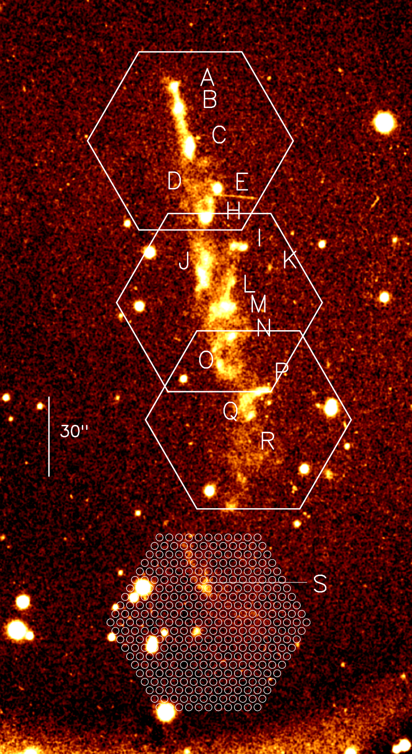
Figure 1: CCD image of HH 110 obtained at the Nordic Optical Telescope (NOT) through a narrow-band filter that includes the [S ii] 6716, 6731 Å lines (see López et al., 2005 for details). The four IFU pointing fields are superposed on the image. The knots discussed throughout this work are labeled on the image, according to the nomenclature first established by Reipurth & Olberg, 1991). The contours of the individual fibres have been drawn on the southern IFU field.

2 Observations and Data Reduction

Observations of HH 110 were made on 22 November 2004 with the 3.5-m telescope of the Calar Alto Observatory (CAHA). Data were acquired with the Integral Field Instrument Potsdam Multi-Aperture Spectrophotometer PMAS (Roth et al., 2005) using the PPAK configuration that has 331 science fibres, covering an hexagonal FOV of 74$\times$65 arcsec² with a spatial sampling of 2.7 arcsec per fibre, and 36 additional fibres to sample the sky (see Fig. 5 in Kelz et al. 2006). The I1200 grating was used, giving an effective sampling of 0.3 Å pix^-1 ($\sim 15$ km s^-1 for H$\alpha$) and covering the wavelength range $\sim 6500$–7000 Å, thus including characteristic HH emission lines in this wavelength range (H$\alpha$, [N ii] $\lambda\lambda$6548, 6584 Å  and [S ii]  $\lambda\lambda$6716, 6731 Å). The spectral resolution (i. e. instrumental profile) is $\sim 2$ Å  FWHM ($\sim 90$ km s^-1) and the accuracy in the determination of the position of the line centroid is $\sim 0.2$ Å  ($\sim 10$ km s^-1 for the strong observed emission lines). Four overlapped pointings were observed to obtain a mosaic of $\sim$ 5′$\times$ 1$\aas@@fstack{\prime}$5 to cover the entire emission from HH 110 (see Fig. 1). Table 1 lists the centre positions of each pointing, the exposure time and the HH 110 knots included in each pointing, following the nomenclature of Reipurth, Raga & Heathcote (1996).

Data reduction was performed using a preliminary version of the R3D software (Sánchez, 2006), in combination with IRAF and the Euro3D packages (Sánchez, 2004). The reduction consists of the standard steps for fibre-based integral field spectroscopy. A master bias frame was created by averaging all the bias frames observed during the night and subtracted from the science frames. The location of the spectra on the CCD was determined using a continuum-illuminated exposure taken before the science exposures. Each spectrum was extracted from the science frames by co-adding the flux within an aperture of 5 pixels along the cross-dispersion axis for each pixel in the dispersion axis, and stored in a row-stacked-spectrum (RSS) file (Sánchez, 2004). The wavelength calibration was performed by using the sky emission lines found in the observed wavelength range. The accuracy achieved for the wavelength calibration was better than $\sim 0.1$ Å ($\sim 5$ km s^-1). Furthermore, the large scale diffuse emission from this Orion region was subtracted from our data by using the signal acquired through the 36 additional sky fibres. Observations of a standard star were used to perform a relative flux calibration. The four IFU pointings were merged into a mosaic using our own routines, developed for this task (see e. g. Sánchez et al., 2007 and references therein). The procedure is based on the comparison and scaling of the relative intensity in a certain wavelength range for spatially coincident spectra. The pointing precision is better than 0.2 arcsec, according to the pointing accuracy of the telescope using the Guiding System of PMAS in relative offset mode (used for these observations). The overlap between adjacent pointings is $\sim$ 10–15% the field of view (more than 30 individual spectra). The merging process was checked to have little effect on the accuracy of the wavelength calibration of the final datacube making use of the sky lines (i. e. a common reference system) present in the spectra. A final datacube containing the 2D spatial plus the spectral information of HH 110 was then created from the 3D data by using Euro3D tasks to interpolate the data spatially until reaching a final grid of 2 arcsec of spatial sampling and with a spectral sampling of 0.3 Å . Further manipulation of this datacube, devoted to obtain integrated emission line maps, channel maps and position–velocity maps, were made using several common-users tasks of STARLINK, IRAF and GILDAS astronomical packages and IDA (García-Lorenzo, Acosta-Pulido & Megias-Fernández, 2002), a specific IDL software to analyse 3D data.

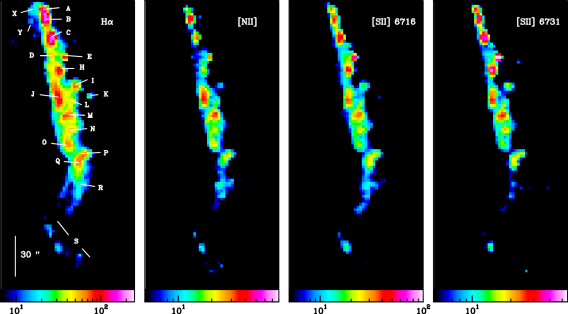
Figure 2: Integrated maps of the HH 110 emission obtained from the datacube by integrating the signal within the wavelength range including the line labeled in each panel: (H$\alpha$ : $\lambda$6558.3–6565.9 Å, [N ii] : $\lambda$6579.6–6585.8 Å, [S ii]  $\lambda$6716: 6712.8–6718.1 Å  and [S ii]  $\lambda$6731: 6727.2–6733.1 Å). Fluxes have been displayed in a logarithmic scale, in units of 10^-16 erg s^-1 cm^-2. In all the maps, north is up and East is to the left. The HH 110 knots and the spatial scale have been labeled in the H$\alpha$ panel (30 arcsec $\simeq$ 0.07 pc for a distance of 460 pc; Reipurth & Olberg, 1991).

Table 1: Positions of the single pointings of the HH 110 mosaic.

Position		Exp. time(s)	knot
05h51m25$\aas@@fstack{s}3$	+02$\degr$55$\arcmin$16$\arcsec$	1800	A-E
05h51m24$\aas@@fstack{s}4$	+02$\degr$54$\arcmin$20$\arcsec$	1800	I-N
05h51m23$\aas@@fstack{s}8$	+02$\degr$53$\arcmin$41$\arcsec$	2400	N-R
05h51m24$\aas@@fstack{s}9$	+02$\degr$52$\arcmin$40$\arcsec$	2700	S

3 Results

3.1 Physical conditions

3.1.1 Morphology

Some morphological differences have been found in previous narrow-band images of HH 110 between the H$\alpha$+[N ii] and [S ii] emissions. In an attempt to explore these differences, we obtained IFS-derived narrow-band images for each of the emission lines included in the observed spectral range (H$\alpha$, [N ii] $\lambda$ 6584 Å and [S ii] $\lambda$ 6716,6731 Å). For each position, the flux of the line was obtained by integrating the signal over the wavelength range of the line ($\lambda$ 6558.3–6565.9 Å for H$\alpha$; $\lambda$ 6579.6–6585.8 Å for [N ii]; $\lambda$ 6712.8–6718.1 Å for [S ii] $\lambda$6716 and $\lambda$ 6727.2–6733.1 Å for [S ii] $\lambda$6731), and subtracting a continuum, obtained from the adjacent wavelength range free of line emission. The narrow-band maps of HH 110 obtained from the IFS data (Fig. 2) are in good agreement with those obtained for this jet through ground-based, narrow-band images by different authors (see e. g. Reipurth, Raga & Heathcote, 1996; López et al., 2005). However, since the IFS data allow us to properly isolate the H$\alpha$ line emission from the [N ii] lines, we obtained the first known image of HH 110 in the [N ii] emission. In this sense, the IFS maps are better suited for comparing the jet morphology in the H$\alpha$ and [S ii] emissions, since the H$\alpha$ emission is not affected by the contamination from [N ii] lines.

Most of the HH 110 knots were detected in all the emission lines, although the brightness varies among different lines, being a signature of the excitation conditions, as we will discuss later. There are a few emission features whose brightness in the [N ii] and [S ii] lines should be very weak relative to the H$\alpha$ brightness and were barely detected or not detected at all in the [N ii] and [S ii] lines, namely: (i) the knot K, appearing quite isolated towards the western outflow edge, but outside the lower-brightness emission surrounding the knots, and (ii) the extended features towards the east of knots A to C, labeled X and Y. These faint H$\alpha$ features were first detected in the ground-based, narrow-band image of Reipurth & Olberg (1991). Our new IFS data indicate the X and Y features to be a ”true” emission in the H$\alpha$ line, having neither significant contributions from the extended nearby continuum (that was removed) nor from [N ii] lines (if any, it should be below the 3$\sigma$ rms level).

The knots are found surrounded by a lower-brightness nebular emission for all the emission lines. This more diffuse emission also shows a shock-excited spectrum, and likely arises from the gas in the boundary layer that is being incorporated into the outflow. The large scale, low-velocity diffuse emission component detected in the Orion region was removed from our data and is not contributing to this low-brightness, interknot emission structure we are referring to. Figure 2 shows that the cross section along all of the jet appears wider in H$\alpha$ than in the other lines, which all have similar spatial widths. Since with the present spatial resolution the sizes of the knots are similar at all lines, the wider H$\alpha$ cross-section of the jet should arise from the contribution of the low-brightness, nebular emission. In our maps, this weaker emission appears spatially more extended in H$\alpha$ than in the rest of the observed lines. This fact could be due, in part, to the weakness of the [N ii] and [S ii] emissions, which makes the emission undetectable in our maps (up to the 3$\sigma$ rms level) farther away from the knots.

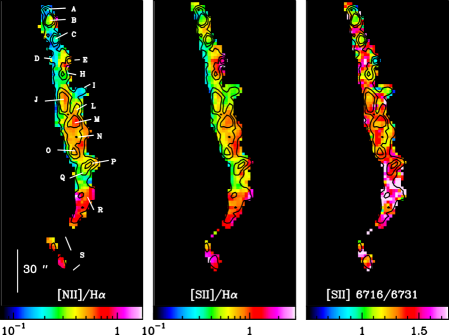
Figure 3: Line-ratio maps derived from the integrated line emissions displayed in Fig. 2. The [S ii]/H$\alpha$ and [N ii]/H$\alpha$ maps show the excitation conditions of the HH 110 emission, while the [S ii] 6716/6731 map traces the electron density. Contours of the integrated flux of the H$\alpha$ line have been overlaid to help with the knot identification, which have been labeled in the [N ii]/H$\alpha$ map.

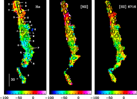
Figure 4: Flux-weighted mean velocity maps for the line labeled in the corresponding panel. Velocities (in km s^-1) are referred to the $V_{\mathrm{LSR}}$ of the parent cloud. Contours and knot identification, as in Fig. 3

3.1.2 Excitation and density conditions

First results on the physical conditions of HH 110 were obtained through long-slit spectroscopy acquired along the jet outflow (Reipurth, Raga & Heathcote, 1996; Riera et al, 2003a) and at a several positions across the jet beam (Riera et al, 2003a). The widths of the slits used in these observations were 2 and 1.5 arcsec, respectively. In both works, the [S ii]/H$\alpha$ ratios derived for the knots intersected by the slit along the jet axis outflow range from $\sim$0.2 to $\sim$0.7. These ratios correspond to an intermediate/high degree of excitation (Raga et al., 1996). A trend was found of an increasing [S ii]/H$\alpha$ ratio (hence a decrease of the excitation) moving from knot C to knot M, where the lowest excitation was detected. A decrease of this ratio (hence an increase of the excitation) was found beyond knot M. In general, the values derived in both works are well consistent, except for knots A and N, where the [S ii]/H$\alpha$ ratio reported by Riera et al (2003a) is significantly higher (by a factor of two) than the ratio reported by Reipurth, Raga & Heathcote (1996). This is not surprising since the excitation conditions should change significantly within arcsecs across the jet beam, as first revealed by the spectroscopy of the jet cross section performed by Riera et al (2003a). Thus, the sampled regions of knots A and N might not coincide in both observations. Furthermore, no clear trends for the excitation structure of the jet cross sections were found from the spectra acquired by Riera et al (2003a). These authors found a complex structure at the four positions across the jet beam, where the spectra were obtained.

To look for a more complete picture of the entire spatial structure of the excitation and density of the jet, we obtained the [S ii](6716+6731)/H$\alpha$ and [N ii](6548+6584)/H$\alpha$ line-ratio maps from the IFU data (Fig. 3). The line-ratio maps were created by dividing spaxel-by-spaxel the corresponding flux-integrated line maps (all the spaxels with values below 5$\sigma$ were blanked before to obtain the line-ratio map). At the weakest knots, the estimated uncertainties are 10% and 15% in the [S ii](6716+6731)/H$\alpha$ and [N ii](6548+6584)/H$\alpha$ line-ratio values respectively.

The [S ii]/H$\alpha$ and [N ii]/H$\alpha$ maps clearly reveal the complex excitation structure of the emission that was only barely outlined from long-slit spectroscopy. Several facts should be remarked: (i) for the knots that were sampled through long-slit spectroscopy, the line-ratio values derived from the IFS data around the peak positions are in good agreement with those derived from the long-slit spectra. For knots A and N, the ratios obtained from the IFS data are in better agreement with those derived by Riera et al (2003a) than with those derived by Reipurth, Raga & Heathcote (1996); (ii) IFS line-ratio maps revealed some regions in which the degree of gas excitation is low. In particular, the highest [S ii]/H$\alpha$ ratios ($\geq$ 1.5) are found around knot H and slightly lower ratios, which are also compatible with a low degree of excitation, are found around knots R and S. This wider range of excitation degree could not be detected by previous long-slit observations, which did not sample these low excitation regions; (iii) no clear systematic trend in the spatial distribution of the excitation was found neither along the jet outflow nor across the jet beam. However, the integrated [S ii]/H$\alpha$ and [N ii]/H$\alpha$ maps indicate that the excitation is higher for the northern jet knots A to D (where the outflow has a higher collimation) than beyond knot E, from the region where the outflow widens and the knots begin to lose their alignment relative to the axis direction traced by knots A-C. For this jet region (i. e. from knots E to Q) the line ratio maps show some signatures of an increment in the excitation moving outwards, from the knot peak to the eastern knot border and to the interknot. The line ratio maps are thus suggestive of a decrease in the excitation from east to west across the jet beam. This is true for all knots, except around knot I (at the western jet border), where the excitation is higher and similar to that derived in the northern (A to D) knots.

The spatial distribution of the electron density ($n_{\mathrm{e}}$) is traced by the [S ii] 6716/6731 map. Figure 3 shows the map created from the IFU data (with the assumptions mentioned before for the excitation maps). At the weakest knots, the estimated uncertainty is 15%. The values found range from $\sim$ 0.9 to $\sim$ 1.4, which correspond to $n_{\mathrm{e}}$ ranging from 1000 to 50 cm^-3 respectively (these values were derived using the TEMDEN task of the IRAF/STSDAS package, and assuming $T_{\mathrm{e}}=10^{4}$ K). The electron density cannot be properly evaluated around the knot R region, because the derived line ratios are higher than the values for which the [S ii] 6716/6731 is density sensitive in the low-density limit. In general, the trend found is a decrease in the $n_{\mathrm{e}}$, moving along the jet from north to south. This result is consistent with the density behaviour of the knots derived from the long-slit spectra by Reipurth, Raga & Heathcote (1996) and Riera et al (2003a). However, the spatial distribution of the density obtained through IFS (Fig. 3) is more complex than that outlined from long-slit spectroscopy, and could not be properly described based on this kind of observations. The density map indicates that, in general, the electron densities are higher around the knot peak positions and decrease towards the edges of the knots and towards the interknot gas. Across the jet beam, a trend is observed in the knots peaking towards the west side of the axis defined by knots A–C (e. g. knots E, I, N, P) that are denser than knots peaking towards the east side of this axis (e. g. knots D, J, O, Q). The density map also shows some local departures of this general trend that are significant. In particular, it should be noted that the highest $n_{\mathrm{e}}$ is reached around knot E (i. e. $\sim$ 40 arcsec south from knot A). In fact, the IFU data revealed an enhancement in the electron density, reaching $n_{\mathrm{e}}$ values of $\simeq$ 1000 cm^-3 and with a maximum of $\simeq$ 1300 cm^-3 located $\simeq$ 3 arcsec southwest of the knot E peak intensity. This denser clump, extending over $\simeq$ 30 arcsec², appears well delimited at its eastern edge, as shown by a sharp fall of $n_{\mathrm{e}}$, which reaches values of $\simeq$ 200–300 cm^-3 by only moving $\simeq$ 2 arcsec east from the E peak intensity. In addition, although $n_{\mathrm{e}}$ gently decreases from knots A ($\sim$ 600 cm^-3) to H ($\sim$ 400 cm^-3), the knot I, southwest of all of these knots, has a $n_{\mathrm{e}}$ similar to knot B ($\sim$ 500 cm^-3), while knot D, southeast of knot C, has similar low values ($\sim$ 150 cm^-3) to those found at the southern, more rarefied knots, beyond knot N.

3.2 Kinematic analysis

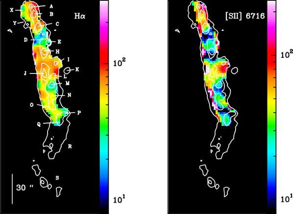
Figure 5: Maps of the FWHM (in km s^-1) for the line labeled in the corresponding panel. Contours and knot identification, as in Fig. 3. Spaxels with a FHWM below 115 km s^-1have been blanked. (At several positions, like in the southern knots, FWHM should be narrower and could not be properly determined due to the instrumental line profile).

3.2.1 Spatial velocity distribution

The emission lines at most of the positions mapped in HH 110 show asymmetric profiles that cannot be properly fitted by a single Gaussian. Hence, we calculated the flux-weighted mean radial velocity (or first-order intensity momentum) instead of the line centroids of a Gaussian fit, and the flux-weighted rms width of the line (or second-order intensity momentum), proportional to the FWHM of the line, and described the integrated velocity field of the jet from these intensity momenta. HH 110 shows a velocity field behaviour very similar in all the mapped lines (Fig. 4). The radial velocities are blueshifted ($V_{\mathrm{LSR}}$ ranging from $\sim$ –10 to –80 km s^-1 in H$\alpha$), with an increase towards more blueshifted values moving from north to south. Velocities that were derived from H$\alpha$ are blueshifted by $\sim$ 20 km s^-1relative to those derived from the [N ii] and [S ii] (the velocities derived from these two lines are similar). The velocity offset found between H$\alpha$ and [S ii] is not an artifact caused by an inaccurate wavelength calibration of the IFS data, since it has been also found in long-slit, higher resolution data (e. g. López et al., 2005). A more detailed inspection of the velocity maps reveals a more complex structure of the velocity field: (i) the less blueshifted velocities ($V_{\mathrm{LSR}}$ $\sim$ –10 to –15 km s^-1 in H$\alpha$) are found around the northern emissions X, Y and in knot D, all of them located towards the eastern side of the jet axis direction traced by the knots A–C; (ii) conversely, more blueshifted velocities ($V_{\mathrm{LSR}}$ $\sim$ –50 to –60 km s^-1 in H$\alpha$) appear around the regions of knot O and Q, which also are located at the eastern jet side. Even more blueshifted velocities (up to $V_{\mathrm{LSR}}$ $\sim$ –80 km s^-1 in H$\alpha$) are found around knots I and K, located at the western jet border, quite outside of the main jet body.

The maps of the FWHM for the H$\alpha$ and [S ii] $\lambda$ 6716 Å lines obtained from the second-order intensity momentum are shown in Fig. 5. Maps were corrected from the instrumental profile by subtracting it in quadrature spaxel-by-spaxel. Spaxels with values below a 5$\sigma$ rms level were blanked. The spatial distribution of the FWHM shows a complex pattern in both lines. In general, widths are broader for H$\alpha$ than for the [S ii] lines. The FWHM of the H$\alpha$ ranges from 30 to 90 km s^-1, being in good agreement with those found by Riera et al (2003b) from Fabry-Perot data and with those derived by Hartigan et al. (2009) from long-slit, high-resolution spectra. The northern knots (A to C) present the largest values (80–90 km s^-1) of the FWHM, decreasing towards the south of the outflow (up to 30–40 km s^-1 around knots M and Q). In fact, the FWHM around the arc-shaped, southern S emission region should be even narrower, but the widths could not be properly evaluated due to the instrumental line profile. Like for other jet properties, this general trend is not well fulfilled by the whole outflow: a region having significant narrow lines, their widths being close to detection limit, is also found around knot D, while higher FWHM values (90 km s^-1, similar to the widths derived around knot A) are found around knot I. Concerning the FWHM of the [S ii] lines, their values range from 20 to 70 km s^-1and are in agreement with the results of Hartigan et al., 2009). The spatial distribution of the FWHM values for the [S ii] lines are similar to the FWHM H$\alpha$ map. Some key differences in FWHM between H$\alpha$ and [S ii] should be mentioned: (i) the widths of the [S ii] lines drop significantly around knot C, where its value diminished by a factor of two relative to that found around knot A, while knots C and A have comparable FWHMs in H$\alpha$; (ii) knots M and Q have very similar FWHM values in [S ii] and H$\alpha$, while the general trend for the rest of the knots is the H$\alpha$ line being wider (by 15–20 km s^-1typically) than the [S ii] line.

3.2.2 Peak intensity knot velocities

In an attempt to compare long-slit and IFS data, we have obtained a representative spectrum for each jet knot by extracting the spectrum of the spaxel (aperture of 2 arcsec) that corresponds to the position of the knot intensity peak (Fig. 6). The knots show significant differences in their physical conditions, as inferred from their relative line intensities. Moreover, the lines present asymmetric profiles that in some knots are suggestive of being double-peaked (see, e. g. knots H, I) although the profiles cannot be resolved because of the spectral resolution of the data.

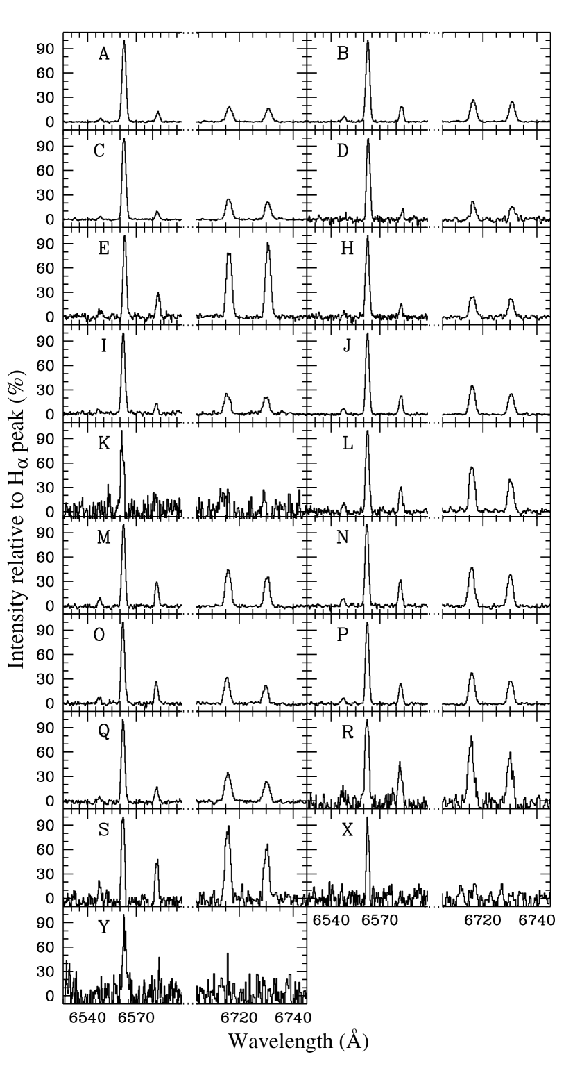
Figure 6: Spectra of the HH 110 knots in the spectral windows including H$\alpha$ + [N ii] and [S ii] 6716, 6731 lines. Each spectrum has been extracted for the spaxel that corresponds to the peak intensity position (i. e.within an aperture of 2 arcsec) and its intensity has been normalized to the H$\alpha$ peak intensity.

Figure 7 displays the radial velocities at the position of the knot peak intensity, in both H$\alpha$ and [S ii] lines, as a function of the distance to knot A. The two radial velocity fields are very similar. A trend of increasing blueshifted (more negative) velocity values with the distance to knot A is outlined. This trend is consistent with the velocity behaviour found in previous works (Riera et al, 2003b; Hartigan et al., 2009). The radial velocities of some knots present deviations of this general trend. In particular, the isolated knot K (found outside the jet body) has a blueshifted radial velocity more negative than the rest of the knots, and its deviation from the general trend is statistically significant. A linear fit of the peak radial velocity of the H$\alpha$ line with distance, including all the knots (19), was obtained (correlation coefficient $r=0.61$; rms fit residual $\sigma=15.1$ km s^-1). The fit is shown in Fig. 7 by a continuous straight line, and the $1\sigma$ deviation from the fit, by the dashed lines. Knot K deviates from the fit by $3\sigma$. This deviation is statistically significant for a sample of 19 knots. Then, a new linear fit was calculated after removing knot K from the sample (i.e. 18 knots). We obtained values of $r=0.74$ and $\sigma=10.5$ km s^-1. The knots that deviate more than $1.5\sigma$ from this new fit are knot O ($1.8\sigma$ deviation), I ($2.2\sigma$ deviation), and K shows now a $4.6\sigma$ deviation. Unfortunately there is no proper motion determination for knot K that would allow us to calculate the projection angle of its motion. Hence, the current data do not allow us to discern whether the kinematic behaviour of knot K, with a radial velocity appreciably blueshifted as compared with the rest of the knots, can be only attributed to the jet geometry (i.e. to projection effects). Recently, Hartigan et al. (2009) imaged the HH 110 region in the H₂ 2.12 $\mu$m line. They report a weak jet emerging from the source IRS1 (to the west of HH 110) and extending from north to south. This weak jet seems to be pointing at knot K. In conclusion, there are some indications (a location isolated from the jet flow, and a kinematics significantly different from the rest of the knots) that knot K could be related to IRS1, but its relationship with the HH 110 outflow cannot be fully discarded based on the results presented in this work.

The full spatial velocity ($V_{\mathrm{tot}}$) and an upper limit for the angle $\phi$ between the knot motion and the plane of sky ($\phi$=0^∘ when the flow moves in the plane of the sky) were calculated from the knot proper motions, derived from multiepoch [S ii] narrow-band images (López et al., 2005) and the radial velocities, derived in this work from the [S ii] lines at the position of the knot intensity peak (the typical errors for $\phi$ and $V_{\mathrm{tot}}$  are $\sim$ 6^∘ and $\sim$ 12 km s^-1 respectively). The results are displayed in Fig. 8.

The values derived for the inclination angle suggest that the flow remains close to the plane of the sky ($\phi~{}\leq$ 20^∘ for most of the knots). The inclination gently increases from $\phi~{}\simeq$ 8^∘ at the beginning of the outflow (around knot A) to higher values ($\geq$ 30^∘) for distances $\geq$ 150 arcsec from knot A (around knots R and S, coinciding with the region where the outflow has a highly curved shape).

As can be seen from Fig. 8 (lower panel), the spatial velocity ($V_{\mathrm{tot}}$) derived at most knots is $\geq$ 100 km s^-1. There is a trend of decreasing velocity with distance along the outflow, from $V_{\mathrm{tot}}$ $\simeq$ 185 km s^-1 for knot A to $V_{\mathrm{tot}}$ $\simeq$ 75 km s^-1 for knot S. A few knots present a deviation from this velocity trend that might be significant: knot O, with a higher velocity ($V_{\mathrm{tot}}$$\simeq$ 190 km s^-1) than the neighbouring knots ($V_{\mathrm{tot}}$$\leq$ 150 km s^-1), and knots E and B, having lower $V_{\mathrm{tot}}$ than the neighbouring knots. In particular, the lowest spatial velocity is obtained at knot B ($V_{\mathrm{tot}}$$\simeq$ 25 km s^-1). This value is far from the spatial velocities of its neighbouring knots ($V_{\mathrm{tot}}$$\geq$ 165 km s^-1) and even far from the velocities of the slower knots. In order to better visualize the velocity behaviour to we are referring, a linear fit was calculated after removing knot B from the sample (i. e. 14 knots). The fit (correlation coefficient $r=0.53$; rms fit residual $\sigma$=31.8 km s^-1) has been drawn in Fig. 8 by a continuous straight line, and the 1$\sigma$ deviation from the fit, by the dashed lines. As can be seen from the figure, the spatial velocity deviates $\leq$ 1$\sigma$ for most of the knots. A few knots lie outside the region delimited by the dashed lines: knot O (2.2$\sigma$ deviation above the fit), knot E (2.3$\sigma$ below the fit) and knot B (4.3$\sigma$ below the fit). The region around knot B could correspond to the region where the outflow is excavating a channel through the dense molecular clump (Reipurth, Raga & Heathcote, 1996; López et al., 2005) and might trace the location where the jet collides with the cloud. Hence, significant deviations from the kinematics trend that account for the jet/cloud interaction should be expected at this location. This may explain the appreciably low spatial velocity found for knot B. Concerning the other two knots with deviations less significant, knot O also has a highly blueshifted radial velocity, (although within a 1$\sigma$ deviation from the radial velocity fit, see Fig. 7). The low $V_{\mathrm{tot}}$ at knot E mostly corresponds to the tangential velocity component (see also Fig. 7) As was mentioned before, the highest values of the electron density in the outflow, measured from the integrated [S ii] line ratio, are found around knot E location. Thus, similarly to what happens around knot B, a stronger interaction between the jet and the inhomogeneous ambient material around the knot E location might be producing these departures in the kinematics and physical conditions relative to those found at the surrounding knots.

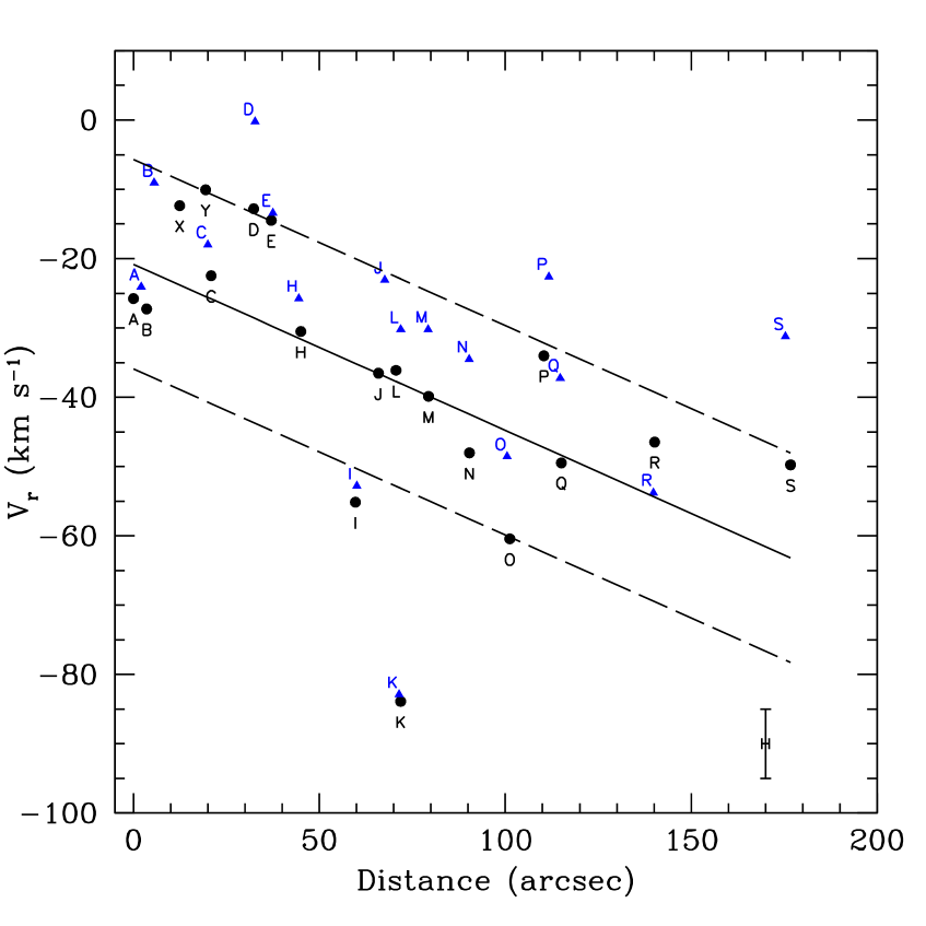
Figure 7: Radial velocities measured at the position of the peak intensity of the HH 110 knots, as a function of distance to the knot A peak intensity in H$\alpha$. The black dots correspond to the values derived from H$\alpha$ and the blue triangles, from the [S ii] lines. The typical value of the velocity error is $\sim$ 10 km s^-1and the uncertainty in the knot position $\sim$ 1 arcsec, and are displayed in the lower-right corner of the figure. The straight lines mark the linear fit to the data (solid line) and the 1 $\sigma$ deviation from the fit (dashed lines).

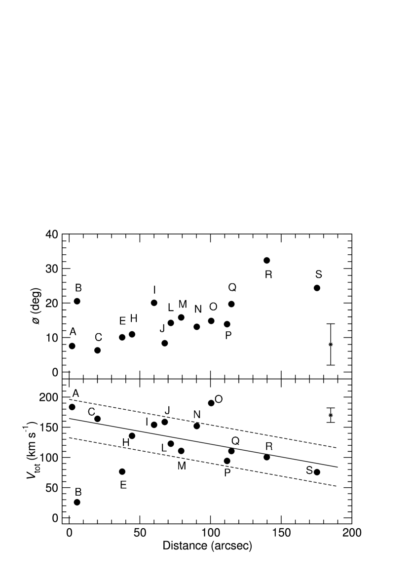
Figure 8: Total velocities (lower panel) and inclination angle, defined by the direction of the knot motion and the plane of the sky (upper panel) as a function of distance to the position of the [S ii] intensity peak of knot A. The typical values of $\phi$ and $V_{\mathrm{tot}}$ errors are $\sim$ 6^∘ and $\sim$ 12 km s^-1, respectively and are displayed at the corner of each panel. The uncertainty in the knot position ($\sim$ 1 arcsec) is smaller than the size of the symbols. Straight lines that mark the linear fit to the data (solid line) and the 1 $\sigma$ deviation from the fit (dashed lines) are drawn on the velocity panel.

3.2.3 Line Profile Shapes

As already mentioned in §3.2.1, the line profiles show some degree of asymmetry relative to a single-Gaussian shape that varies from knot to knot. This can be seen for the H$\alpha$ and [S ii]  lines of the spectra extracted at the position of the peak intensity of each knot (Fig. 6). The analysis of spectral line asymmetries through line bisectors provides a strong tool to understand the shape and origin of line profiles, and is widely used in stellar astrophysics (see e. g. Queloz et al., 2001; Dall et al., 2006; Martínez-Fiorenzano, 2008). In order to make more clear the asymmetries of the HH 110 line profiles, we calculated the line bisectors for the H$\alpha$ line at the position of the knot peak intensity. The results are shown for each profile in Fig. 9. We found knots with some high-velocity emission excess, as shown by the tilt of the line bisector towards blueshifted wavelengths (knots A, C, D, H, J, L, M, O, P, R and S). We will refer to these knots as those having ”blue asymmetry”. For other knots, there is low-velocity emission excess, with the line bisector tilted towards redshifted wavelengths (referred as knots having ”red asymmetry”: knots E, I and Q). Finally, a few knots show a nearly symmetric profile (knots B and N). Such line-profile behaviour might be explained in part by the combined effect of the knot velocity and flow inclination at the knot position.

Some clues can be obtained from the work of Hartigan, Raymond & Hartmann (1987), who modeled the effect of varying the velocity and the inclination angle of the flow in the plane of the sky on the H$\alpha$ line profiles emerging from bow shocks. They found that the asymmetry of the line profile increases with the velocity of the shock, and with the inclination angle. Resolved, double-peaked profiles are only found for velocities higher than $\simeq~{}150$ km s^-1and for angles greater than $\simeq~{}45^{\circ}$. Furthermore, moderate variations on the inclination angle result in significant effect in the shape of the line profile. For a given angle, the shape of the asymmetry changes from ”red” to ”blue” depending on the velocity: e. g. for low inclination angles ($\leq~{}30~{}^{\circ}$), a ”red asymmetry” is obtained for low velocities ($\leq 100$ km s^-1) and a ”blue asymmetry” for higher velocities ($\simeq 200$ km s^-1).

Interestingly, most of the HH 110 knots showing a ”blue asymmetry” in the line profile correspond to knots having high velocity ($V_{\mathrm{tot}}$ $\geq$ 160 km s^-1, e. g.: A, C, J, O) or inclination angle $\phi~{}\simeq~{}30^{\circ}$ (e. g.: R, S). ”Red asymmetry” is observed in knots with lower velocities (e. g.  E, with $V_{\mathrm{tot}}$ = 80 km s^-1and Q, with $V_{\mathrm{tot}}$ = 110 km s^-1) and lower inclination angles ($\phi~{}\leq~{}20^{\circ}$). Note in addition that some pairs of knots with close values of $V_{\mathrm{tot}}$ and $\phi$ show very similar profiles, as is the case of knots C and J, and of knots H and L.

Hence, there is a general agreement of the H$\alpha$ line profiles observed in HH 110 with the obtained from the shock models of Hartigan, Raymond & Hartmann (1987). However, other properties of the emission could also being contributing to the line shapes. For example, different morphologies of the bow emission, keeping all the other parameters constant, can give different line profiles, as shown by Schultz, Burton & Brand (2005). They found that the bluntness at the apex and the radius of the tail are two important factors in determining the line profiles for the case of H₂ lines arising from a bow-shock. In fact, Hartigan et al. (2009) found from laboratory jet experiments how the working surface of a deflected bow shock present complex emission structures as those observed in HH 110. These structures give rise to different asymmetric line profiles, depending on the HH 110 knot and hence, on the shock velocity and projection angle.

Figure 9: H$\alpha$ line profiles of the knots labeled in each panel, obtained from the spectra extracted at the position of the knot peak intensity (see Fig. 6). The line bisector has been drawn for each profile. In each panel, the line intensity has been normalized to the value at the peak. On the x-axis, the wavelengths are relative to the rest H$\alpha$ wavelenght.

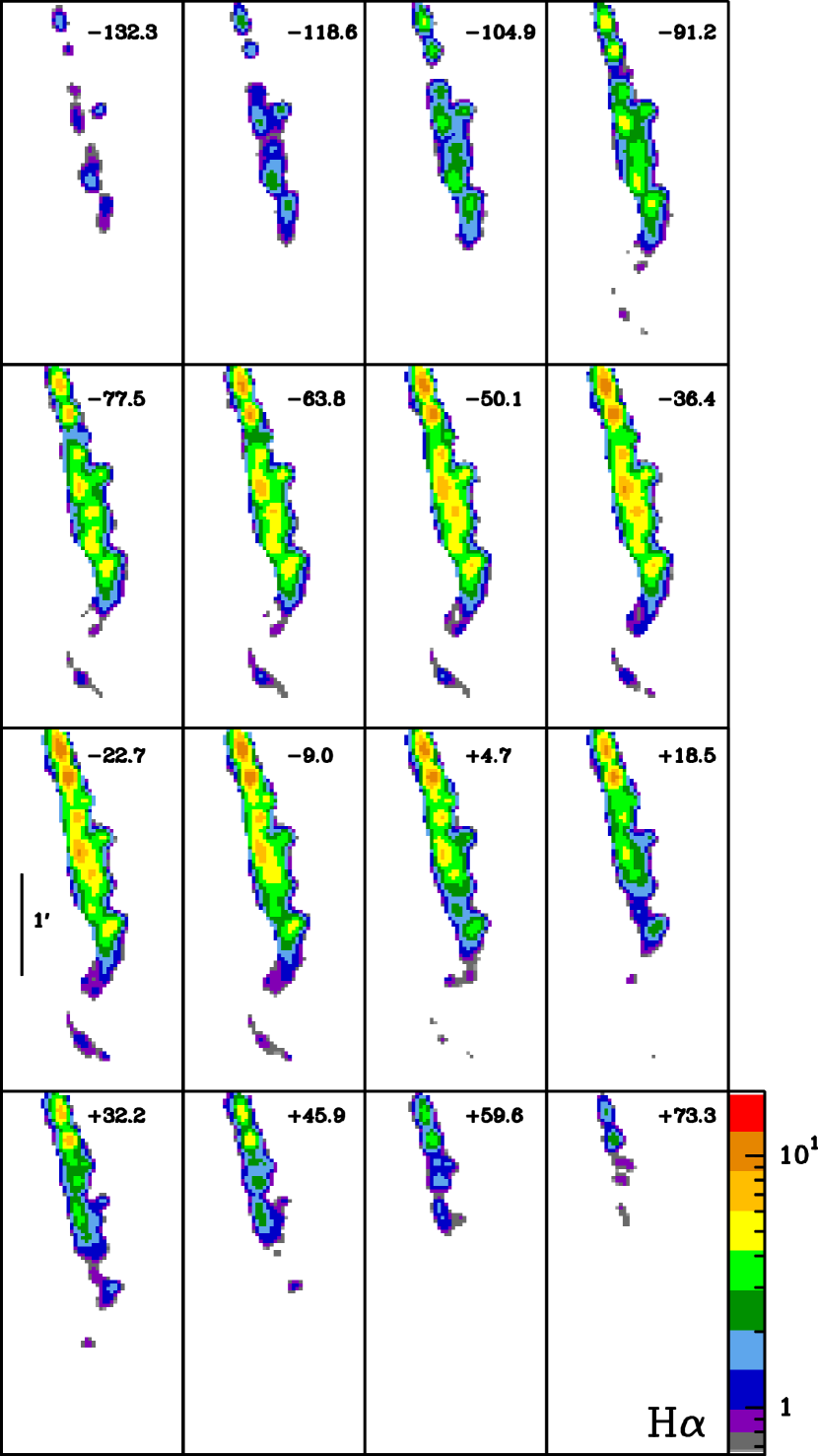
Figure 10: H$\alpha$ channel maps centred on the $V_{\mathrm{LSR}}$  radial velocities (km s^-1) labeled in each panel. The spatial scale is given in one of the panels. Fluxes have been displayed in a logarithmic scale, in units of $10^{-16}$ erg s^-1 cm^-2.

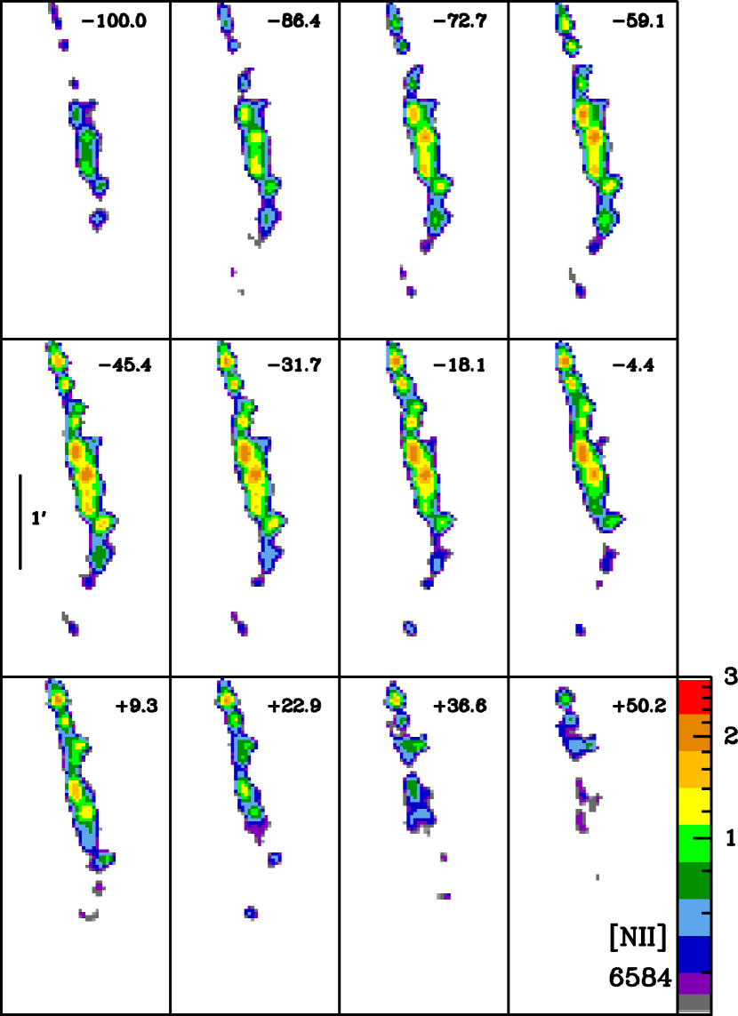
Figure 11: Same as Fig. 10, but for the [N ii] 6584 Å  emission line.

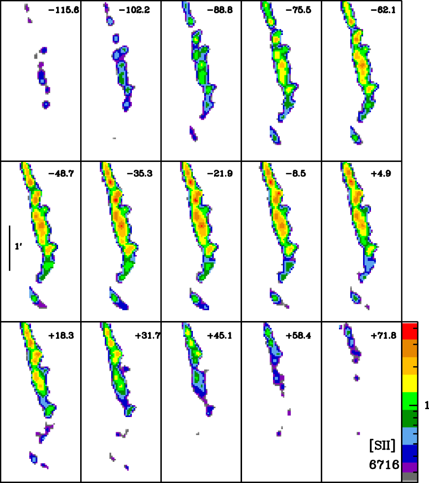
Figure 12: Same as Fig. 10, but for the [S ii] 6716 Å  emission line.

3.2.4 Kinematics behaviour of physical conditions: channel maps

A more detailed sampling of the gas kinematics was obtained by slicing the datacube into a set of velocity channels. Each slice corresponds to a constant wavelength bin of 0.3 Å (i. e. a velocity bin of $\sim~{}$14 km s^-1: 13.7 km s^-1 for H$\alpha$ and [N ii], and 13.4 km s^-1 for [S ii]). Hence, we have obtained the channel maps for each of the emission lines within the observed wavelength range, namely H$\alpha$, [N ii] $\lambda$ 6584 Å and [S ii] $\lambda$ 6716 Å , as illustrated in Figs.   10, 11 and 12, respectively. Moreover, we also analysed the behaviour of the excitation and density as a function of the velocity.

The emission detected above a 3$\sigma$ SNR level spreads over different velocity ranges, depending on the line. Emission in H$\alpha$ was detected over a wider velocity range ($\simeq$ 200 km s^-1, from –135 to +75 km s^-1) than in [S ii] ($\simeq$ 180 km s^-1, from –115 to +70 km s^-1) and in [N ii] ($\simeq$ 150 km s^-1, from –100 to +50 km s^-1). Note, however that the morphology of the emission does not significantly differ among the three lines when channels of similar velocities are compared.

H$\alpha$ emission covering the whole velocity range was only detected at the northern, more collimated flow region, from knots A to H. For velocities ranging from $\simeq$ –80 to –10 km s^-1, there is emission detection from all the knots, the stronger emission coming from the $\simeq$ –50 to –23 km s^-1channels. Emission from velocities more blueshifted than $\simeq$ –90 km s^-1or more redshifted than $\simeq$ +20 km s^-1were not detected (up to a 3$\sigma$ snr level) beyond knot Q, from the loci where the flow trajectory appreciably changes its path. The kinematic behavior in the [N ii] emission is similar to that found in H$\alpha$, although the velocity range with emission detection is different. In this sense, the [N ii] emission arising from most of the knots covers a range from $\simeq$ –60 to +10 km s^-1, the stronger emission coming from the $\simeq$ –45 to –18 km s^-1channels. [N ii] emission was not detected from the southern knots, beyond knot Q, with the exception of some hint ($\leq 2\sigma$ snr level) at $\simeq$ –18 km s^-1around knot R. Note in addition the lack of [N ii]  emission from knots A to C for velocities more blueshifted than $\simeq$ –90 km s^-1. Finally, we detected [S ii] emission from the whole flow covering a range from $\simeq$ –90 to +18 km s^-1, the stronger emission coming from the $\simeq$ –35 to –8 km s^-1channels. As in the case of H$\alpha$ and [N ii] , there are neither emission more blueshifted than $\simeq$ –90 km s^-1nor more redshifted than $\simeq$ +20 km s^-1detected beyond knot Q.

Line-ratio channel maps were created from the IFU data (as mentioned in §3.1.2 for the integrated line-ratio maps) to analyse the excitation and density as a function of the velocity. The estimated uncertainties are better than 25% in the [N ii]6584/H$\alpha$ and 10–15% in the [S ii](6716+6731)/H$\alpha$ and [S ii] 6716/6731 maps. Figures 13 and 14 display the [S ii](6716+6731)/H$\alpha$ and [N ii]6584/H$\alpha$ line-ratio channel maps, tracing the gas excitation as a function of the radial velocity.

The line-ratio maps for each velocity channel follow the spatial behaviour of the excitation that was already found in the integrated line-ratio maps (Fig. 3). The gas excitation is higher (i. e. lower [S ii]/H$\alpha$ line-ratio values) at the northern knots (A–D), and becomes lower (i. e. the [S ii]/H$\alpha$ line-ratio values increase) beyond knot E, along the region where the flow cross section widens. Furthermore, the trend found for this region (a decreasing excitation moving across the jet beam, from the eastern jet side to the west) is now more clearly seen on each of the channel map. An opposite trend of increasing excitation from east to west is outlined at the curved, terminal S region from the –45 km s^-1 $<$$V_{\mathrm{LSR}}$$<$+5 km s^-1channels, where the signal is large enough to evaluate the ratio with confidence.

In addition, the line-ratio channel maps indicate that the gas excitation varies depending on the gas kinematics, namely higher excitation (i. e. lower [S ii]/H$\alpha$ line ratios) for the higher velocities (in absolute value, both blueshifted and redshifted) and lower excitation (higher line ratios) for lower (in absolute value) velocities. The differences are found for most of the knots. For example, for knot C, at the position of its peak intensity, we measured a [S ii]/H$\alpha$ ratio $\leq$ 0.2 for $V_{\mathrm{LSR}}$ $\leq$ –90 km s^-1 and $V_{\mathrm{LSR}}$ $\geq$ +30 km s^-1, while a ratio of $\geq$ 0.5 is found for –50 km s^-1 $<$ $V_{\mathrm{LSR}}$ $<$ +20 km s^-1. The same behaviour appears for low-excited knots: at the peak intensity position of knot M, the [S ii]/H$\alpha$ ratio is $\geq$ 1.1 for –30 km s^-1 $<$ $V_{\mathrm{LSR}}$ $<$ +20 km s^-1, being $\leq$ 0.5 for $V_{\mathrm{LSR}}$ $\leq$ –90 km s^-1 and $V_{\mathrm{LSR}}$ $\geq$ +30 km s^-1.

The [S ii] 6716/6730 line-ratio channel maps (Fig. 15) trace the electron density of the emitting gas as a function of the radial velocity. In general, the spatial distribution of the density follows the same trends that were found from the integrated [S ii] 6716/6730 line-ratio (Fig. 3). In this sense, density decreases from north to south along the jet, but with some exception, e. g. around knot E, where density is the largest. Variations on the electron density also depend on the gas kinematics. For a given knot, the largest electron density corresponds to the emission moving at lower (in absolute value) velocities (typically within the range –25 km s^-1$<$$V_{\mathrm{LSR}}$$<$+5 km s^-1), whereas the density falls down to $\simeq$ 40–50% for the emission moving at high velocity ($V_{\mathrm{LSR}}$$\geq$ +20 km s^-1and $V_{\mathrm{LSR}}$$\leq$ –60 km s^-1). Hence, the emission from slower gas appears denser and less excited than the faster (red or blueshifted) emission, which is more excited and rarefied.

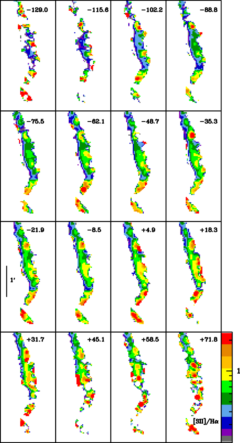
Figure 13: The [S ii]/H$\alpha$ line-ration maps, tracing the gas excitation, derived from the channel maps at the $V_{\mathrm{LSR}}$ labeled in the corresponding panel.

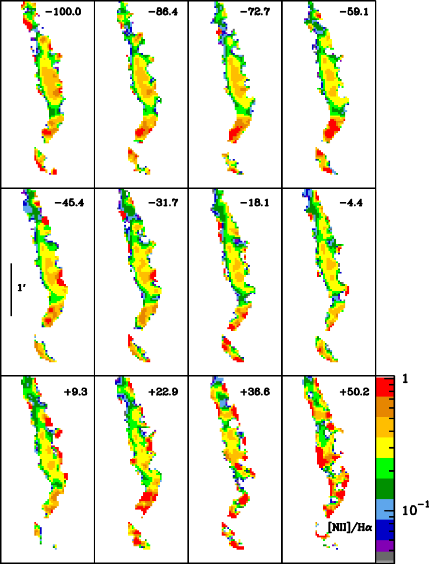
Figure 14: Same as Fig. 13, but for the [N ii]/H$\alpha$ line-ration maps.

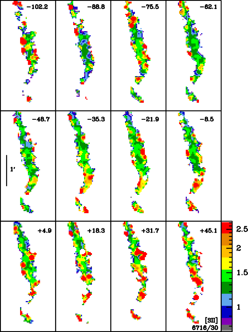
Figure 15: The [S ii]6716/6731 line-ratio maps, tracing the electron density, derived from the channel maps at the $V_{\mathrm{LSR}}$ labeled in the corresponding panel.

4 Summary and Conclusions

To conclude, the IFS data confirm the peculiar nature of HH 110 as compared with most of the stellar jets already observed. The most relevant results presented in this paper might be summarized as follows:

• These IFS data have allowed us to generate the first [N ii] narrow-band image of HH 110 currently obtained, which shows a similar jet cross section to the [S ii] emission. In addition, these data allow us to confirm that the faint filamentary emission labeled X and Y, detected to the east of knots A–C, which probably corresponds to a ”fossil” outflow channel, mainly should arise from ”true” H$\alpha$ line emission. The contributions from nearby continuum or from the [N ii] lines, if any, should be very weak, as no emission was detected in [N ii], and the continuum contribution was previously removed.

• The line-ratio maps derived from the integrated line intensities revealed complex spatial structures for the gas excitation and electron density. Although the line ratios that trace gas excitation are indicative of an intermediate/high-excitation degree for most of the emission mapped, several regions of low-excitation emission are detected through the flow (e. g. [S ii]/H$\alpha$ $\geq$ 1.5 around knot H). In general, the [S ii] line ratios correspond to low electron density values ($n_{\mathrm{e}}$ $\leq$ 1000 cm^-3) and show smooth spatial variations. However, strong local enhancements of $n_{\mathrm{e}}$ relative to its surroundings were detected at several locations (e. g. around knot E, where the $n_{\mathrm{e}}$ value is about three times that of the surroundings).

• Radial velocities appear blueshifted, relative to the $V_{\mathrm{LSR}}$ of the cloud, the modulus increasing with the distance to knot A, although with some appreciable local departures from this trend (in particular, knot K). This systematic increase in radial velocity should not be interpreted as a sign of jet acceleration, since no similar trend was derived for proper motions. In fact, the trend found for tangential velocities goes in the opposite way (decreasing velocity as a function of distance from knot A, with some appreciable local departures, e. g. in knot B). Thus, this apparent acceleration should be better attributed to a geometric effect: the interaction between the jet and the inhomogeneous ambient surroundings will lead to the deflection of the jet and therefore, to changes in the projection of the full spatial velocity along the line of sight (radial velocity) and along the plane of the sky (tangential velocity).

• In general, the line profiles are broader for H$\alpha$ than for [S ii], and the FWHM in both lines decreases from the northern to the southern knots, although this trend is not fully systematic along the outflow.

• We recalculated the full velocity and the motion direction relative to the plain of sky of the HH 110 knots using the [S ii] radial velocities, derived from the spectra extracted at the position of the knots peak intensity, together with knot proper motions, obtained from ground-based, multi-epoch [S ii] narrow-band images. We confirmed the general trend of a decrease in the velocity and an increment in the projection angle with distance from knot A, as found in previous works that used a more limited knot sample. Significant departures from the trend are found in some knots. These knots could be tracing the loci where a stronger interaction between the jet and the inhomogeneous medium is taking place.

• The channel maps showed that the emission spreads over different velocity ranges, depending on the line considered. In spite of that, the maps also showed that the morphology of the emission in each of the velocity channels is similar for all the lines, the strongest emission corresponds to the velocity interval $\simeq$–20$<$$V_{\mathrm{LSR}}$$<$+5 km s^-1, where significant emission from all the knots was detected. In addition, the previously unknown kinematics of the excitation and electron density along the full spatial extent of the outflow were obtained from the channel maps. The degree of excitation and the electron density appear to be anticorrelated with the velocity modulus, in the way that the emission from the gas moving faster (either, at red or blueshifted velocities) has higher excitation and lower density as compared to the emission from the gas moving at slower velocities, which appear denser and less excited.

• From the IFS spectra extracted at appropriate spaxels, we were able to compare the physical conditions obtained from these data with those derived from previous long-slit and Fabry-Perot observations. The general trends followed by the properties of the emission and even the derived values of the observables are in good agreement at all the commonly sampled positions. However, the complex structure of the HH 110 kinematics and physical conditions, already outlined in previous works, has been now better characterized from this more complete IFS sampling. These data revealed significant variations of the kinematics and physical conditions over short distances that were not properly sampled by the long-slit data.

• The emission lines have asymmetric profiles. The analysis of the H$\alpha$ line profiles performed through the line bisectors method shows that the departure of the profile from a single-Gaussian shape varies from knot to knot. We found that the shape of the profiles seems to be related to the full velocity and the viewing angle of the knot.

The scenario first outlined by Reipurth, Raga & Heathcote (1996) (i. e. deflection of the HH 270 jet by a dense molecular cloud) and later modeled by Raga et al. (2002) gives a reasonable explanation on the origin of the HH 110 jet and offers a good qualitative fitting for a set of properties observed in the jet behaviour (e. g.  the strong lack of symmetry, relative to the outflow axis, of the proper motions), but fail in reproducing in more detail the kinematics and some other properties through the outflow. In particular, as was already discussed by López et al. (2005), the jet/cloud collision models of Raga et al. (2002) did not predict the deceleration of the full spatial velocity along the outflow that is derived from imaging, long-slit and IFS data.

A variability in the ejection outflow velocity (i. e. pulsed jet models) and/or an anomalously strong interaction between the outflow and the inhomogeneous environment were then suggested as plausible alternatives giving rise to such kinematic behaviour. Interestingly, new modeling that incorporates these mechanisms has been recently published. Yirak et al. (2008) and Yirak et al. (2009) performed more complex, two-dimensional hydrodynamical simulations of jets that propagate through a small-scale inhomogeneous environment (e. g. clumps with a size smaller than the jet beam). Their simulations predict that the collisions between slow clumps overtaken by faster ones should produce shock structures slightly smaller than the jet beam and displaced from the jet axis, like what is observed at some locations along HH 110. These simulations also predict a complex evolution of these shock structures. In particular, properties such as excitation and velocity profiles across the jet beam, are far more complex than expected from an unperturbed clump, or from the internal working surfaces arising from current models of a pulsed jet.

Further insights on the behaviour of deflected supersonic jets were recently obtained by Hartigan et al. (2009) from laboratory experiments. The experiments show how the morphology of the contact discontinuity between the jet and the obstacle develops a complex structure of cavities that gives rise to the entrainment of clumps of material from the obstacle into the flow. The experiments also succeeded in reproducing the morphology of some filaments such as those observed in high-spatial resolution (HST) images of HH 110, although the observed dynamics in these filamentary structures were not properly reproduced by the experiments. According to the results of these laboratory experiments, as compared to their high-resolution, long-slit data, the authors proposed that the best model for HH 110 still is that of a pulsed (from a varying driving source) jet interacting with a dense molecular clump. The results derived from our IFS observations that can be compared with those found from these authors (e. g. the velocity behaviour through the flow and the line profiles at selected positions) appear well consistent, thus giving further support to models that involve deflection of a pulsed jet propagating through an inhomogeneous ambient medium.

The IFS data here presented give a full spatial coverage in the H$\alpha$, [N ii] and [S ii] emission lines of the singular outflow HH 110. They have allowed us to explore for the first time the whole spatial distribution of the physical conditions and its relationship with the kinematics of the jet emission. We would like to point out that there are very few IFS observations of stellar jets with a wide spatial coverage of the outflow in several emission lines (as e. g. HH 34 by Beck et al., 2007). Such observations are highly necessary to understand the behaviour of the physical conditions as a function of the kinematics, as well as to explore whether this behaviour varies (as in HH 34) or not (as in HH 1) with the distance from the exciting source (see García-López et al., 2009). Unfortunately, the paucity of available data prevents to establish a general picture on these topics.

Because of the rather chaotic behaviour of HH 110 outlined in previous works, as derived from more limited narrow-band imaging and long-slit spectroscopic data, the IFS observations discussed here are particularly useful for characterizing the properties of the whole outflow. Hence, a more realistic picture has arisen, suitable for designing new state-of-the-art simulations to match the HH 110 scenario. Note that IFS data give much more detailed information on the spatial distribution of excitation as a function of velocity than provided by current model simulations or laboratory jet experiments. These data could provide valuable clues to constrain the space parameters in future theoretical works, which are necessary to understand the origin, structure and dynamics of HH 110.

References

- Beck et al. (2007) Beck, T.L., Riera, A., Raga, A.C. & Reipurth, B., 2007, AJ, 133, 1211.
- Choi (2001) Choi, M., 2001, ApJ, 550, 817.
- Dall et al. (2006) Dall, T. H., Santos, N. C., Arentoft, T., Bedding, T. R. & Kjeldsen, H., 2006, A&A, 454, 341.
- García-López et al. (2009) García-López, R., Nisini, B., Giannini, T., Eisloeffel, J., Bacciotti, F. & Podio, L., 2009, A&A, 487, 1019.
- García-Lorenzo, Acosta-Pulido & Megias-Fernández (2002) García-Lorenzo B., Acosta-Pulido J., Megias-Fernández E., 2002, in ASP Conf. Ser. 282, Galaxies: The Third Dimension, ed. M. Rosado, L. Binette, & L. Arias (San Francisco: ASP), 501
- Hartigan, Raymond & Hartmann (1987) Hartigan, P., Raymond, J., Hartmann, L., 1987, ApJ, 316, 323.
- Hartigan et al. (2009) Hartigan, P., Foster, J.M., Wilde, B.H., Coker, R.F., Rosen, P.A., Hansen, J.F., Blue, B.E., Williams, R.J.R., Carver, R., Frank, A., 2009, ApJ, 705, 1073.
- Kelz et al. (2006) Kelz A., Verheijen M.A.W., Roth M.M. et al., 2006, PASP, 118, 129
- López et al. (2005) López R., Estalella R., Raga, A.C., Riera A., Reipurth, B., Heathcote, S.R., 2005, A&A, 432, 567.
- Martínez-Fiorenzano (2008) Martínez-Fiorenzano, A.F., 2008, in Precision Spectroscopy in Astrophysics, Proceedings of the ESO/Lisbon/Aveiro Conference held in Aveiro, Portugal, 11-15 September 2006. Edited by N.C. Santos, L. Pasquini, A.C.M. Correia, and M. Romanielleo. Garching, Germany, 2008 pp. 143-144.
- Queloz et al. (2001) Queloz, D., Henry, G. W, Sivan, J. P., Baliunas, S. L., Beuzit, J. L., Donahue, R.A., Mayor, M., Naef D., Perrier, C. & Udry. S., 2001, A&A, 379, 279.
- Raga et al. (1996) Raga, A.C., Böhm, K.-H. & Cantó, J. 1996, REvMexAA, 32, 161.
- Raga et al. (2002) Raga, A.C., de Gouveia Dal Pino, E.M., Noriega-Crespo, A., Mininni, P.D., & Velázquez, P. 2002, A&A, 392, 267.
- Reipurth & Olberg (1991) Reipurth, B., Olberg, M., 1991, A&A, 246, 535.
- Reipurth, Raga & Heathcote (1996) Reipurth, B., Raga, A.C., Heathcote, S., 1996 A&A, 311, 989.
- Riera et al (2003a) Riera, A., López, R., Raga, A.C., Estalella, R., Anglada, G., 2003a, A&A, 400,213.
- Riera et al (2003b) Riera, A., Raga, A.C., Reipurth, B., Amram, P, Boulesteix, J., Cantó, J., Toledano, O., 2003b, AJ, 126, 327.
- Roth et al. (2005) Roth M. M., Kelz A., Fechner T., Hahn T., Bauer S.-M., Becker T., Böhm P., Christensen L., Dionies F., Paschke J., Popow E., Wolter D., Schmoll J., Laux U., Altmann W., 2005, PASP, 117, 620
- Sánchez (2004) Sánchez, S. F. 2004, AN, 325, 167
- Sánchez (2006) Sánchez, S. F. 2006, AN, 327, 850
- Sánchez et al. (2007) Sánchez, S. F., Cardiel, N., Verheijen, M.A.W., Martí-Gordon, D., Vilchez, J.M., Alves, J., 2007, A&A, 465, 207.
- Schultz, Burton & Brand (2005) Schultz, A.S.B., Burton, M.G., Brand, P.W.J.L., 2005, MNRAS, 358, 1195.
- Sepúlveda et al. (2010) Sepúlveda, I., Anglada, G., Estalella, R., López, R., Girart, J.M., Yang, J., 2010, A&A submitted.
- Yirak et al. (2008) Yirak, K., Frank, A., Cunningham, A.J., Mitran, S., 2008, Apj, 672, 996.
- Yirak et al. (2009) Yirak, K., Frank, A., Cunningham, A.J., Mitran, S., 2009, ApJ, 695, 1005.