Smooth structure on the moduli space of instantons of a generic vector field

Abstract.

This paper is a short version of some joint work with Stefan Haller. It describes the structure of "smooth manifold with corners" on the space of possibly broken instantons of a generic smooth vector field. The result is stated in Theorem 1.4.

1. The results

Let $M$ be a smooth closed manifold and $X:M\to TM$ a smooth vector field, i.e. a section $X:M\to TM$ in the tangent bundle. The set $\mathcal{X}(X)$ of rest points of $X$ consists of points of $M$ where the vector field vanishes, $\mathcal{X}(X):=\{x\in M|X(x)=0\}.$

For any $x\in\mathcal{X}(X)$ the differential DX of the smooth map $X$ defines the endomorphism $D_{x}(X):T_{x}(M)\to T_{x}(M)$ called the linearization of $X$ at $x$ .

The rest point $x\in\mathcal{X}(X)$ is called hyperbolic if the eigenvalues of $D_{x}(X),$ $\{\lambda\in\text{ Spect}D_{x}(X)\},$ are complex numbers with real part $\Re\lambda\neq 0.$ In particular $D_{x}(X)$ is invertible.

The hyperbolic rest point $x\in\mathcal{X}(X)$ is called of Morse type if one can find coordinates $(u_{1},u_{2},\cdots,u_{n})$ in the neighborhood of $x$ such that $X=\sum_{i}\pm u_{i}\frac{\partial}{\partial u_{i}}.$

Given a hyperbolic rest point $x\in\mathcal{X}(X)$ the cardinality of the set of eigenvalues counted with multiplicity whose real part is positive is called Morse Index and is denoted by $\operatorname{ind}(x),$

$$\operatorname{ind}(x):=\sharp\{\lambda\in\text{Spect}D_{x}(X)|\Re\lambda>0\}.$$

A trajectory of $X$ is a smooth path $\gamma:\mathbb{R}\to M$ so that $\frac{d\gamma}{dt}=X(\gamma(t))$ . One denotes by $\gamma_{y},$ $y\in M,$ the unique trajectory which satisfies $\gamma_{y}(0)=y.$

A trajectory $\gamma$ is called instanton from $x$ to $y,$ $x\ \text{and}\ y$ rest points, if $\lim_{t\to-\infty}\gamma(t)=x$ and $\lim_{t\to\infty}\gamma(t)=y.$

If $x\in\mathcal{X}(X)$ the set

$$W^{\pm}_{x}:=\{y\in M|\lim_{t\to\pm\infty}\gamma_{y}=x\}$$

is called the stable / unstable set of $x.$

Note that any point $x\in M$ lies on a trajectory but not necessary on an instanton. For $x,y\in\mathcal{X}(X)$ the set of points lying on instantons from $x$ to $y$ is denoted by $\mathcal{M}(x,y)$ and is exactly the intersection

$$\mathcal{M}(x,y):=W^{-}_{x}\cap W^{+}_{y}.$$

The additive group of real numbers $\mathbb{R}$ acts on $\mathcal{M}(x,y)$ by "translation" ; if the action is denoted by $\mu:\mathbb{R}\times\mathcal{M}(x,y)\to\mathcal{M}(x,y),$ $a\in\mathbb{R},\gamma\in\mathcal{M}(x,y),$ then $\mu(a,\gamma)(t)=\gamma(t+a).$ The quotient set of this action,

$$\mathcal{T}(x,y):=\mathcal{M}(x,y)/\mathbb{R},$$

is actually the set of instantons from $x$ to $y.$

A smooth function $f:M\to\mathbb{R}$ is called Lyapunov for $X$ if $X_{m}(f)<0,$ for any $m\in M\setminus\mathcal{X}(X).$

A smooth closed one-form $\omega\in\Omega^{1}(M)$ is called Lyapunov if $\omega(X)_{m}<0$ for any $x\in M\setminus\mathcal{X}(X).$

Not any vector field admits Lyapunov closed one-forms and a vector field can have a Lyapunov closed one-forms but not Lyapunov functions. If $X$ has Lyapunov functions then any trajectory is an instanton and there are no closed trajectories. While Lyapunov function might not exist, for any hyperbolic rest point $x\in\mathcal{X}(X)$ there exist open neighborhoods $U$ of $x$ and smooth functions $f:U\to\mathbb{R}\$ Lyapunov for $X|_{U}.$ Similarly, for any instanton $\gamma\in\mathcal{T}(x,y),$ when $x,y$ are hyperbolic rest points, there exist open neighborhoods $U$ of $\gamma$ and smooth functions $f:U\to\mathbb{R}$ Lyapunov for $X|_{U}.$

The first important result about stable/unstable sets is the following theorem due to Perron and Hadamard, cf. [11] Theorem 17.4.3, [1] or [7] Theorem 6.17 .

Theorem 1.1.

If $x$ is a hyperbolic rest point then $W^{+}_{x}$ resp. $W^{-}_{x}$ is the image of a one to one immersion $\chi^{+}_{x}:\mathbb{R}^{n-\operatorname{ind}x}\to M$ resp. $\chi^{-}_{x}:\mathbb{R}^{\operatorname{ind}x}\to M.$

In fact one can find immersions $\chi_{x}:\mathbb{R}^{n-\operatorname{ind}x}\times\mathbb{R}^{\operatorname{ind}x}\to M$ with $\chi_{x}(0)=x,$ $\chi_{x}|_{(\mathbb{R}^{n-\operatorname{ind}x}\times 0)}=\chi^{+}_{x}$ and $\chi_{x}|_{(0\times\mathbb{R}^{\operatorname{ind}x})}=\chi^{-}_{x}.$

If $X$ admits a Lyapunov function then $\chi^{+}_{x}$ resp. $\chi^{-}_{x}$ is actually a smooth embedding which makes $W^{+}_{x}$ resp. $W^{-}_{x}$ a smooth submanifold of $M.$ In general the topology of $W^{+}_{x}$ resp. $W^{-}_{x}$ obtained by identification with $\mathbb{R}^{n-\operatorname{ind}x}$ resp. $\mathbb{R}^{\operatorname{ind}x},$ and referred below as manifold topology, is not necessary the same as the induced topology . The immersion $\chi^{\pm}_{x}$ is not unique but the manifold topology on $W^{\pm}_{x}$ and the smooth structure defined by the chart $\chi^{\pm}_{x}$ is. It is possible that for a hyperbolic rest point $x$ the stable set and the unstable set be the same , but the manifold topologies are different.

In conclusion $W^{\pm}_{x}$ is equipped with a canonical structure of smooth manifold such that the canonical inclusion $i^{\pm}_{x}:W^{\pm}_{x}\to M$ is a one to one immersion (embedding if $X$ admits Lyapunov functions). Suppose $x,y\in\mathcal{X}(X)$ are hyperbolic and the maps $i^{-}_{x}$ and $i^{+}_{y}$ are transversal. Then the set

$$\mathcal{M}(x,y):=\{(u,v)\in W^{-}_{x}\times W^{+}_{y}|i_{x}^{-}(u)=i_{y}^{+}(v)\}$$

has a structure of a smooth manifold of dimension $\operatorname{ind}x-\operatorname{ind}y$ with the canonical inclusion $i_{x,y}:\mathcal{M}(x,y)\to M$ a one to one smooth immersion and the action $\mu:\mathbb{R}\times\mathcal{M}(x,y)\to\mathcal{M}(x,y)$ smooth and free provided $x\neq y$. In this case the quotient space $\mathcal{T}(x,y)$ receives a canonical structure of smooth manifold of dimension $\operatorname{ind}x-\operatorname{ind}y-1$ with the quotient map $p:\mathcal{M}(x,y)\to\mathcal{T}(x,y)$ a smooth bundle. Clearly if $\operatorname{ind}x\leq\operatorname{ind}y$ and $x\neq y$ then $\mathcal{M}(x,y)$ is empty.

From now on we suppose the vector fields satisfy the following two properties :

$P_{1}:$ All rest points of $X$ are hyperbolic.

$P_{2}:$ For any two rest points $x,y\in\mathcal{X}(X)$ the maps $i^{-}_{x}$ and $i^{+}_{y}$ are transversal. The following result due to Kupka and Smale, cf [8], [10], [9], shows that this is the generic situation.

Theorem 1.2.

The set of vector fields which satisfy $P_{1}$ and $P_{2}$ are residual in the $C^{r}-$ topology for any $r\geq 1.$

Write $x>y$ for $\operatorname{ind}x>\operatorname{ind}y$ when $x,y\in\mathcal{X}(X).$

For any $k\geq 1,$ introduce

$$W^{-}_{x}(k):=\bigsqcup_{\tiny{\begin{array}[]{cccc}y_{0}>y_{1}>\cdots>y_{k}\\ x=y_{0}\end{array}}}\mathcal{T}(y_{0},y_{1})\times\cdots\mathcal{T}(y_{k-1},y_{k})\times W^{-}_{y_{k}},$$

$$W^{+}_{x}(k):=\bigsqcup_{\tiny{\begin{array}[]{cccc}y_{0}<y_{1}<\cdots<y_{k}\\ x=y_{0}\end{array}}}\mathcal{T}(y_{1},y_{0})\times\cdots\mathcal{T}(y_{k},y_{k-1})\times W^{+}_{y_{k}},$$

$${\mathcal{T}(x,y)(k):=\bigsqcup_{\tiny{\begin{array}[]{cccc}y_{0}>y_{1}>y_{2}>\cdots>y_{k}>y_{k+1}\\ x=y_{0},y_{k+1}=y\end{array}}}\mathcal{T}(y_{0},y_{1})\times\mathcal{T}(y_{1},y_{2})\cdots\mathcal{T}(y_{k},y_{k+1})},$$

$${\mathcal{M}(x,y)(k):=\underset{\tiny{\begin{array}[]{cccc}y_{0}>y_{1}>\cdots>y_{i}\\ y_{i+1}>y_{i+2}>\cdots y_{k+1}\\ x=y_{0},y_{k+1}=y\end{array}}}{\bigsqcup}\mathcal{T}(y_{0},y_{1})\times\cdots\mathcal{M}(y_{i},y_{i+1})\cdots\times\mathcal{T}(y_{k},y_{k+1})},$$

and define the maps $i^{\mp}_{x}(k):W^{\mp}_{x}(k)\to M$ and $i_{x,y}(k):\mathcal{M}(x,y)(k)\to M$ by

$$i^{\mp}_{x}(k)=\bigsqcup_{\tiny{\begin{array}[]{cccc}y_{0}<y_{1}<\cdots<y_{k}\\ x=y_{0}\end{array}}}i^{\mp}_{y_{k}}\circ pr_{W^{\mp}_{y_{k}}},$$

$$i_{x,y}(k)=\underset{\tiny{\begin{array}[]{cccc}y_{0}>y_{1}>\cdots>y_{k+1}\\ x=y_{0},y_{k+1}=y\end{array}}}{\bigsqcup}i_{y_{i},y_{i+1}}\circ pr_{\mathcal{M}_{y_{i},y_{i+1}}}.$$

For $k=0$ write

$$W^{\mp}_{x}(0):=W^{-}_{x},\ \ \mathcal{T}(x,y)(0):=\mathcal{T}(x,y),\ \ \ \mathcal{M}(x,y)(0):=\mathcal{M}(x,y)$$

and

$$i^{\mp}_{x}(0)=i^{\mp}_{x},\ \ i_{x,y}(0)=i_{x,y}.$$

Denote by $\hat{W}^{\mp}_{x},\ \hat{\mathcal{T}}(x,y)$ and $\hat{\mathcal{M}}(x,y)$ the sets defined by

$$\hat{W}^{\mp}_{x}:=\bigsqcup_{n\geq 0}W^{\mp}_{x}(n),$$

$$\hat{\mathcal{T}}(x,y):=\bigsqcup_{n\geq 0}\mathcal{T}(x,y)(n),$$

$$\hat{\mathcal{M}}(x,y):=\bigsqcup_{n\geq 0}\mathcal{M}(x,y)(n),$$

and denote by $\hat{i}^{\mp}_{x}:\hat{W}^{-}_{x}\to M$ and $\hat{i}_{x,y}:\hat{\mathcal{M}}(x,y)\to M$ the maps defined by

$$\hat{i}^{\mp}_{x}|_{W^{\mp}_{x}(n)}:=i^{\mp}_{x}(n),$$

$$\hat{i}_{x,y}|_{\mathcal{T}(x,y)(n)}:=i_{x,y}(n).$$

We equip $\hat{W}^{\mp}_{x},\hat{\mathcal{T}}(x,y)$ and $\hat{\mathcal{M}}(x,y)$ with the transversal slice topology defined below. Since $\hat{W}^{-}_{x}$ for the vector field $X$ is the same as $\hat{W}^{+}_{x}$ for the vector field $-X$ and since

$$\hat{\mathcal{M}}(x,y)=\{(u,v)\in\hat{W}^{-}_{x}\times\hat{W}^{+}_{y}|(\hat{i}^{-}_{x})(u)=\hat{i}^{+}_{y}(v)\},$$

it suffices to describe only the transversal slice topology for $\hat{W}^{-}_{x}$ and $\mathcal{T}(x,y).$ A few more definitions are necessary.

A broken instanton $\underline{\gamma}=(\gamma^{1},\gamma^{2},\cdots\gamma^{k})$ consists of a collection of instantons ${\gamma^{i}}$ ’s with the property

$$\lim_{t\to\infty}\gamma^{i}(t)=\lim_{t\to-\infty}\gamma^{i+1}(t),\ \ i=1,2\cdots,k-1.$$

An element of $\hat{\mathcal{T}}(x,y)$ is a broken instanton with the property

$$\lim_{t\to-\infty}\gamma^{1}(t)=x,\lim_{t\to\infty}\gamma^{k}(t)=y.$$

An element of $\hat{W}^{-}_{x}$ can be uniquely represented as a pair $\tilde{\gamma}:=(\underline{\gamma},m),$ with $\underline{\gamma}=(\gamma^{1},\gamma^{2},\cdots\gamma^{k})$ a broken instanton and $m\in M$ which satisfy:

1. $\lim_{t\to-\infty}\gamma^{1}(t)=x,$

2. $\lim_{t\to\infty}\gamma^{k}(t)=\lim_{t\to-\infty}\gamma_{m}(t).$

Given a collection of trajectories $\underline{\gamma}=(\gamma^{1},\gamma^{2},\cdots\gamma^{k})$ with the property $\lim_{t\to\infty}\gamma^{i}(t)=\lim_{t\to-\infty}\gamma^{i+1}(t)\$(i.e. a broken trajectory) a transversal slice is a collection $\underline{U}=(U_{1},U_{2},\cdots U_{r})$ of disjoint $(n-1)$ dimensional submanifolds diffeomorphic to open discs which are transversal to $X$ (transversal to trajectories of $X$) and satisfy:

1. each $\gamma_{i}$ intersects at least one $U_{j},$

2. consecutive $U_{j}^{\prime}$s intersect either the same or consecutive $\gamma^{i}$’s, cf FIGURE 1. As a consequence we have $r\geq k.$ The intersection points of the submanifolds $U_{j}^{\prime}$s and trajectories ${\gamma^{i}}$ ’s are called marking points.

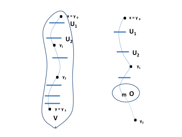
Figure 1.

For a system $(\underline{\gamma},V,\underline{U})$ with $V$ open neighborhood of $\underline{\gamma}$ in $M$ and $\underline{U}$ a transversal slice to $\underline{\gamma}\$ denote by $\mathcal{V}(\underline{\gamma},V,\underline{U})$ the collection of possibly broken instantons in $\hat{\mathcal{T}}(x,y)$ which lie inside $V$ and have $\underline{U}$ as a transversal slice.

For a system $(\tilde{\gamma},V,\underline{U},O)$ with $\tilde{\gamma}\in\hat{W}^{-}_{x},$ $V$ open neighborhood of $\tilde{\gamma}$ in $M$ $\underline{U}$ transversal slice for $(\gamma_{1},\cdots\gamma_{r},\gamma_{m})$ and $O$ an open neighborhood of $m,$ see FIGURE 1, denote by $\mathcal{V}(\tilde{\gamma},V,\underline{U},O)$ the collection of all elements in $\hat{W}^{-}_{x}$ which lie inside $V,$ have $\underline{U}$ as a transversal slice and have the end point in $O.$

A base of the transversal slice topology for $\hat{\mathcal{T}}(x,y)$ resp. for $\hat{W}^{-}_{x}$ is provided by the sets $\mathcal{V}(\underline{\gamma},V,\underline{U})$ for all systems $(\underline{\gamma},V,\underline{U})$ resp. the sets $\mathcal{V}(\tilde{\gamma},V,\underline{U},O)$ for all systems $(\tilde{\gamma},\ V,\underline{U},\ O).$

Theorem 1.3.

1. When equipped with the "transversal slice" topology the sets $\hat{W}^{\mp}_{x},\hat{\mathcal{T}}(x,y)$ and $\hat{\mathcal{M}}(x,z)$ are Haussdorf paracompact spaces and the maps $\hat{i}^{-}_{x}:\hat{W}^{-}_{x}\to M$ and $\hat{i}_{x,z}:\hat{\mathcal{M}}(x,z)\to M$ are continuous.

2. If $X$ admits Lyapunov function then $\hat{W}^{\mp}_{x},\hat{\mathcal{T}}(x,y)$ and $\hat{\mathcal{M}}(x,z)$ are compact.

Proof.

(sketch). Suppose first that $X$ admits a Lyapunov function $f:M\to\mathbb{R}.$

The case of $\hat{\mathcal{T}}(x,y)$: Suppose $f(x)=c_{1}$ and $f(y)=c_{2}$ and choose $\alpha_{0}<c_{1}<\alpha_{1}<\alpha_{2}<\cdots\alpha_{k-1}<c_{2}<\alpha_{k}$ with $\alpha_{i}$ regular values and with the intervals $(\alpha_{i},\alpha_{i+1})$ containing only one critical value $c_{i+1}.$ The map which assigns to a broken instanton $\underline{\gamma}$ its intersection with the levels $f^{-1}(\alpha_{i})^{\prime}s,$

$$i:\hat{\mathcal{T}}(x,y)\to\prod_{i=1,\cdots,(k-1)}f^{-1}(\alpha_{i}),$$

is a one to one map. It is not hard to see that the transversal slice topology is the same as the topology induced by this embedding. Indeed one can consider only transversals which lie in the levels $f^{-1}(\alpha_{i})$ and show they suffice to describe the transversal slice topology. Standard arguments cf. [3] show that the image of $i$ is closed hence compact. This proves the result for $\hat{\mathcal{T}}(x,y).$

The case of $\hat{W}^{-}_{x}:$ Write the critical values in decreasing order $\cdots>c_{i}>c_{i+1}>\cdots.$ Verify the first assertion in Theorem 1.3 for $(\hat{i}^{-}_{x})^{-1}(f^{-1}(a,b))$ instead of $\hat{W}^{-}_{x}$ when $a,b$ are regular values of $f$ with at most one critical value in the interval $(a,b).$ The set $(\hat{i}^{-}_{x})^{-1}(f^{-1}(a,b))$ can be embedded in a product of finitely many levels of $f$ and $M$ and one can check that the transversal slice topology and the topology induced by such embedding are the same. Since $\hat{i}^{-}_{x}$ is continuous w.r. to the transversal slice topology, hence $(\hat{i}^{-}_{x})^{-1}(f^{-1}(a,b))$ is open and $\hat{W}^{-}_{x}$ is covered by such sets, then the conclusion extends from $(\hat{i}^{-}_{x})^{-1}(f^{-1}(a,b))$ to $\hat{W}^{-}_{x}.$ The compacity assertion follows from the compacity of $(\hat{i}^{-}_{x})^{-1}(f^{-1}[\alpha,\beta]).$

To conclude the statement in general (when no Lyapunov function exists) one observes that any $\underline{\gamma}\in\hat{\mathcal{T}}(x,y),$ or $(\underline{\gamma},m)\in\hat{W}^{-}_{x}$ lies inside an open set $V$ of $M$ so that the vector field $X|_{V}$ admits Lyapunov function $f:V\to\mathbb{R}.$ This follows from the existence of Lyapunov functions in the neighborhood of each hyperbolic rest point a fact noticed above. More details will be contained in [5].

The main result of this paper states that the topological spaces $\hat{W}^{\pm}_{x},\ \hat{\mathcal{T}}(x,y)$ and $\hat{\mathcal{M}}(x,y)$ have structures of smooth manifold with corners. To explain this let us recall a few definitions.

The standard example and the local model of a smooth manifold with corners is

$$\mathbb{R}^{n}_{+}:=\{(x_{1},x_{2},\cdots x_{n})\in\mathbb{R}^{n}|x_{i}\geq 0\}.$$

The $k-$corner of $\mathbb{R}^{n}_{+}$ is

$${\partial_{k}\mathbb{R}^{n}_{+}:=\{x\in\mathbb{R}^{n}_{+}|\text{exactly}\ k\ \text{coordinates}\ x_{i}=0\}}.$$

Denote by $[[n]]$ the set $\{1,2,\cdots,n-1,n\}.$ If $I=\{{i_{1}},{i_{2}},\cdots{i_{k}}\}$ is a subset of $[[n]]$ denote by $\mathbb{R}^{I}$ the set of points in $\mathbb{R}^{n}_{+}$ whose coordinates $x_{i_{1}},x_{i_{2}},\cdots x_{i_{k}}$ are different from zero while all other coordinates vanish. Note that each $\mathbb{R}^{I}$ carries a canonical orientation defined by the order $i_{1}<i_{2},\cdots<i_{k}.$

A smooth manifold with corners is a Haussdorf paracompact space $P$ equipped with a differential structure locally isomorphic to $\mathbb{R}^{n}_{+}.$ A differential structure is given by an equivalence class of atlases. An atlas $\{\varphi_{\alpha}:U_{\alpha}\to V_{\alpha},\alpha\in\mathcal{A}\}$ consists of

an index set $\mathcal{A}$ ,

$U_{\alpha}\subseteq P$ open sets of $P,$

$V_{\alpha}\subseteq\mathbb{R}^{n}_{+}$ open sets of $\mathbb{R}^{n}_{+}$, and

$\varphi_{\alpha}$ homeomorphisms (charts)

so that $\cup_{\alpha}V_{\alpha}=P$ and $\varphi_{\beta}\cdot\varphi^{-1}_{\alpha}$ are smooth and of maximal rank where defined. Two atlases are equivalent if their data considered together remain an atlas.

The $k-$corner $\partial_{k}P$ is the set of points which in some chart (and then in any) correspond to $\partial_{k}\mathbb{R}^{n}_{+}.$

The manifold with corners is orientable if $\partial_{0}P$ is orientable. An orientation on such manifold is an orientation for its tangent bundle, equivalently an orientation of the open manifold $\partial_{0}P.$

A smooth manifold with corners $P$ is clean if the closure of each connected component of the corners is a smooth manifold with corners. The main result of this paper is the following:

Theorem 1.4.

Let $X$ be a smooth vector field satisfying $P_{1}$ and $P_{2}$ (defined before Theorem 1.2).

1. There exists a canonical structure of clean smooth manifold with corners on $\hat{W}^{\mp}_{x},\$ $\hat{\mathcal{T}}(x,y)$ and $\ \hat{\mathcal{M}}(x,y)$ with

$$\partial_{k}\hat{W}^{-}_{x}=W^{-}_{x}(k),\ \ \partial_{k}\hat{\mathcal{T}}(x,y)=\mathcal{T}(x,y)(k),\ \ \partial_{k}\hat{\mathcal{M}}(x,y)=\mathcal{M}(x,y)(k)$$

and $\ \hat{i}^{\mp}_{x}$ so that $\ \hat{i}_{x,y}$ are smooth maps.

2. If the rest points of $X$ are of Morse type there exists an additional structure of smooth manifold with corners (different but diffeomorphic to the structure stated in 1.) with the same corners and the identity map restricted to each $k-$corner a diffeomorphism.

3. Both $\hat{\mathcal{T}}$ and $\hat{\mathcal{M}}$ are equipped with (stable) framings. A collection of orientations $\{o_{x},x\in\mathcal{X}(X)\}$ on $W^{-}_{x}$ induces coherent orientations on $\hat{\mathcal{M}}(x,y)$ and $\hat{\mathcal{T}}(x,y)$ .

Theorem 1.4 is not new but in the generality formulated above inexistent in literature. In less generality it can be recovered from [6] and [1] for the gradient of a Morse function and from [2], [3], [4] or [6] for the gradient of a closed one form. The proof below is along the lines of [2] or [3]. In [5] the result will be proven for a more general class of vector fields, called HB (hyperbolic - Bott) vector fields. For these vector fields the set of rest points $\mathcal{X}(X)$ is a smooth submanifold with $D_{x}$ hyperbolic in normal directions of $\mathcal{X}(X).$

The smooth structure provided by Theorem 1.4 is not the only possible canonical smooth structure. In fact, in the case the rest points are of Morse type, Theorem 1.4 provides two such canonical structures never the same. However all smooth structures of manifold with corners on $\hat{W}^{\mp}_{x},\ \hat{\mathcal{M}}(x,y)$ or $\hat{\mathcal{T}}(x,y)$ which extend the smooth structure of $W^{\mp}_{x},\ {\mathcal{M}}(x,y)$ or ${\mathcal{T}}(x,y)$ are diffeomorphic. By elementary smoothing theory one can show that such diffeomorphisms can be chosen to be the identity on arbitrary closed subsets of the $\partial_{0}$ part.

Theorem 1.4 provides a source of new invariants which deserve attention and we plan to explore in future work. For example:

1. A Morse type complex can be assigned to a class of vector fields substantially larger than the gradient like vector fields. Its homology/cohomology referred to as the instanton homology (cohomology) might relate the topology of the manifold and the dynamics of $X$ in a more subtle way than in the case of gradient like vector fields. For example if $X$ is the gradient of a closed one form both the Novikov cohomology and the cohomology of $M$ twisted by a closed one form can be obtained as instanton homology/cohomology. More general vector fields lead to more subtle instanton homologies / cohomologies.

2. A chain/ cochain complex can be derived from the corners structure of the manifold with corners $\hat{\mathcal{T}}(x,y).$ The homology/cohomology of such a complex, referred to as the incidence cohomology seems natural to investigate. It carries significant dynamical information not obviously related to the topology of the manifold.

3. The stable framing of $\mathcal{T}(x,y)$ can be used to define elements in $\pi_{i}^{S}(\Omega M),$ the stable homotopy groups of the free loop space of $M.$ A parametrized version of such elements might provide a more analytic understanding of the relationship between the homotopy of the space of diffeomorphisms and the Waldhaussen K- theory of the underlying manifold.

Acknowledgement: I thank Stefan Haller for pointing out a number of errors and misprints in a previous version of this manuscript.

2. Some basic ODE

Recall that a linear transformation of $\mathbb{R}^{n}$ is hyperbolic if all its eigenvalues have non vanishing real part. The stable resp. unstable subspace, $\mathbb{R}^{+}\subseteq\mathbb{R}^{n}$ resp. $\mathbb{R}^{-}\subseteq\mathbb{R}^{n},$ are the sum of generalized eigenspaces corresponding to the eigenvalues with negative resp. positive real part.

Consider

1. $A\in M(n\times n;\mathbb{R})$ hyperbolic with stable space $\mathbb{R}^{+}=\mathbb{R}^{k}\times 0$ and unstable space $\mathbb{R}^{-}=0\times\mathbb{R}^{n-k},$

2. $g:\mathbb{R}^{n}\to\mathbb{R}^{n}=\mathbb{R}^{+}\times\mathbb{R}^{-}$ a smooth map with compact support with $g(0)=0$ and $D_{0}g=0.$ We write $g=(g^{+},g^{-}).$ We require in addition that $g^{+}(x^{+},0)=0,g^{-}(0,x^{-})=0.$

Let $X:\mathbb{R}^{n}\to\mathbb{R}^{n}$ be the smooth map defined by $X(x)=Ax+g(x).$ Regard $X$ as a smooth vector field on $\mathbb{R}^{n}.$ Clearly $0\in\mathbb{R}^{n}$ is a hyperbolic rest point and the only rest point in a small neighborhood of $0.$

Denote by

$$\gamma(t:p,q,T_{1},T_{2}):=(\gamma^{+}(t:p,q,T_{1},T_{2}),\gamma^{-}(t:p,q,T_{1},T_{2}))\in\mathbb{R}^{+}\times\mathbb{R}^{-}$$

$(p,q)\in\mathbb{R}^{+}\times\mathbb{R}^{-},$ $T_{1}<T_{2}$ a trajectory which satisfies

$$\gamma^{+}(T_{1}:p,q,T_{1},T_{2})=p,$$ (1)

$$\gamma^{-}(T_{2}:p,q,T_{1},T_{2})=q.$$

In general such trajectory might not exist and even if exists it might not be unique. However we have :

Theorem 2.1.

For any positive integer $N$ there exists $\epsilon,\rho,C>0$ so that : 1. For any $(p,q)\in D^{+}(\epsilon)\times D^{-}(\epsilon),$ the discs of radius $\epsilon$ in $\mathbb{R}^{+}\times R^{-},$ and any $T_{1}<T_{2}$ there exists a unique trajectory $\gamma(t:p,q,T_{1},T_{2}).$

2. Moreover the following estimates hold

$$||\mathbb{T}\gamma^{+}(t:p,q,T_{1},T_{2})||\leq\epsilon C^{-\rho(t-T_{1})}$$ (2)

$$||\mathbb{T}\gamma^{-}(t:p,q,T_{1},T_{2})||\leq\epsilon C^{\rho(t-T_{2})}$$

for $T_{1}<t<T_{2},$ where $\mathbb{T}=\frac{\partial^{k_{1}}}{\partial p^{k_{1}}}\frac{\partial^{k_{2}}}{\partial q^{k_{2}}}\frac{\partial^{k_{3}}}{\partial t^{k_{3}}}\frac{\partial^{k_{4}}}{\partial T_{1}^{k_{4}}}\frac{\partial^{k_{5}}}{\partial{T_{2}}^{k_{5}}}$ with $k_{1}+k_{2}+k_{3}+k_{4}+k_{5}\leq N$

The result is a straightforward application of contraction principle. A proof can be derived on the lines of the proof of Theorem A.2 and Lemma A.3 of Appendix of [1]. For the reader’s convenience we sketch the proof of (1.) and comment on the proof of (2.).

We continue to write $p$ and $g^{+}$ for $(p,0),$ and $(g^{+},0),$ and $q$ and $g^{-}$ for $(0,q)$ and $(0,g^{-}).$ We also write $\Psi(s,t)$ for $e^{(t-s)A}.$

Using the hyperbolic linear transformation $A$ one can produce the real numbers $\rho^{\prime}>0$ and $C>1$ so that

$$||\Psi(s,t)p|| \leq Ce^{-\rho^{\prime}(s-t)}||p||\ \text{for}\ s\geq t,$$ (3)

$$||\Psi(s,t)q|| \leq Ce^{\rho^{\prime}(s-t)}||q||\ \text{for}\ s\leq t.$$

Since the trajectory $\gamma(t):=\gamma(t,p,q,T_{1},T_{2})$ has to satisfy the equality

$$\gamma(t)=\Psi(t,T_{1})(p)+\Psi(t,T_{2})(q)+\int_{T_{1}}^{t}\Psi(s,t)g^{+}(\gamma(s))ds-\int_{t}^{T_{2}}\Psi(s,t)g^{-}(\gamma(s))ds$$ (4)

one concludes that $\gamma(t)$ is a fixed point of the map $F:C^{0}([T_{1},T_{2}],\mathbb{R}^{n})\to C^{0}([T_{1},T_{2}],\mathbb{R}^{n})$ defined by

$$F(x(t))=\Psi(t,T_{1})(p)+\Psi(t,T_{2})(q)+\int_{T_{1}}^{t}\Psi(s,t)g^{+}(x(s))ds-\int_{t}^{T_{2}}\Psi(s,t)(0,g^{-}(x(s))ds.$$ (5)

Choose $B>0$ so that

$$||Dg(x)||\leq B||x||.$$

Then if $||(p,q)||\leq\epsilon$ and $||x(t)||\leq\eta$ one has

$$||F(x(t)||\leq 2C\epsilon+\frac{2CB\eta^{2}}{\rho^{\prime}}.$$ (6)

One can find $\eta$ and $\epsilon^{\prime}$ small so that $F$ sends the disc of radius $\eta$ into itself provided $||(p,q)||\leq\epsilon^{\prime}$. Precisely one chooses $\eta$ to satisfy

$$\eta\leq\frac{\rho^{\prime}}{4BC},$$

and $\epsilon^{\prime}$ to satisfy

$$\epsilon^{\prime}<\frac{\eta}{4C}.$$

These choices make both terms of the right side of the above inequality (6) smaller than $\eta/2.$ Then $||x(t)||\leq\eta$ implies $||F(x(t))||\leq\eta.$

Note that the estimates remain true for any $\eta^{\prime}\leq\eta$ (when $\epsilon^{\prime}$ is appropriately chosen). Since we have

$$||\frac{\partial F}{\partial x}||\leq CB\eta/2\rho^{\prime}(1-e^{\rho^{\prime}(T_{1}-t)})+CB\eta/2\rho^{\prime}\leq CB\eta/\rho^{\prime}<1/4$$ (7)

by choosing $\eta<\rho^{\prime}/4CB$ and $\epsilon^{\prime}<\eta/4C$ one concludes that $F$ sends the disc $\mathbb{D}(\eta)$ of radius $\eta$ (in the complete metric space $C^{0}([T_{1},T_{2}],\mathbb{R}^{n})$) into itself and that $F:\mathbb{D}(\eta)\to\mathbb{D}(\eta)$ is a contraction.

To prove (2.) we first produce $\epsilon$, $\rho$ with $\epsilon<\epsilon^{\prime}$, $\rho<\rho^{\prime}$ so that (2) are satisfied for $N=0,$ then decrease $\epsilon$ and $\rho$ inductively with $N$ to satisfy (2.)

This is done by incorporating the estimates stated in (2.) in the definition of the metric space $C^{0}([T_{1},T_{2}],\mathbb{R}^{n}),$ and decrease $\epsilon,\rho$ to make sure that $F$ remains a contraction even in the presence of these estimates, hence the unique fixed point $\gamma$ satisfies the estimates.

3. Elementary differential topology of smooth manifolds with corners

If $P$ is a smooth manifold with corners then:

$\partial_{k}P$ is a a smooth $(n-k)-$manifold,

$\partial P:=\bigsqcup_{k\geq 1}\partial_{k}P$ is a topological $(n-1)-$manifold, and

$(P,\partial P)$ is a smoothable topological manifold with boundary.

If $P_{i},$ $i=1,2$ are two smooth manifolds with corners then the product $P_{1}\times P_{2}$ is a smooth manifold with corners with

$$\partial_{k}(P_{1}\times P_{2})=\bigsqcup_{r=k^{\prime}+k^{\prime\prime}}\partial_{k^{\prime}}P_{1}\times\partial_{k"}P_{2}.$$

If both $P_{1}$ and $P_{2}$ are clean then so is the product.

Let $P$ be a smooth manifold with corners, $M$ a smooth manifold, $S\subseteq M$ a smooth submanifold and $f:P\to M$ a smooth map.

Definition 3.1.

The map $f$ is transversal to $S$, written $f\pitchfork S$, if $f|_{\partial_{k}P}\pitchfork S$ for any $k=0,1,\cdots n.$

Let $P_{i},$ $i=1,2$ be two smooth manifolds with corners, $M$ a smooth manifold and $f_{i}:P_{i}\to M$ smooth maps.

Definition 3.2.

The maps $f_{i}:P_{i}\to M$ are transversal, written $f_{1}\pitchfork f_{2},$ if the product $f_{1}\times f_{2}:P_{1}\times P_{2}\to M\times M$ is transversal to the diagonal $\Delta_{M}:=\{(x,x)\in M\times M|x\in M\}$ $(f_{1}\times f_{2}\pitchfork\Delta_{M}).$

The above definition can be extended to a finite set of smooth maps $f_{i}:P_{i}\to M$ from manifolds with corners $P_{i}$ to a smooth manifold $M.$

Theorem 3.3.

1. If $f\pitchfork S$ then $f^{-1}(S)$ is a smooth manifold with corners (smooth submanifold of $P$) with $\partial_{k}f^{-1}(S)=(f|_{\partial_{k}P})^{-1}(S).$ Moreover if $P$ is clean then so is $f^{-1}(S).$

2. If $f_{1}\pitchfork f_{2}$ then

$$(f_{1}\times f_{2})^{-1}(\Delta_{M}):=\{(u,v)\in P_{1}\times P_{2}|f_{1}(u)=f_{2}(v)\}$$

is a smooth manifold with corners. Moreover if $P_{i}$ are clean so is $(f_{1}\times f_{2})^{-1}(\Delta_{M}).$

Suppose $P$ is an oriented clean smooth manifold with corners. An orientation of $P$ induces an orientation on $\partial_{1}P$ and therefore an orientation on each component of $\partial_{1}P.$ Let $\alpha_{1}$ and $\alpha_{2}$ be two components of $\partial_{1}P$ and $\beta$ a component of $\partial_{2}P$. Suppose that $\beta\subset\overline{\alpha}_{1}$ and $\beta\subset\overline{\alpha}_{2}.$ Clearly $\beta$ is a codimension one submanifold of the $\partial_{1}P.$ Then an orientation $o$ on $P$ induces an orientation $o_{\alpha_{1}}$ on $\alpha_{1}$ which in turn induces an orientation $o^{1}_{\beta}$ on $\beta.$ Similarly the orientation on $P$ induces an orientation $o_{\alpha_{2}}$ on $\alpha_{2}$ which in turn induces an orientation $o^{2}_{\beta}$ on $\beta.$ Observe that the orientations $o^{1}_{\beta}$ and $\o^{2}_{\beta}$ are opposite.

Suppose now that $P$ is a compact orientable clean smooth manifold with corners of dimension $n.$

Fix an orientation $o_{\alpha}$ on each component $\alpha$ of the corners. Each component $\alpha$ of $\partial_{k}P$ is a smooth manifold of dimension $n-k.$ Denote by $\mathcal{P}_{k}$ the set of components of dimension $k$ (the components of $\partial_{n-k}P$).

Let $I_{k}:\mathcal{P}_{k}\times\mathcal{P}_{k-1}\to\mathbb{Z}$ be the function defined by

$$I_{k}(\alpha,\beta)={\begin{cases}0\ if\beta\nsubseteq\overline{\alpha}&\\ +1\ if\beta\subset\overline{\alpha}&\text{ and}\ o_{\alpha}\ \text{ induces}\ o_{\beta}\\ -1\ if\beta\subset\overline{\alpha}&\text{ and}\ o_{\alpha}\ \text{ induces the oposite of }o_{\beta}\end{cases}}$$

$\alpha\in\mathcal{P}_{k},\beta\in\mathcal{P}_{k-1}.$

The above observation implies that

$$\sum_{\beta\in\mathcal{P}_{k}}I_{k+1}(\alpha^{\prime},\beta)\cdot I_{k}(\beta,\alpha^{\prime\prime})=0$$ (8)

for any $\alpha^{\prime}\in\mathcal{P}_{k+1},$ $\alpha^{\prime\prime}\in\mathcal{P}_{k-1}.$

If for a commutative ring $\kappa$ one considers the $\kappa-$module

$$C^{k}:=\text{Maps}(\mathcal{P}_{k},\kappa)$$

and the linear maps $d^{k}:C^{k}\to C^{k+1}$ defined by

$$d^{k}(f)(\alpha)=\sum_{\beta\in\mathcal{P}_{k}}I_{k+1}(\alpha,\beta)f(\beta)$$

$f\in C^{k},$ then the equality (8) implies that $(C^{k},d^{k})$ is a cochain complex.

The cohomology of this cochain complex is called the incidence cohomology of the manifold with corners $P.$ This cohomology is independent on the chosen orientations $o_{\alpha}^{\prime}$s.

4. Proof of the main theorem

We will prove Theorem 1.4 only for $\hat{W}^{-}_{x}$ and $\hat{\mathcal{T}}(x,y).$ The statements for $\hat{W}^{+}_{x}$ will follow by changing $X$ into $-X$ since the stable sets for $X$ are the unstable sets for $-X.$ The statements for $\hat{\mathcal{M}}(x,y)$ can be verified in essentially the same way as for $\hat{\mathcal{T}}(x,y).$ Alternatively they can be derived from the statements about $\hat{W}^{-}_{x}$ and $\hat{W}^{+}_{y}$ in view of the fact that $\hat{\mathcal{M}}(x,y)=(\hat{i}^{-}_{x}\times\hat{i}^{+}_{y})^{-1}(\Delta_{M})$ consists of the pairs of points in the product $\hat{W}^{-}_{x}\times\hat{W}^{+}_{y}$ equalized by $\hat{i}^{-}_{x}$ and $\hat{i}^{+}_{y}.$

We will focus the attention to the assertions (1.) and (2.). Part of the assertion (3.), the orientability and the existence of the stable framing follow from the simple observation that $\mathcal{T}(x,y)\times W^{-}_{y}$ is an open set of $\partial_{1}\hat{W}^{-}_{x}.$ The last part, the compatibility of the stable framings and of the orientability of $\mathcal{T}(x,y)$ for various $x,y$ is a tedious but conceptually straightforward verification. More details will be provided in the expanded version of this work, cf. [5], which treats the more general case of Bott - hyperbolic vector fields.

We first prove assertions (1.) and (2.) under the additional hypothesis H.

Hypothesis H: $X$ admits a proper Lyapunov function $f:M\to\mathbb{R}$ which in the neighborhood of rest points, in convenient coordinates $u_{1},\cdots,u_{k},v_{1},\cdots,v_{n-k}$, is given by the quadratic expression

$$f(x_{1},\cdots x_{n})=c-\sum_{i=1}^{k}u_{i}^{2}+\sum_{j=1}^{n-k}v_{j}^{2}.$$

We also suppose that with respect to these coordinates the unstable resp. the stable set of the rest points corresponds to $\mathbb{R}^{k}\times 0$ resp. $0\times\mathbb{R}^{n-k}.$

Let $\cdots c_{1}<c_{2}<\cdots c_{k}<c_{k+1}\cdots$ be the set of critical values. Choose $\epsilon_{i}$ such that    $c_{i+1}-\epsilon_{i+1}>c_{i}+\epsilon_{i}.$

Introduce

$$M_{i}=f^{-1}(c_{i}),\ \ M_{i}^{\pm}=f^{-1}(c_{i}\pm\epsilon_{i}),\ \ M(i)=f^{-1}(c_{i-1},c_{i+1})$$

and denote by $\mathcal{X}(i)$ the set of rest points which lie in $M_{i},$ $\mathcal{X}(i)=\mathcal{X}\cap M_{i}.$ Denote by

$$\varphi_{k}:M_{k}^{-}\to M^{+}_{k-1}$$

the map defined by the flow of $X.$ Precisely $\varphi_{k}(x)$ is the intersection of the trajectory $\gamma_{x},\ x\in M^{-}_{k}$ with $M^{+}_{k-1},$ see FIGURE 2. below.

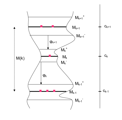
Figure 2.

For $x\in\mathcal{X}(i)$ denote by

$$S^{\pm}_{x}=M^{\pm}_{i}\cap W^{\pm}_{x},\ \ D^{\pm}_{x}=M(i)\cap W^{\pm}_{x},$$

see FIGURE 3. below,

$$\mathbb{S}^{\pm}_{i}:=\bigcup_{x\in\mathcal{X}(i)}S^{\pm}_{x},$$

$$\mathbb{D}^{\pm}_{i}:=\bigcup_{x\in\mathcal{X}(i)}D^{\pm}_{x},$$

$$(\mathbb{S}^{+}\rtimes\mathbb{S}^{-})_{i}:=\bigcup_{x\in\mathcal{X}(i)}S^{+}_{x}\times S^{-}_{x}.$$

$$(\mathbb{S}^{+}\rtimes\mathbb{D}^{-})_{i}:=\bigcup_{x\in\mathcal{X}(i)}S^{+}_{x}\times D^{-}_{x}.$$

Introduce the sets

$$P_{i}=\{(u,v)\in M^{+}_{i}\times M^{-}_{i}\mid u,v\ \text{lie on the same possibly broken trajectory}\},$$

$$Q_{i}=\{(u,v)\in M^{+}_{i}\times M(i)\mid u,v\ \text{ lie on the same possibly broken trajectory}\}.$$

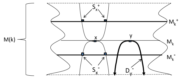
Figure 3.

Each set $P_{i}$ resp. $Q_{i}$ is a union of two disjoint subsets $\overset{\circ}{P_{i}}$ and $\partial P_{i}$ resp. $\overset{\circ}{Q_{i}}$ and $\partial Q_{i},$

$$\overset{\circ}{P}_{i}=\{(u,v)\in P_{i}\mid u,v\ \text{ lie on the same unbroken trajectory}\}$$

$$\partial P_{i}=\{(u,v)\in P_{i}\mid u,v\ \text{ lie on the same broken trajectory}\}$$

$$\overset{\circ}{Q}_{i}=\{(u,v)\in P_{i}\mid u,v\ \text{lie on the same unbroken trajectory}\}$$

$$\partial Q_{i}=\{(u,v)\in Q_{i}\mid u,v\ \text{ lie on the same broken trajectory}\}.$$

Equipped with the topology induced from the product $M^{+}_{i}\times M^{-}_{i}$ resp. $M^{+}_{i}\times M(i)$ $P_{i}$ resp. $Q_{i}$ is a topological manifold with boundary with $\overset{\circ}{P}_{i}\ \text{resp.}\ \overset{\circ}{Q}_{i}$ the interior and $\partial P_{i}\ \text{resp.}\ \partial Q_{i}$ the boundary. Actually both $\overset{\circ}{P}_{i}\ \text{and}\ \partial P_{i}$ resp.$\ \overset{\circ}{Q}_{i}\ \text{and}\ \partial Q_{i}$ are smooth submanifolds of $M^{+}_{i}\times M^{-}_{i}$ resp. $M^{+}_{i}\times M(i)$ but $P_{i}$ resp. $Q_{i}$ might not be in general.

For both $P_{i}$ and $Q_{i}$ denote by $p^{+}_{i}$ resp. $p^{-}_{i}$ the projection on the first resp. second component of $M^{+}_{i}\times M^{-}_{i}$ and $M^{+}_{i}\times M(i)$ and by $p_{i}=p^{+}_{i}\times p^{-}_{i}$ their product. The map $p_{i}$ is one to one and homeomorphism onto the image. In addition we have the following.

1. The map $p_{i}$ identifies $\partial P_{i}$ with $(\mathbb{S}^{+}\rtimes\mathbb{S}^{-})_{i},$ and $\partial Q_{i}$ with $(\mathbb{S}^{+}\rtimes\mathbb{D}^{-})_{i}.$

2. The restrictions of $p^{\pm}_{i}$ to $\overset{\circ}{P_{i}}$ are diffeomorphisms onto $M^{\pm}\setminus\mathbb{S}^{\pm}_{i}$ and the restrictions to $\partial P_{i},$ via the identification above, are the projections on $\mathbb{S}^{\pm}_{i}.$

3. The restriction of $p^{+}_{i}$ to $\overset{\circ}{Q_{i}}$ is a smooth bundle over $M^{+}_{i}\setminus\mathbb{S}^{+}_{i}$ with fiber an open interval and the restriction to $\partial Q_{i}$ is the projection on $\mathbb{S}^{+}_{i}.$

4. The restriction of $p^{-}_{i}$ to $\overset{\circ}{Q_{i}}$ is a diffeomorphism onto $M(i)\setminus\mathbb{D}^{-}_{i}$ and the restriction to $\partial Q_{i}$ is the projection on $\mathbb{D}^{-}_{i}.$

As pointed out above the subsets $p_{i}(P_{i})$ and $p_{i}(Q_{i})$ are not necessarily smooth submanifolds of $M^{+}_{i}\times M^{-}_{i}$ resp. $M^{+}_{i}\times M(i),$ however the following propositions will provide structures of smooth manifold with boundary on both $P_{i}$ and $Q_{i}$ which will make $p_{i}$ smooth maps.

Proposition 4.1.

The smooth map $p_{i}:\partial P_{i}\to M^{+}_{i}\times M^{-}_{i}$ admits smooth extensions $\tilde{p}_{i}:\partial P_{i}\times[0,\epsilon)\to M^{+}_{i}\times M^{-}_{i}$ so that:

1. the image is a neighborhood of $(\mathbb{S}^{+}\rtimes\mathbb{S}^{-})_{i}$ in $p_{i}(P_{i}),$

2. $\tilde{p}_{i}$ is injective,

3. $\tilde{p}_{i}$ restricted to $\partial P_{i}\times(0,\epsilon)$ is of maximal rank.

Proposition 4.2.

The smooth map $p_{i}:\partial Q_{i}\to M^{+}_{i}\times M(i)$ admits smooth extensions $\tilde{p}_{i}:\partial Q_{i}\times[0,\epsilon)\to M^{+}_{i}\times M(i)$ so that:

1. the image is a neighborhood of $(\mathbb{S}^{+}\rtimes\mathbb{D}^{-})_{i}$ in $p_{i}(Q_{i})$

2. $\tilde{p}_{i}$ is injective.

3. $\tilde{p}_{i}$ restricted to $\partial Q_{i}\times(0,\epsilon)$ is of maximal rank.

The proofs of these propositions will be given towards the end of the section.

Equip $P_{i}$ with the smooth structure defined by the atlas obtained from $\{\partial P_{i}\times[0,\epsilon),\tilde{p}_{i}\}$ and $\overset{\circ}{P_{i}}.$ Similarly equip $Q_{i}$ with the smooth structure defined by the atlas obtained from $\{\partial Q_{i}\times[0,\epsilon),\tilde{p}_{i}\}$ and $\overset{\circ}{Q_{i}}.$ Equivalently, regard $P_{i}$ resp. $Q_{i}$ obtained by glueing $\partial P_{i}\times[0,\epsilon)$ resp. $\partial Q_{i}\times[0,\epsilon)$ to $\overset{\circ}{P_{i}}$ resp. $\overset{\circ}{Q_{i}}$ via the diffeomorphisms provided by the restriction of $\tilde{p}_{i}$ to $\partial P_{i}\times(0,\epsilon)$ resp. to $\partial Q_{i}\times(0,\epsilon).$ These smooth structures will be denoted by $(P_{i})_{h}$ resp.$(Q_{i})_{h}.$

If the rest points of $X$ are of Morse type then we have the following.

Proposition 4.3.

If the rest points of $X$ are of Morse type then the image $p_{i}(P_{i})\subset M^{+}\times M^{-}_{i}$ resp. $p_{i}(Q_{i})\subset M^{+}\times M(i)$ are smooth submanifolds with boundaries.

The proof of this proposition will be given towards the end of the section.

This implies that $P_{i}$ resp. $Q_{i}$ have a smooth structure of manifold with boundary denoted by $(P_{i})_{m}$ resp. $(Q_{i})_{m}.$ The structures $(m)$ are $(h)$ are never the same but $id:(P_{i})_{h}\to(P_{i})_{m}$ and $id:(Q_{i})_{h}\to(Q_{i})_{m}$ are smooth homeomorphisms which restrict to diffeomorphisms on the interiors and on the boundaries.

Propositions 4.1, 4.2 and 4.3 imply that for any $(r,k)$ the product $\mathcal{P}:=A\times P_{r+k-1}\times P_{r+k-2}\cdots P_{k+1}\times B$ with $A$ a smooth manifold and $B$ a smooth manifold, possibly with boundary, is a smooth manifold with corners. The corner $\partial_{l}\mathcal{P}$ can be described as follows.

For any $i$ with $r+k-1\geq i\geq k+1$ denote by $R_{i}$ the subset of $P_{i}$ which is either the interior or the boundary of $P_{i}$ and by $R_{k}$ the subset of $B$ which is either the interior or the boundary of $B.$

Then the corner $\partial_{l}\mathcal{P}$ is the disjoint union of products $A\times R_{r+k-1}\times R_{r+k-2}\cdots R_{k+1}\times R_{k}$ with $l$ of the sets $R_{i}^{\prime}s$ being boundaries and the remaining $r-l$ being interiors. For example if $B$ is a smooth manifold with boundary and $l=1$

$$\partial_{1}\mathcal{P}= A\times\partial P_{r+k-1}\times\overset{\circ}{P}_{r+k-2}\times\cdots\overset{\circ}{P}_{k+1}\times\overset{\circ}{B}\sqcup$$

$$A\times\overset{\circ}{P}_{r+k-1}\times\partial P_{r+k-2}\times\cdots\overset{\circ}{P}_{k+1}\cdots\times\overset{\circ}{B}\sqcup\cdots$$

$$A\times\overset{\circ}{P}_{r+k-1}\times\overset{\circ}{P}_{r+k-2}\times\cdots\partial P_{k+1}\times\overset{\circ}{B}\sqcup$$

$$A\times\overset{\circ}{P}_{r+k-1}\times\overset{\circ}{P}_{r+k-2}\times\cdots\overset{\circ}{P}_{k+1}\times\partial B.$$

Suppose Propositions 4.1, 4.2, 4.3 were established. Here is the general scheme to verify (1.) and (2.) for $\hat{\mathcal{T}}(x,y)$ and $\hat{W}^{-}_{x}.$

For any $r,k\geq 0$ consider the diagram

FIGURE 4.

where $X^{\prime}s,Y^{\prime}s$ and $A$ are smooth manifolds, $Z^{\prime}s$ and $B$ smooth manifolds with boundary (possibly empty) and the arrows are smooth maps with $\varphi^{\prime}$s embeddings.

Denote by $\mathcal{S},\mathcal{O}$ and $\mathcal{P}$ the spaces defined by:

1. $\mathcal{S}=\mathcal{S}(r+k,k):=X_{r+k}\times X_{r+k-1}\times\cdots X_{k+1},$

2. $\mathcal{O}=\mathcal{O}(r+k,k):=X_{r+k}\times Y_{r+k-1}\times X_{r+k-1}\times\cdots X_{k+1}\times Y_{k},$

3. $\mathcal{P}=\mathcal{P}(r+k,k):=A\times Z_{r+k-1}\times Z_{r+k-2}\times\cdots Z_{k+1}\times B,$

Denote by $s$ and $t$ the maps defined by:

1. $s=s(r+k,k):\mathcal{S}\to\mathcal{O},$ the product of all maps from the top line to the middle line in the diagram above and

2. $t=t(r+k,k):\mathcal{P}\to\mathcal{O},$ the product of all maps from the bottom to the middle line in diagram above.

Since $id$ and $\varphi^{\prime}s$ are embeddings so is $s$ and $s(\mathcal{S})$ is a smooth submanifold of $\mathcal{O}.$ Note that $\mathcal{P}$ is a smooth manifold with corners, $\mathcal{O}$ and $\mathcal{S}$ are smooth manifolds, $t$ and $s$ are smooth maps.

We say that " the diagram FIGURE 4. is transversal" if $t\pitchfork s(\mathcal{S}).$ If so by Theorem 3.3, the subspace $t^{-1}(s(\mathcal{S}))$ receives a structure of smooth manifold with corners.

To accomplish the proof of (1.) and (2.) in Theorem 1.4 we choose the integers $r,k,$ the manifolds $X^{\prime}s,\cdots,B$ and the maps $\varphi_{i},p^{\pm}_{i},\alpha,\beta,$ appropriately in order to obtain $\hat{\mathcal{T}}(x,y)$ and $(\hat{i}_{x})^{-1}(f^{-1}(c_{r+k},c_{r})),$ as $t^{-1}(s(\mathcal{S})).$ Then we verify the transversality of the diagram FIGURE 4.

The case of $\hat{\mathcal{T}}(x,y).$ Choose $(r,k)$ so that $f(x)=c_{r+k}$ and $f(y)=c_{k}.$

Take $A=S^{-}_{x},$ $B=S^{+}_{y},$

$$(\varphi_{i+1}:X_{i+1}\to Y_{i})= (\varphi_{i+1}:M^{-}_{i+1}\to M^{+}_{i}),\ \ k\leq i\leq r+k-1,$$

$$(Z_{j},p^{+}_{j},p^{-}_{j})= (P_{j},p^{+}_{j},p^{-}_{j}),\ \ k+1\leq j\leq r+k-1.$$

Take $\alpha,\beta$ to be the obvious inclusions. With these choices $f^{-1}(s(\mathcal{S}))$ identifies with $\hat{\mathcal{T}}(x,y).$

Diagram FIGURE 4 becomes

FIGURE 5.

Then (1.) and (2.) follow from Proposition 4.4 below.

Proposition 4.4.

The diagram (FIGURE 5) is transversal.

Propositions 4.4 is a consequence of the transversality $i^{-}_{x}\pitchfork i^{+}_{y}$ for $x,y\in\mathcal{X}(X).$ For details the reader can consult [2] and [3].

The case of $\hat{W}^{-}_{x}:$ Let $f(x)=c_{m}$ and $k<m.$ This case is treated in two steps.

First we check that the open set $(\hat{i}_{x})^{-1}(M(k))$ has a structure of a smooth manifold with corners. For this purpose we use the same diagram (FIGURE 4) for $(r=m-k,k)$ $X,Y,Z,A,\alpha$ as in the case of $\hat{\mathcal{T}}(x,y),$ $B=Q_{k},$ $\beta=p^{+}_{k}:Q_{k}\to M^{+}_{k}$ and we replace Proposition 4.4 by Proposition 4.5 below. Diagram FIGURE 4 becomes

FIGURE 6.

Proposition 4.5.

The diagram (FIGURE 6) is transversal.

As with Proposition 4.4, Proposition 4.5 is a consequences of the transversality $i^{-}_{x}\pitchfork i^{+}_{y}$ for $x,y\in\mathcal{X}(X).$ For details the reader can consult [2] and [3].

Proposition 4.5 implies that $(\hat{i}_{x})^{-1}(M(k))$ has a structure of smooth manifold with corners.

Second, we verify that the smooth structures on $(\hat{i}_{x})^{-1}(M(k))$ and on $(\hat{i}_{x})^{-1}(M(k-1))$ agree. For this purpose we consider the map $h:=f\circ p^{-}_{i}:Q_{i}\to(c_{i+1},c_{i-1})$ and let $Q_{i}^{\prime}:=h^{-1}(c_{i+1},c_{i})$ and $Q_{i}^{\prime\prime}:=h^{-1}(c_{i},c_{i-1}).$ Both are open subsets of $Q_{i}$ and we have:

Observation 4.6.

There are canonical diffeomorphisms

$$\theta^{\prime}_{k}:Q_{k}^{\prime}\to M^{+}_{k}\times(c_{k+1},c_{k})$$

$$\theta^{\prime\prime}_{k}:Q_{k}^{\prime\prime}\to P_{k}\times_{M^{-}_{k}}(M^{-}_{k}\times(c_{k},c_{k-1}))$$

where the fiber product is taken with respect to $p^{-}_{k}:P_{k}\to M^{-}_{k}$ and the projection $M^{-}_{k}\times(c_{k},c_{k-1})\to M^{-}_{k}.$

Then the composition of :

1. $\theta_{k}^{\prime\prime}:Q_{k}^{\prime\prime}\to P_{k}\times_{M^{-}_{k}}(M^{-}_{k}\times(c_{k},c_{k-1})),$

2. the inclusion $P_{k}\times_{M^{-}_{k}}(M^{-}_{k}\times(c_{k},c_{k-1}))\subset P_{k}\times(M^{-}_{k}\times(c_{k},c_{k-1})),$

3. $id\times\varphi_{k-1}\times id:P_{k}\times M^{-}_{k}\times(c_{k},c_{k-1})\to P_{k}\times M^{+}_{k-1}\times(c_{k},c_{k-1})$ and

4. $id\times(\theta_{k-1}^{\prime})^{-1}:P_{k}\times M^{+}_{k-1}\times(c_{k},c_{k-1})\to P_{k}\times Q_{k-1}^{\prime}$

is a smooth embedding denoted by $\theta_{k}:Q_{k}^{\prime\prime}\to P_{k}\times Q_{k-1}^{\prime}.$

We write $t^{\prime}:\mathcal{P}^{\prime}\to\mathcal{O}$ resp. $t^{\prime\prime}:\mathcal{P}^{\prime\prime}\to\mathcal{O}$ instead of $t:\mathcal{P}\to\mathcal{O}$ and $Q^{\prime}$ resp. $Q^{\prime\prime}$ instead of $Q.$

In view of Observation 4.6 the map $\mathcal{P}^{\prime}(n,k)\to\mathcal{P}^{\prime\prime}(n,k-1),$ given by the product of $id^{\prime}s$ (on $S^{-}_{x},P_{n-1},\cdots P_{k-1}$) and of $\theta_{k}:Q_{k}^{\prime\prime}\to P_{k}\times Q_{k-1}^{\prime},$ is a smooth embedding which sends

$$(t^{\prime\prime}(n,k))^{-1}(s(n,k)(\mathcal{S}(n,k))$$

onto

$$(t^{\prime}(n,k-1))^{-1}(s(n,k-1)(\mathcal{S}(n,k-1)).$$

It identifies the structures of smooth manifolds with corners which were derived using $k$ and $k-1.$

Apparently the smooth structures defined so far depend on the Lyapunov function and the choices of $\epsilon_{i};$ this is not the case.

The independence of Lyapunov function: The arguments are the same for $\hat{\mathcal{T}}$ and $\hat{W}^{-}$ so we will treat only $\hat{\mathcal{T}}.$

If $f$ and $f^{\prime}$ are two Lyapunov functions and $\underline{\gamma}$ a possibly broken instanton we consider two transversals $\underline{V}=(V_{1},\cdots,V_{k})$ and $\underline{V}^{\prime}=(V^{\prime}_{1},\cdots V^{\prime}_{k})$ with the same mark points and $V_{i}$ contained in the levels of $f$ and $V^{\prime}_{i}$ contained in the levels of $f^{\prime}.$ We can find a diffeomorphism $\theta$ of a neighborhood $U$ of $\gamma$ onto a neighborhood $\theta(U)$ of $\gamma$ which restricts to the identity on $\gamma$ and sends $V_{i}$ into $V^{\prime}_{i}.$ This diffeomorphism provides an open embedding from the product of $V_{i}$ into the product of $V^{\prime}_{i}.$ It follows that $id:\hat{\mathcal{T}}\to\hat{\mathcal{T}}$ is smooth and of maximal rank in the neighborhood of $\underline{\gamma}$ with respect to either one of the smooth structure $(h)$ or $(m)$ defined using $f$ and $f^{\prime}.$ The removal of the additional hypothesis H: While global Lyapunov functions might not exist, for any broken instanton $\underline{\gamma}$ from the rest point $x$ to the rest point $y$ one can find an open neighborhood $U$ in $M$ so that a "convenient Lyapunov function" $f:U\to\mathbb{R}$ for $X|_{U}$ exists. Here "convenient Lyapunov function" means that the system $(X|_{U},f,U)$ is diffeomorphic to $(Y|_{V},g|_{V},V)$ where $Y$ is a smooth vector field satisfying $P_{1}$ and $P_{2}$ on a smooth manifold $N,$ $g:N\to\mathbb{R}$ a proper Lyapunov function for $Y$ and $V$ an open set in $N.$ As the space $\hat{\mathcal{T}}_{U}(x,y)$ consisting of broken instantons from $x$ to $y$ which lie in $U$ is an open set in $\hat{\mathcal{T}}(x,y)$ we define a smooth structure on $\hat{\mathcal{T}}_{U}(x,y)$ and note that for different such $U^{\prime}s$ these structures agree on intersections. The smooth structure on $\hat{\mathcal{T}}_{U}(x,y)$ is defined using the space of broken instantons of $Y$ on $N$ which lie in $V.$

Proof of Proposition 4.1, 4.2

First we introduce some notation. In the context of Theorem 2.1 in section 2 denote by $S^{\pm}$ and by $D^{\pm}$ the sphere and the disc of radius $\epsilon$ in $\mathbb{R}^{\pm}$ and when this notation is applied to coordinates about a rest point $x$ write $S^{\pm}_{x}$ and by $D^{\pm}_{x}$ instead.

Define the maps $\chi_{1}=(\chi^{+}_{1},\chi^{-}_{1}):S^{+}\times D^{-}\times[0,\infty)\to(\mathbb{R}^{+}\times\mathbb{R}^{-})$ and $\chi_{2}=(\chi^{+}_{2},\chi^{-}_{2}):S^{+}\times D^{-}\times[0,\infty)\to(\mathbb{R}^{+}\times\mathbb{R}^{-}),$ by the formulae:

$$\chi_{1}^{+}(p,q,s)= p$$ (9)

$$\chi_{1}^{-}(p,q,s)= \gamma^{-}(-1/s,p,q,-1/s,1/s)\text{\ }ifs\neq 0$$

$$\chi_{1}^{-}(p,q,0)= 0$$

$$\chi_{2}^{+}(p,q,s)= \gamma^{+}(1/s,p,q,-1/s,1/s)\text{\ }ifs\neq 0$$ (10)

$$\chi_{2}^{-}(p,q,0)= 0$$

$$\chi_{2}^{-}(p,q,s)= q.$$

Define $\chi:=(\chi_{1},\chi_{2}):S^{+}\times D^{-}\times[0,\infty)\to(\mathbb{R}^{+}\times\mathbb{R}^{-})\times(\mathbb{R}^{+}\times\mathbb{R}^{-}).$

Clearly $\chi(S^{+}\times S^{-}\times[0,\infty))\subset(S^{+}\times\mathbb{R}^{-})\times(\mathbb{R}^{+}\times\mathbb{S}^{-}).$

The estimates in Theorem 2.1 show that the map $\chi$ is smooth and for $\theta$ small the restriction of $\chi$ to $S^{+}\times S^{-}\times(0,\theta)$ and to $S^{+}\times S^{-}\times 0$ is of maximal rank but $\chi$ is not. It fails at the points of $S^{+}\times S^{-}\times 0.$ Example : If

$$X=-\operatorname{grad}f=- \sum_{i=1}^{k}x_{i}\partial/\partial x_{j}+\sum_{j=k+1}^{n}x_{j}\partial/\partial x_{j}.$$ (11)

$$p=(x_{1},\cdots x_{k}), \ q=(x_{k+1},\cdots,x_{n})$$

a simple calculation shows that:

$$\gamma^{+}(t;p,q,T_{1},T_{2})=e^{(T_{1}-t)}p,\ \ \gamma^{-}(t;p,q,0,T)=e^{-(T_{2}-t)}q.$$

The estimates in Theorem 2.1 are satisfied and $\chi$ is visibly not of maximal rank at the points of $S^{+}\times S^{-}\times 0.$

We proceed now with the proof of Propositions 4.1 and 4.2.

Observe that it suffices to check the statements in Propositions 4.1 and 4.2 for $\epsilon_{i}$ small enough and the statement in Proposition 4.2 for $M(i)$ replaced by the smaller open set $f^{-1}(c_{i}-\epsilon_{i},c_{i}+\epsilon_{i}).$

Choose for each rest point $x\in\mathcal{X}(i)$ a neighborhood and coordinates in the neighborhood so that the hypotheses of Theorem 2.1 are satisfied and $f=c_{i}-1/2|p|^{2}+1/2|q|^{2}.$ Here $|p|$ and $|q|$ denote the norm in the respective coordinates. Choose $\epsilon_{i}=\epsilon/2$ with $\epsilon$ small enough to have the conclusions of Theorem 2.1 satisfied for each rest point.

Since there is no risk of confusion from now on we drop the index $i$ from notation and write $M(\epsilon)$ instead of $f^{-1}(c_{i}-\epsilon,c_{i}+\epsilon).$

Define $u^{+}_{x}:S^{+}_{x}\times D^{-}_{x}\to M^{+},\text{resp}.\ u^{-}_{x}:D^{+}_{x}\times S^{-}_{x}\to M^{-}$ to be the map which assigns to $(p,q)$ the intersection of the trajectory through $(p,q)$ with $M^{+}$ resp. $M^{-}.$ The maps $u^{+}_{x}$ and $u^{-}_{x}$ are diffeomorphisms on their images and their restrictions to $S^{+}_{x}\times 0$ resp. to $0\times S^{-}_{x}$ are the identity maps.

For the rest point $x$ denote by $(\chi^{x}_{1},\chi^{x}_{2})$ the maps $(\chi_{1},\chi_{2})$ defined by the formulae (9) and (10).

For $P$ take $\tilde{p}_{x}:=(u^{+}_{x}\circ\chi^{x}_{1},u^{-}_{x}\circ\chi^{x}_{2}):S^{+}_{x}\times S^{-}_{x}\times[0,\epsilon^{\prime})\to M^{+}\times M^{-}$ and for $Q$ take $\tilde{p}_{x}:=(u^{+}_{x}\circ\chi^{x}_{1},\chi^{x}_{2}):S^{+}\times D^{-}_{x}\times[0,\theta)\to M^{+}\times M(\epsilon)$ with $\theta$ small enough to insure that the image of $S^{+}_{x}\times S^{-}_{x}\times[0,\theta)$ by $\chi^{x}_{2}$ lies in $M(\epsilon).$ Take $\tilde{p}=\sqcup_{x\in\mathcal{X}(i)}\tilde{p}_{x}.$ The maps $\tilde{p}$ satisfy the conclusions of Propositions 4.1 and 4.2.

Proof of Proposition 4.3: We use the same conventions and notations as in the previous proof.

The chosen neighborhoods and coordinates for the rest points are so made to have $X$ given by (11). Then, each trajectory of $X$ passing through $(p,q)\in\mathbb{R}^{n}\times\mathbb{R}^{n-k}$ ( $k=\operatorname{ind}x$) at $s=0$ is given by

$$\gamma(s)=(\gamma^{+}(s),\gamma^{-}(s)),\ \ \gamma^{+}(s)=e^{-s}p,\ \ \gamma^{-}(s)=e^{s}q.$$

To check that $P$ is a smooth submanifold with boundary it suffices to construct the smooth maps $\omega_{x}:S^{+}_{x}\times S^{-}_{x}\times[0,\epsilon)\to M^{+}\times M^{-}$ so that $\omega:(\mathbb{S}^{+}\rtimes\mathbb{S}^{-})\times[0,\epsilon)\to M^{+}\times M^{-}$ defined by $\omega=\sqcup_{x\in\mathcal{X}(i)}\omega_{x}$ satisfies:

1a. $\omega$ restricted to $\partial P=(\mathbb{S}^{+}\rtimes\mathbb{S}^{-})$ is the identity,

2a. the image of $\omega$ is an open neighborhood of $\partial P$ in $P.$

3a. $\omega$ is of maximal rank on $(\mathbb{S}^{+}\rtimes\mathbb{S}^{-})\times[0,\epsilon),$ (Note the distinction between item 3a. above and item 3. in Propositions 4.1 and 4.2.)

Define $u_{x}=(u^{+}_{x},u^{-}_{x})$ by assigning to $(p,q,t),$ $p\in S^{+}_{x},q\in S^{-}_{x}$ and $t\in[0,\epsilon)$ the pair of points provided by the intersection of the trajectory passing through $p+tq,$ with $M^{+}$ and $M^{-}.$ Define $\omega_{x}:=(u^{+}_{x}\circ\chi^{x}_{1},u^{-}_{x}\circ\chi^{x}_{2})$ where

$$\chi^{x}(p,q,t):=(\chi^{x}_{1}(p,q,t),\chi^{x}_{2}(p,q,t):=(p,tq,tp,q).$$

Items 1a., 2a, 3a. above are satisfied.

To check that $Q$ is a smooth submanifold with boundary it suffices to construct the smooth maps $\omega_{x}:S^{+}_{x}\times D^{-}_{x}\times[0,\epsilon)\to M^{+}\times M(\epsilon)$ so that $\omega=\sqcup_{x\in\mathcal{X}(i)}\omega_{x}$ satisfies:

1b. $\omega$ restricted to $\partial Q=(\mathbb{S}^{+}\rtimes\mathbb{D}^{-})$ is the identity,

2b. the image of $\omega$ is an open neighborhood of $\partial Q$ in $Q,$

3b. $\omega$ is of maximal rank on $(\mathbb{S}^{+}\rtimes\mathbb{D}^{-})\times[0,\epsilon).$

Define $u^{+}_{x}$ by assigning to $(p,q,t),$ $p\in S^{+}_{x},q\in D^{-}_{x}$ the intersection of the trajectory passing through $tp+q$ with $M^{+}.$ Define $\omega_{x}:=(u^{+}\circ\chi^{x}_{1},\chi^{x}_{2})$ where

$$\chi(u,v,t)=(\chi^{x}_{1}(p,q,t),\chi^{x}_{2}(p,q,t)):=((p,tq),(tp,q)).$$

Items 1b, 2b, 3b. above are satisfied.

q.e.d

Observation 4.7.

The reader can notice that the smooth structures (h) and (m) in the case of a vector field with the rest points of Morse type provided by Propositions 4.1, 4.2 and Proposition 4.3 respectively can not be the same.

References

[1]D.M. Austin and P.J. Braam,
Morse–Bott theory and equivariant cohomology.
The Floer memorial volume, 123–183.
Progr. Math. 133,
Birkhäuser, Basel, 1995.
[2] D.Burghelea. L. Friedlander, T. Kapeller
On the space of trajectories of a generic gradient like vector field
Analele Universitatii de Vest, Timisoara Seria Matematica – Informatica,
81 pages (to appear) (2010). This is a part of a book in preparation on Witten Deformation of the deRham complex.
[3]D. Burghelea S. Haller,
On the topology and analysis of closed one form. I (Novikov theory revisited),
Monogr. Enseign. Math. 38 (2001) 133–175.
[4]D. Burghelea S. Haller,
Dynamics Laplace transform and spectral geometry
Journal of Topology 1 (2008) 115-151.
[5]D. Burghelea S. Haller,
Bott hyperbolic vector fields
in preparation
[6] F. Latour
Existence de one-formes fermees non singulieres dans une classe de cohomologie de Rham
I.H.E.S. Publ. Math. 80. (1995) p 135-194.
[7]M.C. Irwin
Smooth Dynamical Systems
Academic Press 1980
[8]I. Kupka,
Contribution à la théorie des champs génériques,
Contributions to Differential Equations 2 (1963) 457–484.
[9]M.M. Peixoto,
On an Approximation Theorem of Kupka and Smale,
J. Differential Equations 3 (1967) 214–227.
[10]S. Smale,
Stable manifolds for differential equations and diffeomorphisms,
Ann. Scuola Norm. Sup. Pisa 17 (1963) 97–116.
[11]A. Katok B. Hasselblatt,
Introduction to the modern theory of Dynamical systems.
Cambridge University press, 1995.
[12]
M. Schwarz,
Morse homology.
Progress in Mathematics 111,
Birkhäuser Verlag, Basel, 1993.