Splitting of separatrices for the Hamiltonian-Hopf bifurcation with the Swift-Hohenberg equation as an example

Abstract

We study homoclinic orbits of the Swift-Hohenberg equation near a Hamiltonian-Hopf bifurcation. It is well known that in this case the normal form of the equation is integrable at all orders. Therefore the difference between the stable and unstable manifolds is exponentially small and the study requires a method capable to detect phenomena beyond all algebraic orders provided by the normal form theory. We propose an asymptotic expansion for an homoclinic invariant which quantitatively describes the transversality of the invariant manifolds. We perform high-precision numerical experiments to support validity of the asymptotic expansion and evaluate a Stokes constant numerically using two independent methods.

1 The generalized Swift-Hohenberg equation

The generalized Swift-Hohenberg equation (GSHE),

$$u_{t}=\epsilon u+\kappa u^{2}-u^{3}-(1+\Delta)^{2}u$$ (1)

is widely used to model nonlinear phenomena in various areas of modern Physics including hydrodynamics, pattern formation and nonlinear optics (e.g. [5, 14]). This equation (with $\kappa=0$) was originally introduced by Swift and Hohenberg [24] in a study of thermal fluctuations in a convective instability.

In the following we consider $u$ to be one dimensional and study stationary solutions of (1) which satisfy the ordinary differential equation

$$\epsilon u+\kappa u^{2}-u^{3}-(1+\partial^{2}_{x})^{2}u=0\,.$$ (2)

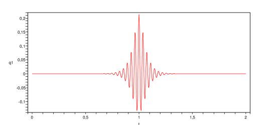
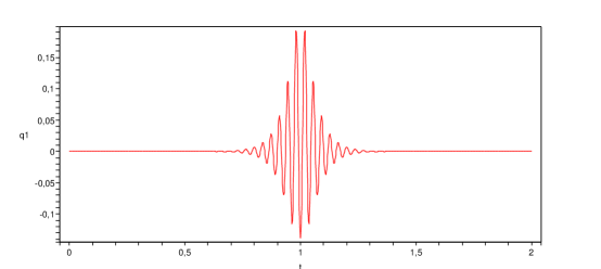
Obviously this equation has a reversible symmetry (if $u(x)$ satisfy the equation then $u(-x)$ also does). It is well known that for small negative $\epsilon$ this equation has two symmetric homoclinic solutions [13] similar to the ones shown on Figure 1. In this paper we study transversality of the homoclinic solutions, which implies existence of multi-pulse homoclinic solutions and a small scale chaos.

Figure 1: Two primary symmetric homoclinic solutions of the scalar stationary GSHE ($\epsilon=-0.05$ and $\kappa=2$).

In order to describe the homoclinic phenomena it is convenient to rewrite the equation (2) in the form of an equivalent Hamiltonian system [2, 19]:

$$\dot{q_{1}} =q_{2} \dot{p_{1}} =p_{2}-\epsilon q_{1}-\kappa q_{1}^{2}+q_{1}^{3}$$ (3)

$$\dot{q_{2}} =p_{2}-q_{1} \dot{p_{2}} =-p_{1}\,,$$

where the variables are defined by the following equalities

$$u=q_{1},\quad u^{\prime}=q_{2},\quad-(u^{\prime}+u^{\prime\prime\prime})=p_{1}\quad\mathrm{and}\quad u+u^{\prime\prime}=p_{2}$$ (4)

and the Hamiltonian function has the form

$$H_{\epsilon}=p_{1}q_{2}-p_{2}q_{1}+\frac{p_{2}^{2}}{2}+\epsilon\frac{q_{1}^{2}}{2}+\kappa\frac{q_{1}^{3}}{3}-\frac{q_{1}^{4}}{4}.$$ (5)

The system (3) is reversible with respect to the involution,

$$S:(q_{1},q_{2},p_{1},p_{2})\rightarrow(q_{1},-q_{2},-p_{1},p_{2}).$$

The origin is an equiblibrium of the system and the eigenvalues of the linearized vector field are

$$\left\{\pm\sqrt{-1+\sqrt{\epsilon}},\,\pm\sqrt{-1-\sqrt{\epsilon}}\right\}\,.$$

If $\epsilon<0$, the eigenvalues form a quadruple $\pm\beta_{\epsilon}\pm i\alpha_{\epsilon}$ where

$$\beta_{\epsilon} = \frac{\sqrt{2\sqrt{1-{\it\epsilon}}-2}}{2}=\sqrt{-\frac{\epsilon}{4}}\,(1+O(\epsilon))\,,$$

$$\alpha_{\epsilon} = \frac{\sqrt{2\sqrt{1-{\it\epsilon}}+2}}{2}=1+O(\epsilon)\,.$$

At $\epsilon=0$ the eigenvalues collide forming two purely imaginary eigenvalues $\pm i$ of multiplicity two. Moreover, the corresponding linearization of the vector field is not semisimple. Thus, the equilibrium point of system (3) undergoes a Hamiltonian-Hopf bifurcation described in the book [21] (see also [23]). In general position there are two possible scenarios of the bifurcation depending on the sign of a certain coefficient of a normal form. In the Swift-Hohenberg equation both scenarios are possible and depend on the value of the parameter $\kappa$. In this paper we will consider the case when the equilibrium is stable at the moment of the bifurcation (see [25, 20] for more details) which corresponds to $|\kappa|>\sqrt{\frac{27}{38}}$ as shown in [2]. Also note that the degenerate case $|\kappa|=\sqrt{\frac{27}{38}}$ leads to some interesting phenomena including “homoclinic snaking” [26, 18, 8].

When $\epsilon<0$ is small, the equilibrium is a saddle-focus and the Stable Manifold Theorem implies the existence of two-dimensional stable $\mathbf{W}_{\epsilon}^{s}$ and unstable $\mathbf{W}_{\epsilon}^{u}$ manifolds for the equilibrium point. These manifolds are contained inside the zero energy level of the Hamiltonian $H_{\epsilon}$.

The original Hamiltonian (5) can be seen as a perturbation of an integrable Hamiltonian which can be derived from the normal form theory (see section 1.2 for details). Since the normal form is integrable, its stable and unstable manifolds coincide (see also discussion in [17] for the reversible set up). In [13], Glebsky and Lerman used the implicit function theorem to prove the existence of two reversible (symmetric) homoclinic orbits for the original system (3) when $\epsilon<0$ is small. As a matter of fact, this result follows from a more general study concerning a 1:1 resonance in four dimensional reversible vector fields (see [17]). Also the paper [13] conjectures that the stable and unstable manifolds should intersect transversely yielding, in particular, the existence of countably many reversible homoclinic orbits. These orbits are known as multisolitons for the Swift-Hohenberg equation and they have been the subject of study in several works (see [6] and the references therein).

Note that no conclusion about the transversality of stable and unstable manifolds can be made using only the normal form theory. In this paper we study the splitting of the stable and unstable manifolds which happens beyond all orders of the normal form theory. Let $\mathbf{p}_{\epsilon}$ be a symmetric homoclinic point belonging to one of the two primary symmetric homoclinic orbits. In section 1.1 we propose a natural way to select vectors $v^{u,s}_{\epsilon}$ tangent to $\mathbf{W}_{\epsilon}^{s}$ and $\mathbf{W}_{\epsilon}^{u}$ at $\mathbf{p}_{\epsilon}$ (see equation (11)). The main goal of this paper is to establish the following asymptotic formula for the value of the standard symplectic form on this pair of vectors:

$$\Omega(v^{u}_{\epsilon},v^{s}_{\epsilon})=e^{-\frac{\pi\alpha_{\epsilon}}{2\beta_{\epsilon}}}\left(\omega_{0}(\kappa)+O(\epsilon)\right)\,.$$ (6)

Note that $\mathbf{W}_{\epsilon}^{s}$ and $\mathbf{W}_{\epsilon}^{u}$ are two dimensional Lagrangian manifolds confined inside the three dimensional energy level $\{H_{\epsilon}=0\}$. These manifolds intersect along homoclinic orbits. Their intersection along the orbit of $\mathbf{p}_{\epsilon}$ is transverse (inside the energy level) provided $\Omega(v^{u}_{\epsilon},v^{s}_{\epsilon})\neq 0$. If $\omega_{0}(\kappa)\neq 0$, the asymptotic formula (6) implies the transversality of the homoclinic orbit for small negative $\epsilon$, and therefore $\omega_{0}(\kappa)$ is known as the splitting coefficient.

We stress that the derivation of formula (6) does not rely substantially on the specific form of the Swift-Hohenberg equation and exactly the same asymptotic expression (only the splitting coefficient may take different values) can be deduced for a generic analytic family of reversible Hamiltonian systems undergoing a subcritical Hamiltonian-Hopf bifurcation. The details can be found in [9], where a majority of the arguments presented in this paper have been transformed into rigorous mathematical proofs.

In this paper, the derivation of formula (6) is not rigorous, as it is based on numerous estimates and assumptions which are not proved here. Nevertheless similar statements were proved in a similar context for other problems [10, 11].

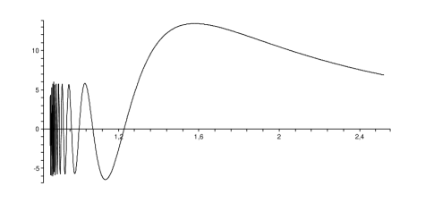
Supporting the validity of formula (6) we perform a set of numerical experiments and compute the splitting coefficient using two distinct methods. This constant is related to a purely imaginary Stokes constant, and Figure 2 gives an idea about its behaviour as a function of the parameter $\kappa$. The value of the Stokes constant comes from the study of the Hamiltonian (5) at the exact moment of the bifurcation (i.e. at $\epsilon=0$). We will discuss the relevant definitions in section 1.3 and some methods for its numerical evaluation in section 2.

Figure 2: Graph of the function $\mathrm{Im}(\Theta_{0}(\kappa))$ for $\kappa>\sqrt{\frac{27}{38}}$, $\omega_{0}(\kappa)=2\mathrm{Im}(\Theta_{0}(\kappa))$.

Recently, S. J. Chapman and G. Kozyreff [8] used the multiple-scales analysis beyond all orders to study localised patterns which emerge from a subcritical modulation instability in the Swift-Hohenberg equation. Their analysis captured exponentially small phenomena by means of optimal truncation of certain formal expansions combined with a study of their analytical continuation in a vicinity of the Sokes lines. Technically our approach is different and we do not require higher order terms, additionally our approach has the advantage of being directly applicable to study the exponentially small splitting of invariant manifolds near generic Hamiltonian-Hopf bifurcations, for which the Swift-Hohenberg is a particular example.

The rest of the paper is organised in the following way. In Section 1.1 we discuss the definition of an homoclinic invariant which provides a very convenient tool for measuring the splitting of invariant manifolds. In Section 1.2 we review some facts from the normal form theory which will be necessary for the exposition of our results. Section 1.3 contains the definition of the Stokes constant. An informal derivation of the asymptotic formula (6) which describes the splitting of invariant manifolds of the stationary Swift-Hohenberg equation near the Hamiltonian-Hopf bifurcation is placed in Section 1.4. As the derivation of the asymptotic formula is not rigorous we perform a set of high-precision numerical experiments in order to confirm its validity. Moreover, similar to many other problems which involve exponentially small splitting of invariant manifolds [11], the asymptotic formula contains a splitting coefficient which comes from an auxiliary problem and requires numerical evaluation. The results of our numerical experiments are reported in Sections 2 and 3.

1.1 Homoclinic invariant

In a study of homoclinic trajectories, both numerical and analytical, it is usually important to have a convenient basis in the tangent space to the stable and unstable manifolds. Below we provide a definition adapted to our problem. This definition can be of independent interest as it can be easily extended onto hyperbolic equilibria of higher dimensional systems (not necessarily Hamiltonian).

Suppose that the origin is an equilibrium of a Hamiltonian vector field $X_{H}$ and that $\pm\beta\pm i\alpha$ are the eigenvalues of $DX_{H}(0)$. Then the origin has a two dimensional stable manifold. According to Hartman [15] the restriction of the vector field on $W^{s}_{loc}$ can be linearised by a $C^{1}$ change of variables. In the polar coordinates the linearised dynamics on $W^{s}_{loc}$ takes the form:

$$\dot{r}=-\beta r\,\qquad\dot{\varphi}=\alpha\,.$$

It is convenient to introduce $z=-\ln r$ so that

$$\dot{z}=\beta\,.$$

Then the local stable manifold is the image of a function

$$\Gamma^{s}:\{(\varphi,z):\varphi\in S^{1},z>-\log r_{0}\}\to\mathbb{R}^{4}$$

where $r_{0}$ is the radius of the linearisation domain and $S^{1}$ is the unit circle. Since $\Gamma^{s}$ maps trajectories into trajectories we can propagate it uniquely along the trajectories of the Hamiltonian system using the property

$$\Gamma^{s}(\varphi+\alpha t,z+\beta t)=\Phi^{t}_{H}\circ\Gamma^{s}(\varphi,z)$$ (7)

where $\Phi^{t}_{H}$ is the flow defined by the Hamiltonian equation. Note that

$$\Gamma^{s}(\varphi+2\pi,z)=\Gamma^{s}(\varphi,z)$$

since $\varphi$ is the angle component of the polar coordinates. Moreover,

$$\lim_{z\to+\infty}\Gamma^{s}(\varphi,z)=0\,.$$

Differentiating $\Gamma^{s}$ along a trajectory we see that it satisfies the non-linear PDE:

$$\alpha\partial_{\varphi}\Gamma+\beta\partial_{z}\Gamma=X_{H}(\Gamma)\,.$$ (8)

Each of the derivatives $\partial_{z}\Gamma^{s}$ and $\partial_{\varphi}\Gamma^{s}$ defines a vector field on $W^{s}$. The equation (7) implies that $\partial_{z}\Gamma^{s}$ and $\partial_{\varphi}\Gamma^{s}$ are invariant under the restriction of the flow $\Phi^{t}_{H}\Bigr{|}_{W^{s}}$.

We can define $\Gamma^{u}$ applying the same arguments to the Hamiltonian $-H$. In this case it is convenient to set $z=\ln r$ to ensure that $\Gamma^{u}$ satisfies the same PDE as $\Gamma^{s}$. In a reversible system with a reversing involution $S$, it is convenient to set

$$\Gamma^{u}(\varphi,z)=S\circ\Gamma^{s}(-\varphi,-z).$$ (9)

Now suppose that the system has a homoclinic trajectory $\gamma_{h}$. Let us choose a point $\mathbf{p}_{h}\in\gamma_{h}$. The freedom in the definition allows us to assume that $\mathbf{p}_{h}=\Gamma^{s}(0,0)=\Gamma^{u}(0,0)$ without loosing in generality. This condition completely eliminates the freedom from the definition of $\Gamma^{u}$ and $\Gamma^{s}$.

In a Hamiltonian system the symplectic form provides a natural tool for studying transversality of invariant manifolds. Thus we arrive at the following,

Definition (Homoclinic Invariant).

The homoclinic invariant $\omega$ is defined by the formula,

$$\omega=\Omega(\partial_{\varphi}\Gamma^{u}(0,0),\partial_{\varphi}\Gamma^{s}(0,0))\,.$$ (10)

This definition is a natural extension of the homoclinic invariant defined for homoclinic orbits of area-preserving maps [11].

In the left hand side of the asymptotic formula (6) we use the notation

$$v_{\epsilon}^{u,s}=\partial_{\varphi}\Gamma^{u,s}(0,0).$$ (11)

It is easy to see that $\omega$ takes the same value for all points of the homoclinic trajectory $\gamma_{h}=\{\Phi^{t}_{H}(\mathbf{p}_{h}):t\in\mathbb{R}\}$. Indeed it follows from (7) that

$$\partial_{\varphi}\Gamma^{s}(\alpha t,\beta t)=D\Phi^{t}_{H}(\mathbf{p}_{\epsilon})\partial_{\varphi}\Gamma^{s}(0,0),$$

and a similar identity is valid for the unstable manifold. Since the Hamiltonian flow $\Phi^{t}_{H}$ is symplectic, we conclude that $\Omega(\partial_{\varphi}\Gamma^{u}(\alpha t,\beta t),\partial_{\varphi}\Gamma^{s}(\alpha t,\beta t))=\Omega(\partial_{\varphi}\Gamma^{u}(0,0),\partial_{\varphi}\Gamma^{s}(0,0))=\omega$.

Since $\Gamma^{s}$ and $\Gamma^{u}$ are Lagrangian and belong to the energy level $H=H(0)$, which is three-dimensional, the inequality $\omega\neq 0$ implies the transversality of the homoclinic trajectory. Indeed, if $\omega\neq 0$, the vectors $\partial_{\varphi}\Gamma^{u}(0,0)$, $\partial_{\varphi}\Gamma^{s}(0,0)$ and $X_{H}(\mathbf{p}_{h})$ are linearly independent and therefore span the tangent space to the energy level at $\mathbf{p}_{h}$.

We note that we can define two vectors tangent to $W^{s}$ and another two vectors tangent to $W^{u}$ at $\mathbf{p}_{h}\in W^{s}\cap W^{u}$. So we could use

$$\omega_{x,y}:=\Omega(\partial_{x}\Gamma^{u}(0,0),\partial_{y}\Gamma^{s}(0,0)),\quad x,y\in\left\{\varphi,z\right\}$$ (12)

instead of $\omega$. But these invariants are not independent. Indeed,

$$\alpha\partial_{\varphi}\Gamma^{u}(0,0)+\beta\partial_{z}\Gamma^{u}(0,0)=\alpha\partial_{\varphi}\Gamma^{s}(0,0)+\beta\partial_{z}\Gamma^{s}(0,0)$$

as both expressions are equal to $X_{H}(\mathbf{p}_{h})$. Then equation (12) implies

$$\alpha^{2}\omega-\beta^{2}\omega_{z,z}=0,\quad\alpha\omega+\beta\omega_{\varphi,z}=0,\quad\alpha\omega+\beta\omega_{z,\varphi}=0.$$

In the derivation of these identities it is also necessary to take into account that $W^{u,s}$ are Lagrangian (i.e., the symplectic form $\Omega$ vanishes on their tangent spaces).

In the case of the Swift-Hohenberg equation the system of PDE (8) can be conveniently replaced by a single scalar PDE of higher order obtained from (2) by replacing $\partial_{x}$ with the differential operator

$$\partial=\alpha_{\epsilon}\partial_{\varphi}+\beta_{\epsilon}\partial_{z}.$$

Let us use $u^{\pm}_{\epsilon}$ to denote the first component of $\mathbf{\Gamma}^{u}_{\epsilon}$ and $\mathbf{\Gamma}^{s}_{\epsilon}$ respectively, then $u^{\pm}_{\epsilon}$ satisfies the equation

$$(1+\partial^{2})^{2}u=\epsilon u+\kappa u^{2}-u^{3}\,.$$ (13)

Its other components can be restored using (4). The Swift-Hohenberg equation is reversible and following (9) we define

$$u^{+}_{\epsilon}(\varphi,z)=u^{-}_{\epsilon}(-\varphi,-z)\,.$$

We also assume that $\mathbf{\Gamma}^{s}_{\epsilon}(0,0)=\mathbf{\Gamma}^{u}_{\epsilon}(0,0)$ is the primary symmetric homoclinic point. Then the formula for the homoclinic invariant can be rewritten in terms of $u^{-}$:

$$\omega=2\partial_{\varphi}\left((u^{-})^{2}+u^{-}\partial^{2}u^{-})\right)$$ (14)

where the derivatives are evaluated at $(\varphi,z)=(0,0)$.

1.2 Normal form of the Swift-Hohenberg equation

The most convenient description of the bifurcation is obtained with the help of the normal form. As a first step the quadratic part of the Hamiltonian (5) is normalised with the help of a linear symplectic transformation (similar to [4]):

$$T=\left(\begin{array}[]{cccc}0&-1/4\,\sqrt{2}&-1/2\,\sqrt{2}&0\\ \vskip 6.0pt plus 2.0pt minus 2.0pt\cr 1/4\,\sqrt{2}&0&0&1/2\,\sqrt{2}\\ \vskip 6.0pt plus 2.0pt minus 2.0pt\cr\sqrt{2}&0&0&0\\ \vskip 6.0pt plus 2.0pt minus 2.0pt\cr 0&-\sqrt{2}&0&0\end{array}\right)$$

which transforms (5) into

$$\begin{split}H_{\epsilon}=&-(q_{2}p_{1}-q_{1}p_{2})+\frac{1}{2}(q_{1}^{2}+q_{2}^{2})+\frac{1}{4}p_{1}^{2}\epsilon-\frac{\sqrt{2}}{12}\kappa p_{1}^{3}+\frac{1}{4}q_{2}p_{1}\epsilon-\frac{\sqrt{2}}{8}\kappa q_{2}p_{1}^{2}+\\ &\frac{1}{16}q_{2}^{2}\epsilon-\frac{\sqrt{2}}{16}\kappa q_{2}^{2}p_{1}-\frac{\sqrt{2}}{96}\kappa q_{2}^{3}-\frac{1}{16}p_{1}^{4}-\frac{1}{8}q_{2}p_{1}^{3}-\frac{3}{32}q_{2}^{2}p_{1}^{2}-\frac{1}{32}q_{2}^{3}p_{1}-\frac{1}{256}q_{2}^{4}\end{split}$$ (15)

where we keep the same notation for the variables. Note that the involution $S$ in the new coordinates takes the form

$$\tilde{S}:(q_{1},q_{2},p_{1},p_{2})\rightarrow(-q_{1},q_{2},p_{1},-p_{2}).$$ (16)

Now, with the quadratic part in normal form, we can apply the standard normal form procedure to normalize the Hamiltonian (15) up to any order: There is a near identity canonical change of variables $\Psi_{n}$ which normalizes all terms of order less than equal to $n$ and transforms the Hamiltonian to the following form:

$$H_{\epsilon}=H_{\epsilon}^{n}+\mathrm{higher}\ \mathrm{order}\ \mathrm{terms}$$ (17)

where

$$H_{\epsilon}^{n}=-I_{1}+I_{2}+\sum_{\begin{subarray}{c}3i+2j+2l\geq 4\\ i+j\geq 1\end{subarray}}^{n}a_{i,j,l}I_{1}^{i}I_{3}^{j}\epsilon^{l}$$

with

$$I_{1}=q_{2}p_{1}-q_{1}p_{2},\qquad I_{2}=\frac{q_{1}^{2}+q_{2}^{2}}{2},\qquad I_{3}=\frac{p_{1}^{2}+p_{2}^{2}}{2}.$$

This normalization preserves the reversibility with respect to the involution (16). In the case of the GSHE the normal form up to the order five has the form (see Appendix A for more details about the change of variables)

$$H_{\epsilon}^{5}=-I_{1}+\left(I_{2}+\frac{1}{4}\epsilon I_{3}+\eta I_{3}^{2}\right)+\left(\frac{1}{8}\epsilon I_{1}+\mu\,I_{1}{I_{3}}\right)\,.$$

The leading part of the normal form includes two parameters which can be explicitly expressed in terms of the original parameter $\kappa$:

$$\eta=4\left({\frac{19}{576}}{\kappa}^{2}-{\frac{3}{128}}\right)\quad\mathrm{and}\quad\mu=2\left({\frac{65}{864}}\,{\kappa}^{2}-{\frac{3}{64}}\right)\,.$$

The geometry of the invariant manifolds depends on the sign of $\eta$ [21]. In the case of GSHE, if

$$\left|\kappa\right|>\sqrt{\frac{27}{38}},$$

then $\eta>0$ [13], and the truncated normal form has a continuum of homoclinic orbits among which exactly two are reversible, i.e., symmetric with respect to the involution (16).

In order to describe the geometry of the invariant manifolds near the bifurcation it is convenient to introduce the new parameter $\epsilon=-4\delta^{2}$ and perform the standard scaling:

$$q_{1}=\delta^{2}Q_{1},\quad q_{2}=\delta^{2}Q_{2},\quad p_{1}=\delta P_{1},\quad p_{2}=\delta P_{2}\,.$$

This change of variables is not symplectic, nevertheless it preserves the form of the Hamiltonian equations since the symplectic form gains a constant factor $\delta^{3}$, so we have to multiply the Hamiltonian by $\delta^{-3}$ in order to return back to the standard symplectic form. The Hamiltonian $H_{\epsilon}^{n}$ is transformed into,

$$h_{\delta}^{n}=-\mathcal{I}_{1}+\left(\mathcal{I}_{2}-\mathcal{I}_{3}+\eta\mathcal{I}_{3}^{2}\right)\delta+\left(-\frac{1}{2}\mathcal{I}_{1}+\mu\,\mathcal{I}_{1}{\mathcal{I}_{3}}\right)\delta^{2}+O(\delta^{3}),$$

where the $\mathcal{I}_{i}$’s are defined in the same way as the $I_{i}$’s but in the new variables $Q$ and $P$. This Hamiltonian system has an equilibrium at the origin characterized by a quadruple of complex eigenvalues $\pm i\alpha_{n,\epsilon}\pm\beta_{n,\epsilon}$, where $\alpha_{n,\epsilon}=1+\frac{1}{2}\delta^{2}+O(\delta^{4})$ and $\beta_{n,\epsilon}=\delta-\frac{1}{2}\delta^{3}+O(\delta^{5})$.

The equilibrium has a two dimensional stable and two dimensional unstable manifolds. Thus, following (8) we parametrize these manifolds by solutions of the partial differential equation:

$$\left(\alpha_{n,\epsilon}\partial_{\varphi}+\beta_{n,\epsilon}\partial_{z}\right)\mathbf{\Upsilon}_{n}=X_{h_{\delta}^{n}}(\mathbf{\Upsilon}_{n}).$$ (18)

The function $\mathbf{\Upsilon}_{n}(\varphi,z)$ is real-analytic, converges to zero as $z\to\pm\infty$ and is $2\pi$-periodic in $\varphi$. Taking into account the rotational symmetry of the normal form Hamiltonian, we can look for the solution of this equation in the form:

$$\begin{split}\mathbf{\Upsilon}_{n}(\varphi,z)&=\bigl{(}R_{n}(z)\cos(\theta_{n}(\varphi,z)),R_{n}(z)\sin(\theta_{n}(\varphi,z)),\\ &\qquad r_{n}(z)\cos(\theta_{n}(\varphi,z)),r_{n}(z)\sin(\theta_{n}(\varphi,z))\bigr{)}\end{split}$$

where $R_{n}(z)$, $r_{n}(z)$ and $\theta_{n}(\varphi,z)$ are real analytic functions. In particular, for $n=5$ it is not difficult to see that the eigenvalues of $DX_{h_{\delta}^{5}}(0)$ are the quadruple $\pm\beta_{5,\epsilon}\pm i\alpha_{5,\epsilon}$ where,

$$\beta_{5,\epsilon}=\delta\qquad\alpha_{5,\epsilon}=1+\frac{\delta^{2}}{2}\,.$$

Thus, we get the following system of equations:

$$\begin{split}\beta_{5,\epsilon}R_{5}^{\prime}=-\delta r_{5}\left(1-\eta r_{5}^{2}\right)\,,\qquad\beta_{5,\epsilon}r_{5}^{\prime}=-\delta R_{5}\,,\qquad\\ \left(\alpha_{5,\epsilon}\partial_{\varphi}+\beta_{5,\epsilon}\partial_{z}\right)\theta_{5}=1+\frac{\delta^{2}}{2}(1-\mu r_{5}^{2})\,.\end{split}$$

From these equations we conclude that

$$\begin{split}r_{5}=\sqrt{\frac{2}{\eta}}\frac{1}{\cosh z}\,,\qquad R_{5}=\sqrt{\frac{2}{\eta}}\frac{\sinh z}{\cosh^{2}z},\\ \theta_{5}=\varphi-\frac{\delta^{2}\mu}{2}\int^{z}r_{5}^{2}dz=\varphi-\frac{\delta\mu}{\eta}\frac{\sinh z}{\cosh z}\,.\end{split}$$

We see that $(r_{5}(z),R_{5}(z))$ runs over a homoclinic loop when $z$ varies from $-\infty$ to $+\infty$.

In general the parameterization $\mathbf{\Upsilon}_{n}$ is the unique solution of (18) such that $R_{n}(0)=0$ and $\theta_{n}(\varphi,0)=\varphi$. Thus, $\mathbf{\Upsilon}_{n}(\varphi,z)$ belongs to the symmetry plane associated with the involution (16) if and only if $z=0$ and $\varphi=0$ or $\varphi=\pi$. Therefore, there are exactly 2 symmetric homoclinic points. Let us call these homoclinic orbits the primary reversible homoclinic orbit.

1.3 Stokes constant

In this subsection we define the Stokes constant for the GSHE at $\epsilon=0$. Although the equilibrium at the origin is not hyperbolic (its eigenvalues are $\pm i$ with multiplicity two), it still has invariant manifolds [9] which can be non-real. More precisely, we look for complex analytic solutions of the following equation

$$(1+(\partial_{\varphi}+\partial_{\tau})^{2})^{2}u=\kappa u^{2}-u^{3}\,,$$ (19)

which decay polynomially in a sectorial neighbourhood of infinity in the $\tau$ variable and which are $2\pi$-periodic in $\varphi$. These solutions parametrize a certain complex stable (unstable) invariant manifold of the origin which is immersed in $\mathbb{C}^{4}$. In [9] it is shown (for similar problems see [11, 1, 22]) that equation (19) has an analytic solution $u=u_{0}^{-}$ with the following asymptotic behaviour:

$$u^{-}_{0}(\varphi,\tau)=\frac{P_{1}(\varphi)}{\tau}+\frac{P_{2}(\varphi)}{\tau^{2}}+O(\tau^{-3})$$

in the set

$$\tau\in\mathcal{D}^{-}_{r,\theta_{0}}=\left\{\tau\>:\>\left|\arg(\tau+r)\right|>\theta_{0}\right\}\,,$$

where $\theta_{0}$ is a small fixed constant, $r$ is sufficiently large and

$$P_{1}=\frac{i\cos\left(\varphi\right)}{\sqrt{\eta}}\,,\qquad P_{2}=\frac{i}{\sqrt{\eta}}\left(\frac{\mu}{{\eta}}+\frac{1}{2}\right)\sin(\varphi)-{\frac{\kappa\,\cos\left(2\,\varphi\right)}{18\eta}}-{\frac{\kappa}{2\eta}}\,.$$ (20)

The function $u^{-}_{0}$ is $2\pi$-periodic in $\varphi$. More generally it is possible to prove (see [9]) that there exist unique trigonometric polynomials $P_{k}$ for $k\geq 3$ of degree $k$ satisfying $P_{k}(\varphi)=(-1)^{k}\overline{P_{k}(-\overline{\varphi})}$ such that $\hat{u}_{0}(\varphi,\tau):=\sum_{k\geq 1}P_{k}(\varphi)\tau^{-k}$ solves formally equation (19) and moreover,

$$u^{-}_{0}(\varphi,\tau)=\sum_{k=1}^{N}P_{k}(\varphi)\tau^{-k}+O(\tau^{-(N+1)}).$$

Taking into account (20) we have that $\hat{u}_{0}(\varphi,\tau)=\overline{\hat{u}_{0}(-\overline{\varphi},-\overline{\tau})}$ and the unique formal solution $\hat{u}_{0}$ is known as the formal separatrix.

Equation (19) has a second solution $u=u^{+}_{0}$ with

$$u^{+}_{0}(\varphi,\tau)=\overline{u^{-}_{0}(-\overline{\varphi},-\overline{\tau})}\,.$$

It has the same asymptotic behaviour as $u^{-}_{0}$ but is defined in a different sector, more precisely, it is defined for $\tau$ such that $-\overline{\tau}\in\mathcal{D}^{-}_{r,\theta_{0}}$. The solutions $u^{\pm}_{0}$ have a common asymptotics on the intersection of their domains but they do not typically coincide. The difference of these two solutions can be described in the following way. We can restore 4-dimensional vectors $\mathbf{\Gamma}_{0}^{\pm}$ using equations (4) with ^′ replaced by $\partial_{\varphi}+\partial_{\tau}$. In particular, the first component of $\mathbf{\Gamma}_{0}^{\pm}$ coincides with $u^{\pm}_{0}$. The functions $\mathbf{\Gamma}^{\pm}_{0}$ are parameterizations of the stable and unstable manifolds and satisfy the following non-linear partial differential equation,

$$(\partial_{\varphi}+\partial_{\tau})\mathbf{\Gamma}^{\pm}_{0}=X_{H_{0}}(\mathbf{\Gamma}^{\pm}_{0}),$$ (21)

where $H_{0}$ denotes the Hamiltonian (5) at the exact moment of bifurcation $\epsilon=0$. Let

$$\Delta_{0}(\varphi,\tau)=\mathbf{\Gamma}_{0}^{+}(\varphi,\tau)-\mathbf{\Gamma}_{0}^{-}(\varphi,\tau)$$

and

$$\theta_{0}(\varphi,\tau)=\Omega\bigl{(}\Delta_{0}(\varphi,\tau),\partial_{\varphi}\mathbf{\Gamma}_{0}^{+}(\varphi,\tau)\bigr{)}\,,$$

where $\Omega$ is the standard symplectic form. In [9] it is proved that there is a constant $\Theta_{0}(\kappa)$ such that

$$\theta_{0}(\varphi,\tau)=\Theta_{0}(\kappa)e^{-i(\tau-\varphi)}+O(e^{-(2-\epsilon_{0})i(\tau-\varphi)})$$ (22)

as $\mathrm{Im}\,\tau\rightarrow-\infty$ and for very small $\epsilon_{0}>0$. The constant $\Theta_{0}(\kappa)$ is known as the Stokes constant. The Stokes constant can be defined by the following limit:

$$\Theta_{0}(\kappa):=\lim_{\mathrm{Im}(\tau)\rightarrow-\infty}\theta_{0}(\varphi,\tau)e^{i(\tau-\varphi)}\,.$$ (23)

We note that the value of the Stokes constant cannot be obtained from our arguments. Fortunately the numerical evaluation of this constant is reasonably easy. Figure 2 shows the values of $\mathrm{Im}\,\Theta_{0}(\kappa)$ plotted against $\kappa$ for $\kappa>\kappa_{0}=\sqrt{\frac{27}{38}}$. The picture suggests that the Stokes constant vanishes infinitely many times and that its zeros accumulate to $\kappa_{0}$.

1.4 Asymptotic formula for the homoclinic invariant

In this section we derive the asymptotic formula (6) for the homoclinic invariant of the primary symmetric homoclinic orbit. Our method is not rigorous and relies on the complex matching approach similar to one used for the standard map and the rapidly perturbed pendulum (see [11]). We point out that in the latter two cases the method leaded to a complete proof of asymptotic formulae similar to (6). Our approach has certain similarity to the complex matching methods used in [16, 8] but is different in several important technical details.

At the end of section 1.2 we obtained an approximation of the separatrix in the normal form coordinates. Transforming $\Upsilon_{5}(\varphi,z)$ back to the original coordinates we obtain the following approximation:

$$u^{-}_{\epsilon}(\varphi,z)=-\frac{1}{\sqrt{\eta}}{\frac{\cos\left(\varphi\right)}{\cosh\left(z\right)}}\delta$$

$$\quad+\left(\frac{9\kappa+\kappa\cos(2\varphi)}{18\eta}\frac{1}{\cosh^{2}(z)}-\frac{1}{\sqrt{\eta}}\left(\frac{\mu}{\eta}+\frac{1}{2}\right)\frac{\sin(\varphi)\sinh(z)}{\cosh^{2}(z)}\right)\delta^{2}+O(\delta^{3})$$

where $\epsilon=-4\delta^{2}$. Since the function in the right-hand-side of the equation is even, it also approximates the stable separatrix represented by $u^{+}_{\epsilon}(\varphi,z)=u^{-}_{\epsilon}(-\varphi,-z)$. A more accurate approximation with a $O(\delta^{n})$ error can be obtained with the help of higher order normal form theory, but naturally none of those approximations can distinguish between the stable and unstable separatrices and we come to the conclusion that

$$u^{-}_{\epsilon}(\varphi,z)-u^{+}_{\epsilon}(\varphi,z)=O(\delta^{n})$$

for all $n$. Of course the constant in this upper bound may depend on the point $(\varphi,z)$. Therefore, the difference between the stable and unstable parametrisation cannot be detected using power series of the perturbation theory, and we say it is beyond all algebraic orders. A rather standard approach to the problem is based on studying the analytical continuation of the parametrisations and looking for places in the complexified variables where the leading orders of the approximation (1.4) grow significantly. We note that the variables $z$ and $\varphi$ play different roles, in particular we assume that $\varphi$ is kept real or, more precisely, in a fixed narrow strip around the real axis.

It is easy to see that the leading orders of $u^{-}_{\epsilon}$ have poles at $z=i\frac{\pi}{2}+ki\pi$ for any integer $k$. In the following we study the behaviour of the parametrisations near the singular point $z=i\frac{\pi}{2}$. The first step is to re-expand the functions in Laurent series around the singularity and introduce a new variable

$$\tau=\frac{\alpha_{\epsilon}}{\beta_{\epsilon}}z-i\frac{\pi\alpha_{\epsilon}}{2\beta_{\epsilon}}.$$ (25)

Substituting this new variable into (1.4) and expanding around $\tau=0$ we conclude that

$$u^{-}_{\epsilon}(\varphi,\tfrac{\beta_{\epsilon}}{\alpha_{\epsilon}}\tau+i\tfrac{\pi}{2})=\left(\frac{P_{1}(\varphi)}{\tau}+\frac{P_{2}(\varphi)}{\tau^{2}}+O(\tau^{-3})\right)+O(\epsilon)$$ (26)

where $P_{1}$ and $P_{2}$ are the same as in (20) and the error terms come from the analysis of the next order corrections. In this analysis we consider the terms in (1.4) which are most divergent and in this way obtain the essential behaviour of $u^{-}_{\epsilon}$ around the singularity.

Transforming the equation (13) to the variable (25), setting $\epsilon=0$ and noting that $\alpha_{0}=1$, we obtain equation (19) considered in the previous subsection. The following method is known as “complex matching” and is based on the observation that $u^{\pm}_{0}$ approximate $u^{\pm}_{\varepsilon}$ in a region where $|z-i\frac{\pi}{2}|$ is small but $\tau$ is still large. Taking into account (26) we conclude that

$$u^{-}_{\epsilon}(\varphi,\tfrac{\beta_{\epsilon}}{\alpha_{\epsilon}}\tau+i\tfrac{\pi}{2}) = u_{0}^{-}(\varphi,\tau)+O(\epsilon)\,,$$ (27)

$$u^{+}_{\epsilon}(\varphi,\tfrac{\beta_{\epsilon}}{\alpha_{\epsilon}}\tau+i\tfrac{\pi}{2}) = u_{0}^{+}(\varphi,\tau)+O(\epsilon)\,.$$ (28)

in a neighbourhood of a segment of the imaginary axis where $\Im\tau$ is large negative. In a rigorous justification of the method we use the interval $-R\log\epsilon^{-1}<\Im\tau<-R$, where $R$ is a large constant.

Now restoring the 4-dimensional vectors $\mathbf{\Gamma}^{u,s}_{\epsilon}$ using the relations (4) we obtain the following estimate for the difference,

$$\Delta(\varphi,\tfrac{\beta_{\epsilon}}{\alpha_{\epsilon}}\tau+i\tfrac{\pi}{2})=-\Delta_{0}(\varphi,\tau)+O(\epsilon)$$ (29)

valid for $-R\log\epsilon^{-1}<\Im\tau<-R$ where $\Delta(\varphi,z)=\mathbf{\Gamma}^{u}_{\epsilon}(\varphi,z)-\mathbf{\Gamma}^{s}_{\epsilon}(\varphi,z)$.

In order to derive an asymptotic formula for the homoclinic invariant, we consider an auxiliary function defined by

$$\Theta(\varphi,z)=\Omega\left(\Delta(\varphi,z),\partial_{\varphi}\mathbf{\Gamma}^{s}_{\epsilon}(\varphi,z)\right)\,,$$

where $\Omega$ is the standard symplectic form. The homoclinic invariant of the primary homoclinic orbit is defined by (10) which takes the form

$$\omega=\Omega\bigl{(}\partial_{\varphi}\mathbf{\Gamma}^{u}_{\epsilon}(0,0),\partial_{\varphi}\mathbf{\Gamma}^{s}_{\epsilon}(0,0)\bigr{)}\,.$$ (30)

Differentiating the definition of $\Theta$ at the origin and taking into account that $\Delta(0,0)=0$ we get the relation:

$$\omega=\partial_{\varphi}\Theta(0,0).$$

Thus, we only need to estimate the function $\Theta$ and its derivative. Considering higher approximations of $u^{\pm}_{\epsilon}$ in (27) it is possible to improve the estimate in (29). In [9] it is proved that in a neighbourhood of the point $\tau=-i\log(\epsilon^{-1})$ the following estimate holds:

$$\Delta(\varphi,\tfrac{\beta_{\epsilon}}{\alpha_{\epsilon}}\tau+i\tfrac{\pi}{2})=-\Delta_{0}(\varphi,\tau)+O(\epsilon^{2})$$ (31)

which leads to

$$\begin{split}\Theta(\varphi,z)&=-\theta_{0}(\varphi,\tau)+O(\epsilon^{2})=-e^{-i(\tau-\varphi)}\Theta_{0}(\kappa)+O(\epsilon^{2})\,,\end{split}$$ (32)

Now note that the function $\Theta$ satisfies the following equation,

$$(\alpha_{\epsilon}\partial_{\varphi}+\beta_{\epsilon}\partial_{z})\Theta=\Omega(F(\Delta),\partial_{\varphi}\mathbf{\Gamma}^{u}_{\epsilon}),$$ (33)

where $F(\Delta)=X_{H_{\epsilon}}(\mathbf{\Gamma}^{u}_{\epsilon}+\Delta)-X_{H_{\epsilon}}(\mathbf{\Gamma}^{u}_{\epsilon})-DX_{H_{\epsilon}}(\mathbf{\Gamma}^{u}_{\epsilon})\Delta$. As $F(\Delta)$ is of second order in $\Delta$ then $\Theta$ approximately satisfies the homogeneous equation $(\alpha_{\epsilon}\partial_{\varphi}+\beta_{\epsilon}\partial_{z})u=0$ with an error of the order of $O(\left|\Delta(\varphi,z)\right|^{2})$. Taking into account that the splitting of separatrices is rather small, we continue our arguments neglecting this error. Then there is a function $f$ such that

$$\Theta(\varphi,z)=f(\alpha_{\epsilon}z-\beta_{\epsilon}\varphi)$$

inside the domain of $\Theta$, which implies that $f$ can be extended by periodicity onto the strip $|\Im(z)|<\tfrac{\pi}{2}-R\delta$. We expand the function $f$ into Fourier series, i.e.,

$$\Theta(\varphi,z)=\sum_{k\in\mathbb{Z}}f_{k}e^{ik(\tfrac{\alpha_{\epsilon}}{\beta_{\epsilon}}z-\varphi)}\,.$$

The coefficients of the series can be expressed in terms of Fourier integrals:

$$f_{k} = \frac{\alpha_{\epsilon}}{2\pi\beta_{\epsilon}}\int_{0}^{\tfrac{2\pi\beta_{\epsilon}}{\alpha_{\epsilon}}}e^{-ik\tfrac{\alpha_{\epsilon}}{\beta_{\epsilon}}z}\Theta(0,z)dz\,.$$ (34)

Following the common procedure of Fourier Analysis, we shift the contour of integration to $\Im z=\frac{\pi}{2}-\tfrac{\beta_{\epsilon}}{\alpha_{\epsilon}}\log\epsilon^{-1}$, change the variable to (25) and use the estimate (32) to get

$$f_{-1} = -e^{-\tfrac{\pi\alpha_{\epsilon}}{2\beta_{\epsilon}}}\left(\Theta_{0}(\kappa)+O(\epsilon)\right)\,,$$ (35)

$f_{1}=\overline{f_{-1}}$ and there is a positive constant $C$ such that

$$|f_{k}|\leq C\epsilon^{2-|k|}e^{-|k|\tfrac{\pi\alpha_{\epsilon}}{2\beta_{\epsilon}}}\qquad\mbox{for $|k|\geq 2$}.$$

Substituting these estimates into the Fourier series we get that for real values of $\varphi,z$

$$\begin{split}\Theta(\varphi,z)&=-2e^{-\frac{\pi\alpha_{\epsilon}}{2\beta_{\epsilon}}}\left|\Theta_{0}\right|\cos\left(\frac{\alpha_{\epsilon}}{\beta_{\epsilon}}z-\varphi-\arg(\Theta_{0})\right)+O(e^{-\frac{\pi\alpha_{\epsilon}}{2\beta_{\epsilon}}}\epsilon)\,,\\ \partial_{\varphi}\Theta(\varphi,z)&=-2e^{-\frac{\pi\alpha_{\epsilon}}{2\beta_{\epsilon}}}\left|\Theta_{0}\right|\sin\left(\frac{\alpha_{\epsilon}}{\beta_{\epsilon}}z-\varphi-\arg(\Theta_{0})\right)+O(e^{-\frac{\pi\alpha_{\epsilon}}{2\beta_{\epsilon}}}\epsilon)\,.\\ \end{split}$$ (36)

Since $\Theta(0,0)=0$ for all $\epsilon$ then $\arg(\Theta_{0})=\pm\frac{\pi}{2}$, i.e., the Stokes constant is a purely imaginary number and equation (6) follows directly.

We note that the integrability of the normal form allows us to repeat the arguments with more accurate approximations of the separatrices, the result of this consideration leads to the conjecture that

$$\omega(\epsilon)\asymp e^{-\frac{\pi\alpha_{\epsilon}}{2\beta_{\epsilon}}}\sum_{k\geq 0}\omega_{k}\epsilon^{k}$$ (37)

where $\omega_{0}=2\mathrm{Im}(\Theta_{0}(\kappa))$.

2 Computation of the Stokes constant

Since the arguments involved in the derivation of the asymptotic formula are not rigorous, we have developed numerical methods to check the validity of our results. The procedure is based on comparison of two different methods for evaluation of the Stokes constants. The first method relies on the definition (23) and involves the GSHE with $\epsilon=0$ only. The second method evaluates the homoclinic invariant for $\varepsilon\neq 0$ and relies on the validity of the asymptotic expansion (37) to extrapolate the values of the (normalised) homoclinic invariant towards $\varepsilon=0$ in order to get $\omega_{0}$.

2.1 A method for the computation of the Stokes constant

Let us describe the first method for computing the Stokes constant. We set $\tau=-i\sigma$ for $\sigma>0$, $\varphi=0$ and rewrite equation (22) in the form:

$$\Theta_{0}=\theta_{0}(0,-i\sigma)e^{\sigma}+O\left(e^{-(1-\epsilon_{0})\sigma}\right).$$ (38)

Then we proceed as follows.

1. The first step is to construct a good approximation of stable and unstable manifolds. This approximation is given by a finite sum of the unique formal separatrix $\hat{u}_{0}$ defined in section 1.3. Given $N\geq 1$ and the formal separatrix $\hat{u}_{0}$ we can use the relations (4) to define,

   $$\mathbf{\Gamma}_{N}(\varphi,\tau):=\sum_{k=1}^{N}\Gamma_{k}(\varphi)\tau^{-k}\,,$$

   where

   $$\Gamma_{k}(\varphi)=\sum_{j=-k}^{k}\Gamma_{k,j}e^{ji\varphi}\text{ with }\Gamma_{k,j}\in\mathbb{C}^{4},$$

   such that $\mathbf{\Gamma}_{N}$ approximates the parameterizations $\mathbf{\Gamma}^{\pm}_{0}$ in the following sense

   $$\mathbf{\Gamma}^{\pm}_{0}(\varphi,z)-\mathbf{\Gamma}_{N}(\varphi,\tau)=O(\tau^{-N-1})\,.$$

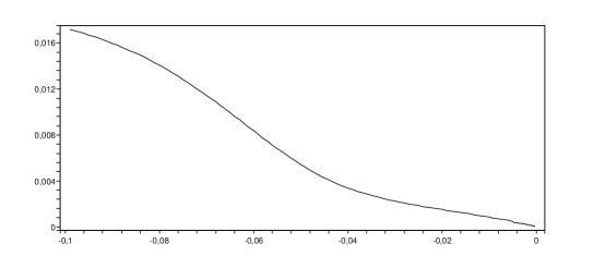
   The natural number $N$ can be chosen using the astronomers recipe. It simply chooses $N$ such that for fixed $\tau$ and $\varphi$ it minimizes $\left|\Gamma_{N+1}(\varphi)\tau^{-N-1}\right|$, that is, the least term of the formal series $\sum_{k\geq 1}\Gamma_{k}(\varphi)\tau^{-k}$ (see Figure 3).

   

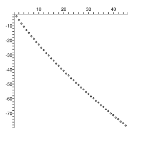
   Figure 3: Graph of $\log_{10}\left(\frac{\max_{j}\left|\Gamma_{k,j}\right|}{(350\pi)^{k}}\right)$

   .

2. A point on the unstable manifold (resp. stable manifold) can be represented in the coordinates $(\varphi,\tau)$. In order to obtain a point close to the unstable manifold we fix a positive real number $\sigma\in\mathbb{R}^{+}$ and a sufficiently large $d\in\mathbb{R}^{+}$ and define $z^{-}_{0}=\mathbf{\Gamma}_{N}(-d,-i\sigma-d)$ and a tangent vector $v^{-}_{0}=\partial_{\varphi}\mathbf{\Gamma}_{N}(-d,-i\sigma-d)$. Analogously, for the stable manifold we define $z^{+}_{0}=\mathbf{\Gamma}_{N}(d,-i\sigma+d)$ and $v^{+}_{0}=\partial_{\varphi}\mathbf{\Gamma}_{N}(d,-i\sigma+d)$.

3. The next step is to measure the difference of stable and unstable manifold at the point $(\varphi,\tau)=(0,-i\sigma)$. Taking into account the periodicity in $\varphi$ we set $d$ equal to a multiple to $2\pi$ and integrate numerically the system,

   $$\begin{array}[]{l}z^{\prime}=X_{H_{0}}(z)\\ v^{\prime}=DX_{H_{0}}(z)v\\ \end{array}$$ (39)

   forward in time with $t\in[0,d]$ and initial conditions $z^{-}(0)=z_{0}^{-},v^{-}(0)=v_{0}^{-}$ and then backward in time with $t\in[-d,0]$ and initial conditions $z^{+}(0)=z_{0}^{+},v^{+}(0)=v_{0}^{+}$.

4. Finally we evaluate,

   $$\hat{\Theta}(\sigma)=\Omega(z^{+}(-d)-z^{-}(d),v^{-}(d))e^{\sigma}$$ (40)

Remark 1.

The stable and unstable manifolds have the same asymptotic expansion, hence the difference $z^{+}(-d)-z^{-}(d)$ is exponentially small, i.e. comparable with $e^{\sigma}$. Thus the system (39) has to be integrated with great accuracy. In the case of GSHE an excellent integrator can be constructed using a high order Taylor series method.

2.2 Numerical results

In all current computations we have used a Taylor series method, which is incorporated in the Maple Software, to integrate the equations of motion (39). The method uses an adaptive step procedure controlled by a local error tolerance which was set to $10^{-D}$, where $D$ is the number of significant digits used in the computations. The order of the method has been automatically defined using the formula $\max(22,\left\lfloor 1.5D\right\rfloor)$.

Having fixed $\kappa=2$ (which we recall to be one of the parameters of the original equation (1)) we have computed the first 45 coefficients of the formal separatrix $\hat{u}_{0}$ with 60 digits precision. The error committed by the approximation $\mathbf{\Gamma}_{N}$ is approximately of the order of the first missing term.

Figure 4: The top figure represents the graph of the function $\mathrm{Im}(\hat{\Theta}(\sigma))e^{\sigma}-10.472161956944$ and the bottom figure represents the graph of the function $\mathrm{Re}(\hat{\Theta}(\sigma))e^{\sigma}$. When $\sigma$ is around 25 the rounding errors become visible and the convergence stops. The dashed curves represent the magnitude of the rounding errors.

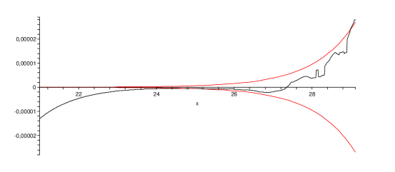
Using double precision (16 digits) we have integrated numerically the equations (39) to obtain $\hat{\Theta}(\sigma)$ for values of $\sigma$ uniformly distributed in the interval $\left[20,28.89\right]$. The initial conditions were computed using $d=350\pi$ and the first 9 terms of $\mathbf{\Gamma}_{N}$. The results are depicted in Figure 4. The expected errors are bounded by the dashed curves. This implies in particular that the method is numerically stable, that is, the propagation errors due to integration do not increase drastically. There are several sources of errors that affect the accuracy of the computation of the Stokes constant, namely:

• Approximation of stable and unstable manifolds given by the function $\mathbf{\Gamma}_{N}$;

• Errors due to the numerical integration;

• Rounding errors.

The first and the second source of errors can be made small compared to the rounding errors, which can be roughly estimated by,

$$\frac{C}{\sigma^{2}}10^{-D}e^{\sigma},$$ (41)

where $D$ is the number of digits used in the computations and $C$ is a real positive constant which reflects the propagation of rounding errors. Using this estimate we have provided bounds for the rounding errors which can be observed in Figure 4. The constant $C$ can be estimated by fitting the function (41) to the points $\left|\hat{\Theta}(\sigma)\right|$ for $\sigma\geq 25$. Using the method of least squares we have concluded that $C$ is approximately $38.5$.

With double arithmetic precision the method previously described allows the computation of 7 to 8 correct digits of the Stokes constant $\Theta_{0}$. In fact the rounding errors in computing $\hat{\Theta}(\sigma)$ from formula (40) grow accordingly to (41) whereas the neglected terms of the formula (38) decrease like $C_{1}e^{-\sigma}$, where $C_{1}$ is some positive constant. Hence the optimal is attained when both contributions are of the same order. The constant $C_{1}$ can be estimated by fitting the function $C_{0}+C_{1}e^{-\sigma}$ to the points $\left|\hat{\Theta}(\sigma)\right|$ for $\sigma\leq 24$. Using the method of least squares we have obtained that $C_{1}$ is approximately $17305.75$. Using this information we can determine the value $\sigma^{*}$ where both contributions are essentially of the same order. This means that $\sigma^{*}$ must satisfy the equation,

$$(e^{-\sigma})^{2}=\frac{C}{{\sigma}^{2}\,C_{1}}10^{-D}$$

which implies,

$$\left|\Theta_{0}-\hat{\Theta}(\sigma^{*})\right|\approx\frac{816}{\sigma^{*}}10^{-\frac{D}{2}}$$

$D$	$\sigma^{*}$	$\mathrm{Re}(\hat{\Theta}(\sigma^{*}))$	$\mathrm{Im}(\hat{\Theta}(\sigma^{*}))$
16	24.68	2.7e-05	10.47216143901571
20	29.46	7.8e-07	10.472161953423286113
24	34.21	1.6e-08	10.4721619569069446924024
28	38.95	3.1e-10	10.47216195694413924682820786
32	43.67	5.3e-12	10.472161956944396725504278408504
36	48.37	8.5e-14	10.4721619569443983419527788851129556
40	53.07	1.2e-15	10.47216195694439835812989263311456886391
44	57.76	1.8e-17	10.472161956944398358284180684468467819622191
48	62.45	2.6e-19	10.4721619569443983582855084356725900717201861670
52	67.12	3.5e-21	10.47216195694439835828552130242825730920048239485015
56	71.80	4.7e-23	10.472161956944398358285521430879142372532568396894067732
60	76.46	6.2e-25	10.4721619569443983582855214320209319731283197852962601326570
64	81.13	8.0e-27	10.47216195694439835828552143203166495538939445255794702026972749
68	85.79	1.0e-28	10.472161956944398358285521432031900047829633854060398152634432422925

Table 1: Stokes constant evaluated at the optimum $\sigma^{*}$ for different computer precisions. In the computations we have used $d=350\pi$ and $N=40$

In this way it is possible to obtain 8 correct digits for the Stokes constant using only double precision. In Table 1 we have listed the values of $\hat{\Theta}(\sigma^{*})$ evaluated at the optimum $\sigma^{*}$ for higher computer precisions. The digits in bold correspond to correct digits of the Stokes constant. We also note that the numerics suggest that $\Theta_{0}$ is pure imaginary which agrees with our prediction.

Finally, let us mention that in the process of computing the Stokes constant we have made several choices for the parameters. Namely, the number of terms $N$ used to compute $\mathbf{\Gamma}_{N}$ and the parameter $d$ which were used in computing the initial conditions of step (ii) of the numerical scheme. In fact the results are independent of these particular choices and Table 2 demonstrates the robustness of the numerical method.

$d\backslash N$	10	20	30
100$\pi$	10.47216215179386	10.47216215183208	10.47216215181955
150$\pi$	10.47216131335742	10.47216131335746	10.47216131335772
200$\pi$	10.47216144775669	10.47216144775671	10.47216144775682
250$\pi$	10.47216149546998	10.47216149546998	10.47216149547027
300$\pi$	10.47216132022817	10.47216132022820	10.47216132022773
350$\pi$	10.47216138600882	10.47216138600883	10.47216138600868

Table 2: Comparison of the value of $\mathrm{Im}(\hat{\Theta}(25))$ for different values of parameters $N$ and $d$.

3 High precision computations of an asymptotic expansion for the homoclinic invariant

In this section we present a numerical method for the computation of the homoclinic invariant as defined in (30) for the Swift-Hohenberg equation with $\kappa=2$ and $\epsilon<0$. Moreover we investigate from a numerical point of view the validity of the asymptotic expansion (37) for the homoclinic invariant. This section follows the ideas of [12] originally developed for the study of exponentially small phenomena for area-preserving maps.

In order to compute the homoclinic invariant (10) we need to compute two tangent vectors at the symmetric homoclinic point $\mathbf{\Gamma}^{s}_{\epsilon}(0,0)$. Using the fact that the system is reversible we can obtain the stable tangent vector $\partial_{\varphi}\mathbf{\Gamma}^{s}_{\epsilon}$ by applying the reversor to the unstable tangent vector $\partial_{\varphi}\mathbf{\Gamma}^{u}_{\epsilon}$. The unstable tangent vector $\partial_{\varphi}\mathbf{\Gamma}^{u}_{\epsilon}$ lives in the tangent plane of the unstable manifold at the symmetric homoclinic orbit. Thus an easy way to compute this tangent vector is to approximate the primary homoclinic orbit near the equilibrium point by the following expansion,

$$\mathbf{\Gamma}_{\epsilon,N}^{u}(\varphi,z)=\sum_{k=1}^{N}e^{kz}\left(\mathbf{c}_{k}(\epsilon)+\sum_{j\geq 1}^{k}\mathbf{a}_{k,j}(\epsilon)\cos(j\varphi)+\mathbf{b}_{k,j}(\epsilon)\sin(j\varphi)\right)$$ (42)

and then use the variational equations,

$$\begin{split}\mathbf{x}^{\prime}&=X_{H_{\epsilon}}(\mathbf{x})\\ \mathbf{v}^{\prime}&=DX_{H_{\epsilon}}(\mathbf{x})\mathbf{v}\\ \end{split}$$ (43)

to transport the tangent vector $\partial_{\varphi}\mathbf{\Gamma}_{\epsilon,N}^{u}$ along the primary homoclinic orbit until it hits the symmetric plane $\mathrm{Fix}(S)$ defined by $\left\{q_{2}=0,p_{1}=0\right\}$. Let us present the details of the method.

3.1 A method for the computation of the homoclinic invariant

1. The first step is to determine the coefficients of (42). To that end we take a new expansion,

   $$u_{N}(\varphi,z)=\sum_{k=1}^{N}e^{kz}\left(c_{k}(\epsilon)+\sum_{j\geq 1}^{k}a_{k,j}(\epsilon)\cos(j\varphi)+b_{k,j}(\epsilon)\sin(j\varphi)\right)$$

   and substitute into the equation,

   $$((\alpha_{\epsilon}\partial_{\varphi}+\beta_{\epsilon}\partial_{z})^{2}+1)^{2}\,u=\epsilon u+2u^{2}-u^{3}$$ (44)

   and collect the terms of the same order in $e^{kz}$. In this way it is possible to determine coefficients $c_{k}$, $a_{k,j}$ and $b_{k,j}$. It is not difficult to see that the coefficients $a_{1,1}$ and $b_{1,1}$ satisfy no relations and that all other coefficients depend from these two. So we define,

   $$a_{1,1}=r_{0}\cos(\psi_{0})\ \ \mathrm{and}\ \ b_{1,1}=r_{0}\sin(\psi_{0})$$

   Now recall that the first component of $\mathbf{\Gamma}^{u}_{\epsilon}$ solves equation (44) and due to the asymptotic behavior (1.4) we conclude that for $z<<0$ and $\delta<<1$ it is approximately,

   $$e^{z}\left(-\frac{2\delta}{\sqrt{\eta}}\cos(\varphi)+\frac{\delta^{2}}{\sqrt{\eta}}\left(1+\frac{2\mu}{\eta}\right)\sin(\varphi)\right)+O(e^{2z})$$ (45)

   where $\epsilon=-4\delta^{2}$. Next we ”match” the leading order of $u_{N}(\phi,s)$ with the expression (45) and conclude that $\psi_{0}$ and $r_{0}$ must satisfy,

   $$\begin{split}\psi_{0}&=\arctan\left(-\left(1+\frac{2\mu}{\eta}\right)\frac{\delta}{2}\right)\\ r_{0}&=\frac{2\delta}{\sqrt{\eta}}\sqrt{1+\left(1+\frac{2\mu}{\eta}\right)^{2}\frac{\delta^{2}}{4}}\end{split}$$ (46)

   Taking into account (4) we reconstruct $\mathbf{\Gamma}_{\epsilon,N}^{u}$ from $u_{N}$ and due to the ”matching” (46) we have,

   $$\mathbf{\Gamma}_{\epsilon}^{u}(t,t)\approx\mathbf{\Gamma}_{\epsilon,N}^{u}(t,t),\ \mathrm{as}\ \ t\rightarrow-\infty,\ \delta\rightarrow 0.$$

   That is, for small values of $\delta$, the expansion $\mathbf{\Gamma}_{\epsilon,N}^{u}$ provides a good approximation of the primary homoclinic orbit near the equilibrium point.

2. The second step is to improve the accuracy of the approximation of the symmetric homoclinic point, provided by $\mathbf{\Gamma}_{\epsilon,N}^{u}$. Given small $\delta$ and sufficiently large $T_{0}>0$ we want to determine $(T,\psi)$ such that,

   $$\mathbf{x}^{\prime} =X_{H_{\epsilon}}(\mathbf{x}), \mathbf{x}(0;\psi) =\mathbf{\Gamma}_{\epsilon,N}^{u}(-\alpha_{\epsilon}T_{0},-\beta_{\epsilon}T_{0};\psi)$$

   subject to,

   $$\mathbf{x}(T;\psi)\in\mathrm{Fix}(S)$$ (47)

   This problem can be solved using Newton method. Starting from $(T_{0},\psi_{0})$ we obtain a sequence of points $(T_{i},\psi_{i})$,

   $$\begin{pmatrix}T_{i+1}\\ \psi_{i+1}\end{pmatrix}=\begin{pmatrix}T_{i}\\ \psi_{i}\end{pmatrix}-\begin{pmatrix}\frac{\partial q_{2}}{\partial T}(T_{i};\psi_{i})&\frac{\partial q_{2}}{\partial\psi}(T_{i};\psi_{i})\\ \frac{\partial p_{1}}{\partial T}(T_{i};\psi_{i})&\frac{\partial p_{1}}{\partial\psi}(T_{i};\psi_{i})\end{pmatrix}^{-1}\begin{pmatrix}q_{2}(T_{i};\psi_{i})\\ p_{1}(T_{i};\psi_{i})\end{pmatrix}$$ (48)

   that converges to a limit $(T_{*},\psi_{*})$ such that $\mathbf{x}(T_{*};\psi_{*})\in\mathrm{Fix}(S)$, provided $(T_{0},\psi_{0})$ is sufficiently close to $(T_{*},\psi_{*})$ (see [7]). The derivatives in (48) can be computed using the variational equations along the orbit $\mathbf{x}(t;\psi)$. Later we will see that the formulae (46) provide sufficiently accurate initial guesses yielding the convergence of the Newton method.

3. Having obtained in the previous step an accurate approximation of the symmetric homoclinic point, the last step is to integrate numerically the system,

   $$\mathbf{x}^{\prime} =X_{H_{\epsilon}}(\mathbf{x}), \mathbf{x}(0;\psi) =\mathbf{\Gamma}_{\epsilon,N}^{u}(-\alpha_{\epsilon}T_{0},-\beta_{\epsilon}T_{0};\psi_{*})$$

   $$\mathbf{v}^{\prime} =DX_{H_{\epsilon}}(\mathbf{x})\mathbf{v}, \mathbf{v}(0;\psi) =\alpha_{\epsilon}\partial_{\varphi}\mathbf{\Gamma}_{\epsilon,N}^{u}(-\alpha_{\epsilon}T_{0},-\beta_{\epsilon}T_{0};\psi_{*})$$

   and evaluate the homoclinic invariant,

   $$\hat{\omega}=\Omega(\mathbf{v}(T_{*},\psi_{*}),S(\mathbf{v}(T_{*},\psi_{*})))$$

3.2 Numerical results

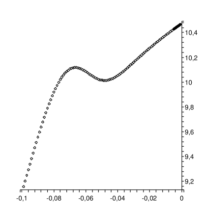
We have considered a finite set $\mathcal{I}$ consisting of points in the interval $\epsilon\in[-\frac{1}{10},-\frac{1}{1000}]$ and computed the homoclinic invariant for those points using the method previously described. For all points in $\mathcal{I}$ the magnitude of homoclinic invariant ranges from $10^{-5}$ to $10^{-45}$. Thus, in all numerical integrations we have used a high order Taylor method which allows to perform the numerical integration with very high precision. We have computed the coefficients of the expansion (42) up to $N=5$ and for each $\epsilon\in\mathcal{I}$ we have chosen $T_{0}$ sufficiently large so that $\mathbf{\Gamma}_{\epsilon,N}^{u}(-\alpha_{\epsilon}T_{0},-\beta_{\epsilon}T_{0})$ approximates the unstable manifold within the required precision. The initial point $(T_{0},\psi_{0})$ used in Newton method proved to be very close to $(T_{*},\psi_{*})$ and its relative error can be observed in Figure 5.

Figure 5: Relative error of $(T_{0},\psi_{0})$ depending on $\epsilon\in\mathcal{I}$

.

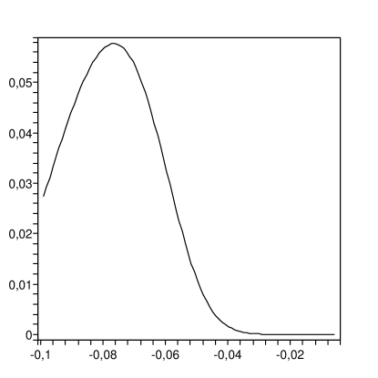
After computing the homoclinic invariant we have normalized it using the formula,

$$\bar{\omega}(\epsilon)=\frac{\omega(\epsilon)}{2}e^{\frac{\pi\alpha_{\epsilon}}{2\beta_{\epsilon}}}$$

Figure 6: Graph of the function $\bar{\omega}(\epsilon)$

.

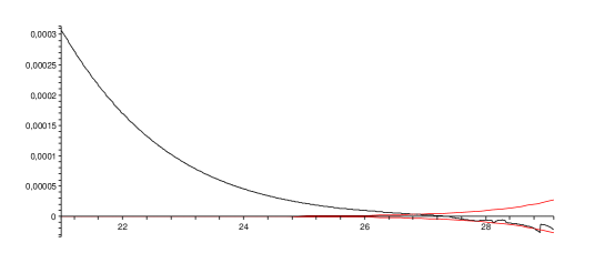
The behaviour of the function $\bar{\omega}(\epsilon)$ can be observed in Figure 6. It possible to see that it is approaching the value of the Stokes constant computed in the previous section. Moreover, it is aproaching this value in a linear fashion, supporting the validity of the asymptotic formula (6). Taking into account the asymptotic expansion for $\omega(\epsilon)$ we investigate the validity of the following asymptotic expansion for $\bar{\omega}(\epsilon)$,

$$\bar{\omega}(\epsilon)\asymp\sum_{k\geq 0}\bar{\omega}_{k}\epsilon^{k}$$ (49)

	$\bar{\omega}_{0}$	$\bar{\omega}_{1}$	$\bar{\omega}_{2}$
5	10.47216195694	8.979943127	- 42.60110
6	10.472161956944	8.979943127	- 42.601100
7	10.4721619569443	8.9799431275	- 42.6011004
8	10.47216195694439	8.97994312752	- 42.60110043
9	10.472161956944398	8.9799431275209	- 42.601100432
10	10.4721619569443983	8.9799431275210	- 42.601100432
11	10.4721619569443983	8.9799431275210	- 42.601100432
12	10.4721619569443983	8.9799431275210	- 42.6011004327
	$\bar{\omega}_{3}$	$\bar{\omega}_{4}$	$\bar{\omega}_{5}$
5	152.88	- 774.4	3.8$\times 10^{3}$
6	152.888	- 774.2	3.8$\times 10^{3}$
7	152.887	- 774.40	3.80$\times 10^{3}$
8	152.88795	- 774.39	3.814$\times 10^{3}$
9	152.88795	- 774.394	3.813$\times 10^{3}$
10	152.887958	- 774.3944	3.8138$\times 10^{3}$
11	152.887958	- 774.3944	3.813$\times 10^{3}$
12	152.887958	- 774.3944	3.813$\times 10^{3}$

Table 3: Coefficients of the estimated polynomials for different subsets of $\mathcal{P}$ and different degrees.

To that end, we have taken 14 points evenly spaced in the interval $[-2.7\times 10^{-3},-1.4\times 10^{-3}]$ and computed the corresponding normalized homoclinic invariant with more than 40 correct digits. Let us denote this set of homoclinic invariants by $\mathcal{P}$. Then, in order to get the first few coefficients of the asymptotic expansion (49) we have fitted a partial sum of the asymptotic expansion to the points of $\mathcal{P}$. Here we have used as many points as the number of unknown coefficients. Moreover, following [12] we have performed the following tests to evaluate the validity of the asymptotic expansion:

1. Interpolating different partial sums to different subsets of $\mathcal{P}$ should give essentially the same results for the coefficients.

2. The constant term of the interpolating polynomial should coincide with the value of the Stokes constant computed in the previous section.

3. The interpolating polynomial should reasonably approximate $\bar{\omega}(\epsilon)$ outside the interval $[-2.7\times 10^{-3},-1.4\times 10^{-3}]$, in the sense that it agrees with the main property of an aymptotic expansion:

   $$\left|\bar{\omega}(\epsilon)-\sum_{k\geq 0}^{n-1}\bar{\omega}_{k}\epsilon^{k}\right|\leq C\epsilon^{n},\ \forall\epsilon\in\left[\epsilon_{0},0\right)$$

   for some $C>0$ and $\epsilon_{0}<0$.

Figure 7: Relative error of the asymptotic expansion of $\bar{\omega}(\epsilon)$.

For the first test we have considered all possible subsets of $\mathcal{P}$ having only $6$ consecutive elements and interpolated these data by polynomials of degree 5. Then for each coefficient, we extracted the part of the number which is equal to all polynomials. We have repeated this process for polynomials of degree 6 up to degree 12. The results are summarized in Table 3, where it is possible to see that there is a good agreement between the coefficients of the different interpolating polynomials of different subsets of $\mathcal{P}$. We can also infer from Table 3 that the results are numerically stable. Thus, we have the following estimates for the first 6 coefficients of (49):

$$\bar{\omega}_{0} =10.4721619569443983\ldots \bar{\omega}_{1} =8.9799431275210\ldots \bar{\omega}_{2} =-42.601100432\ldots$$

$$\bar{\omega}_{3} =152.887958\ldots \bar{\omega}_{4} =-774.3944\ldots \bar{\omega}_{5} =3.813\ldots\times 10^{3}$$

Furthermore, it is clear that the coefficient $\bar{\omega}_{0}$ coincides (up to 18 digits) with the value of the Stokes constant which we recall,

$$\left|\Theta_{0}\right|=10.47216195694439835828552143203190\ldots$$

Moreover, in Figure 7 we see that the relative error of the asymptotic expansion does not exceed $0.06$ in the hole interval $\left[-\frac{1}{10},0\right]$. Thus, our numerical results provide a satisfactory numerical evidence that supports the correctness of the asymptotic expansion (37).

Appendix A Transformation of GSHE to the normal form

In order to normalize $H_{\epsilon}$ up to order $5$, we have used the method of Lie series to determine Hamiltonians $F_{i}$, $i=0,\ldots,4$ which generate the following near identity canonical map,

$$\Psi_{5}=\Phi_{F_{0}}^{1}\circ\Phi_{F_{1}}^{1}\circ\Phi_{F_{2}}^{1}\circ\Phi_{F_{3}}^{1}\circ\Phi_{F_{4}}^{1}\,,$$

where

$$\begin{split}F_{0}&=\epsilon\,\left(-{\frac{5}{32}}\,{q_{1}}\,{p_{1}}+{\frac{3}{32}}\,{q_{2}}\,{p_{2}}+\frac{1}{8}\,{p_{1}}\,{p_{2}}\right)\\ F_{1}&={\frac{7}{216}}\,\kappa\,\sqrt{2}{{q_{1}}}^{2}{p_{2}}+{\frac{95}{216}}\,\kappa\,\sqrt{2}{q_{1}}\,{q_{2}}\,{p_{1}}+{\frac{17}{72}}\,\kappa\,\sqrt{2}{q_{1}}\,{{p_{1}}}^{2}+{\frac{5}{36}}\,\kappa\,\sqrt{2}{q_{1}}\,{{p_{2}}}^{2}+\\ &\quad{\frac{175}{432}}\,\kappa\,\sqrt{2}{{q_{2}}}^{2}{p_{2}}+\frac{1}{36}\,\kappa\,\sqrt{2}{q_{2}}\,{p_{1}}\,{p_{2}}-\frac{1}{12}\,\kappa\,\sqrt{2}{{p_{1}}}^{2}{p_{2}}-\frac{1}{18}\,\kappa\,\sqrt{2}{{p_{2}}}^{3}\\ F_{2}&=\left(-{\frac{517}{20736}}\,{\kappa}^{2}+{\frac{29}{512}}\right){q_{1}}\,{{p_{1}}}^{3}+\left(-{\frac{217}{20736}}\,{\kappa}^{2}+{\frac{17}{512}}\right){q_{1}}\,{p_{1}}\,{{p_{2}}}^{2}+\\ &\quad\left({\frac{2327}{20736}}\,{\kappa}^{2}-{\frac{31}{512}}\right){q_{2}}\,{{p_{1}}}^{2}{p_{2}}+\left(-{\frac{19}{512}}+{\frac{2027}{20736}}\,{\kappa}^{2}\right){q_{2}}\,{{p_{2}}}^{3}+\\ &\quad\left(-{\frac{5}{128}}+{\frac{7}{192}}\,{\kappa}^{2}\right){{p_{1}}}^{3}{p_{2}}+\left({\frac{19}{576}}\,{\kappa}^{2}-{\frac{3}{128}}\right){p_{1}}\,{{p_{2}}}^{3}\\ F_{3}&=\epsilon\,\left(-{\frac{143}{1152}}\,\kappa\,\sqrt{2}{{p_{1}}}^{2}{p_{2}}-{\frac{167}{1728}}\,\kappa\,\sqrt{2}{{p_{2}}}^{3}\right)\\ F_{4}&=-{\frac{2}{1215}}\,\sqrt{2}\kappa\,\left(37\,{\kappa}^{2}-27\right){{p_{2}}}^{5}-{\frac{1}{648}}\,\sqrt{2}\kappa\,\left(-45+52\,{\kappa}^{2}\right){{p_{1}}}^{4}{p_{2}}-\\ &\quad{\frac{1}{243}}\,\sqrt{2}\kappa\,\left(-27+34\,{\kappa}^{2}\right){{p_{1}}}^{2}{{p_{2}}}^{3}\\ \end{split}$$ (50)

Using an algebraic manipulator it is not difficult to see that $\Psi_{5}$ transforms $H_{\epsilon}$ into the desired form.

References

- [1] I. Baldomá, The inner equation for one and a half degrees of freedom rapidly forced Hamiltonian systems, Nonlinearity, Vol. 19(6): 1415-1445, 2006.
- [2] L. A. Belyakov, L. Yu. Glebsky and L. M. Lerman, Abundance of stable stationary localized solutions to the generalized D Swift-Hohenberg equation. Computational tools of complex systems, I. Comput. Math. Appl. 34 (1997), no. 2-4, 253–266.
- [3] D. Bonheure, P. Habets and L. Sanchez, Heteroclinics for fourth order symmetric bistable equations. Atti Semin. Mat. Fis. Univ. Modena Reggio Emilia 52 (2004), no. 2, 213–227 (2005).
- [4] N. Burgoyne, R. Cushman, Normal forms for real linear hamiltonian systems with purely imaginary eigenvalues. Celestial Mechanics, 8:435–443, 1974.
- [5] J. Burke, E. Knobloch, Localized states in the generalized Swift-Hohenberg equation. Phys. Rev. E (3) 73 (2006), no. 5, 056211, 15 pp
- [6] A. R. Champneys. Homoclinic orbits in reversible systems and their applications in mechanics, fluids and optics. Physica D, 112:158–186, 1998.
- [7] A. R. Champneys and A. Spence. Hunting for homoclinic orbits in reversible systems; a shooting technique. Advances in Computational Mathematics, 1:81–108, 1993.
- [8] S. J. Chapman and G. Kozyreff, Exponential asymptotics of localised patterns and snaking bifurcation diagrams, Phys. D, Vol. 238 (3): 319-354, 2009.
- [9] J. P. Gaivão, Exponentially Small Splitting of Invariant Manifolds near a Hamiltonian-Hopf Bifurcation, Phd Thesis, University of Warwick, 2010.
- [10] Gelfreich V. A proof of the exponentially small transversality of the separatrices for the standard map, Comm. Math. Phys. 201/1, pp. 155–216, 1999.
- [11] V. Gelfreich and V. Lazutkin. Splitting of separatrices: perturbation theory and exponential smallness. Russian Math. Surveys, 56:499–558, 2001.
- [12] V. Gelfreich and C. Simó. High-precision computations of divergent asymptotic series and homoclinic phenomena. DCDS-B, 10(2/3):511–536, 2008.
- [13] L. Yu. Glebsky and L. M. Lerman. On small stationary localized solutions for the generalized 1d swift-hohenberg equation. Chaos: Internat. J. Nonlin. Sci., 5(2):424–431, 1995.
- [14] M. Haragus, A. Scheel, Interfaces between rolls in the Swift-Hohenberg equation. Int. J. Dyn. Syst. Differ. Equ. 1 (2007), no. 2, 89–97.
- [15] P. Hartman, On local homeomorphisms of Euclidean spaces. Bol. Soc. Mat. Mexicana (2), 5:220–241, 1960.
- [16] V. Hakim, K. Mallick, Exponentially small splitting of separatrices, matching in the complex plane and Borel summation. Nonlinearity, Vol. 6: 57-70, 1993.
- [17] G. Iooss and M. C. Pérouème. Perturbed homoclinic solutions in reversible 1:1 resonance vector fields. Journal of Differential Equations, 102:62–88, 1993.
- [18] J. Knobloch, T. Wagenknecht, Snaking of multiple homoclinic orbits in reversible systems. SIAM J. Appl. Dyn. Syst. 7 (2008), no. 4, 1397–1420.
- [19] L. M. Lerman and L. A. Belyakov. Stationary localized solutions, fronts and traveling fronts to the generalized Swift-Hohenberg equation. EQUADIFF 2003: Proceedings of the International Conference on Differential Equations, pages 801–806, 2003.
- [20] L. Lerman, A. Markova, On stability at the Hamiltonian Hopf Bifurcation, Regular and Chaotic Dynamics, v.14, No.1 (2009), 148-162.
- [21] Jan-Cees van der Meer, The Hamiltonian Hopf bifurcation. Lecture Notes in Mathematics, 1160. Springer-Verlag, Berlin, 1985. 115 pp
- [22] C. Olivé, D. Sauzin and T. M. Seara. Resurgence in a Hamilton-Jacobi equation. Annales de l’Institut Fourier, Vol. 53(4): 1185-1235, 2003.
- [23] A. G. Sokol’sky, On Stability of Autonomous Hamiltonian System with Two Degrees of Freedom in the Case of Equal Frequencies, Prikl. Mat. Meh., 1974, vol. 38, no. 5, pp. 791-799 [ J. Appl. Math. Mech., 1975, vol. 38, pp. 741-749]
- [24] J. Swift and P. Hohenberg. Hydrodynamic fluctuations at the convective instability. Physical Review A, 15:319–328, 1977.
- [25] D. V. Treshchev, Loss of stability in Hamiltonian systems that depend on parameters. J. Appl. Math. Mech. 56 (1992), no. 4, 492–500
- [26] P. D. Woods, A. R. Champneys, Heteroclinic tangles and homoclinic snaking in the unfolding of a degenerate reversible Hamiltonian-Hopf bifurcation. Phys. D 129 (1999), no. 3-4, 147–170