Discovery of Rotational Braking in the Magnetic Helium-Strong Star Sigma Orionis E

Abstract

We present new $U$-band photometry of the magnetic Helium-strong star $\sigma$ Ori E, obtained over 2004–2009 using the SMARTS 0.9-m telescope at Cerro Tololo Inter-American Observatory. When combined with historical measurements, these data constrain the evolution of the star’s 1$\fd$19 rotation period over the past three decades. We are able to rule out a constant period at the $p_{\rm null}=0.05\%$ level, and instead find that the data are well described ($p_{\rm null}=99.3\%$) by a period increasing linearly at a rate of 77 ms per year. This corresponds to a characteristic spin-down time of 1.34 Myr, in good agreement with theoretical predictions based on magnetohydrodynamical simulations of angular momentum loss from magnetic massive stars. We therefore conclude that the observations are consistent with $\sigma$ Ori E undergoing rotational braking due to its magnetized line-driven wind.

1. Introduction

The helium-strong star $\sigma$ Ori E (HD 37479; B2Vpe; $V=6.66$) has long been known to harbor a circumstellar magnetosphere in which plasma is trapped and forced into co-rotation by the star’s strong ($\sim 10\,{\rm kG}$) dipolar magnetic field (see, e.g., Landstreet & Borra, 1978; Groote & Hunger, 1982). This magnetosphere is largely responsible for the star’s distinctive eclipse-like dimmings, which occur when plasma clouds transit across the stellar disk twice every 1$\fd$19 rotation cycle (Townsend & Owocki, 2005). Some fraction of the star’s photometric variations likely also arise from its photospheric abundance inhomogeneities, as in other chemically peculiar stars (e.g, Mikulášek et al., 2009); but for $\sigma$ Ori E the magnetospheric contribution to the variations is dominant (Townsend, 2008).

This paper presents new $U$-band photometry of the star’s primary light minimum, obtained over four seasons spanning 2004–2009 using the SMARTS 0.9-m telescope at Cerro Tololo Inter-American Observatory (CTIO). When combined with historical measurements by Hesser et al. (1977), these new data allow a precise measurement of the star’s rotation period, and its evolution, over the past three decades.

A description of the observations, both archival and new, is provided in the following section. In §3, we discuss a procedure for accurately measuring the times $t_{\rm min}$ of primary light minimum, and then use these measurements to construct a standard observed-minus-corrected ($O-C$) diagram for the star, allowing us to assess the evolution of the star’s rotation period. We discuss and summarize our findings in §4.

2. Observations

Figure 1.— Light curves for the primary minima across the five seasons (§2); filled symbols denote those points that contribute to the minimum fitting, and open symbols those that do not. Vertical bars indicate the estimated measurement errors, and the best-fit parabolae (§3.1) are drawn as the solid curves.

2.1. 1977

Hesser et al. (1977) observed a primary light minimum of $\sigma$ Ori E on the night of 1977 January 26/27, as part of their long-term Strömgren $uvby$ monitoring of the star using the number 1 0.4-m telescope at CTIO. Their photometric data were kindly provided to us in electronic form by Prof. C. T. Bolton. No error estimates were supplied, so a measurement error $\Delta u=7\,{\rm mmag}$ is assumed for all data points — the value quoted by Hesser et al. (1976) as an upper limit on their photometric uncertainties. We do not correct for the apparent season-to-season brightening noted by Hesser et al. (1977), since this has no effect on the $t_{\rm min}$ determinations. The $u$-band light curve is plotted in Fig. 1; the accompanying $vby$ data are not shown, since they play no direct role in the period determination (however, see §3.4).

2.2. 2004

We observed a primary light minimum on the night of 2004 November 26/27, during Johnson $UBVRI$ monitoring of $\sigma$ Ori E using the Cassegrain-focus Tek 2048 CCD on the SMARTS 0.9-m telescope (see Oksala & Townsend, 2007, for the full dataset). For all $U$-band exposures (in every case, $420\,{\rm s}$ long), the Tek #1 filter (center 3575 Å, FWHM 600 Å) was used in tandem with the ND3 neutral density filter (7.5 mag attenuation). CCD frames were reduced using standard iraf tasks for bias subtraction and flat-fielding, and cosmic rays were cleaned via Laplacian edge detection (van Dokkum, 2001). The phot task of the DAOPHOT package, with an aperture radius of 10 pixels ($=3.96^{\prime\prime}$) and a sky annulus radius of 15–20 pixels, was used to perform synthetic aperture photometry. Measurement errors $\Delta U$ were estimated as the sum in quadrature of the photometric noise reported by phot, the CCD read noise, and the atmospheric scintillation noise described by the expression on p. 141 of Birney et al. (2006).

As a comparison star, we adopt the nearby ($30^{\prime\prime}$) $\sigma$ Ori D (HD 37468D; B2V; $V=6.62$) due to its color and brightness similarity; the $U_{\rm E}-U_{\rm D}$ differential light curve is plotted Fig. 1. To make an independent check on the constancy of $\sigma$ Ori D, we compare its $U$-band data against $\sigma$ Ori AB (HD 37468; O9V+B0.5V; $V=3.80$). Over the night, we find a mean difference $\overline{U_{\rm D}-U_{\rm AB}}=3.240\,{\rm mag}$ and a standard deviation $\sigma(U_{\rm D}-U_{\rm AB})=2.8\,{\rm mmag}$; the latter is consistent with the mean measurement error $\overline{\Delta(U_{\rm D}-U_{\rm AB})}=2.6\,{\rm mmag}$.

2.3. 2006

We observed a primary light minimum on the night of 2006 January 30/31. The one modification to the 0.9-m instrumental setup was the removal of the ND3 neutral density filter from the light path, thereby shortening exposure times to $2\,{\rm s}$ (with the idea of obtaining more measurements during the night). In hindsight, this was a counterproductive move. Although the proximity of $\sigma$ Ori D and $\sigma$ Ori E mean that shutter corrections are unimportant, the exposures are strongly affected by scintillation noise, especially toward the end of the night when the airmass becomes large. Moreover, $\sigma$ Ori AB is saturated in all CCD frames and cannot be used as a check star.

The observations were reduced and analyzed as before; the $U_{\rm D}-U_{\rm E}$ light curve is plotted in Fig. 1.

2.4. 2008

We observed a primary light minimum on the night of 2008 November 25/26. To obtain more-reasonable ($22-65\,{\rm s}$) exposure times than in the 2006 season, we reintroduced a neutral density filter (ND2; $5.0\,{\rm mag}$). Changes to the default telescope configuration led to the inadvertent substitution of the Tek #2 $U$-band filter (center 3570 Å, FWHM 660 Å) in place of the Tek #1 filter used previously, but this should have negligible impact on our results. Due to a further oversight, the CCD gain was adjusted from the previous setting of 3.1 e^-/ADU, to 0.6 e^-/ADU; this had the unfortunate effect of significantly elevating the readout noise.

The observations were reduced and analyzed as before; the $U_{\rm E}-U_{\rm D}$ light curve is plotted in Fig. 1. Comparison of $\sigma$ Ori D against $\sigma$ Ori AB reveals a mean $\overline{U_{\rm D}-U_{\rm AB}}=3.236\,{\rm mag}$ and a standard deviation $\sigma(U_{\rm D}-U_{\rm AB})=12\,{\rm mmag}$. The latter value is rather larger than the mean measurement error $\overline{\Delta(U_{\rm D}-U_{\rm AB})}=9.8\,{\rm mmag}$, but not overly so.

2.5. 2009

We observed a primary light minimum on the night of 2009 November 28/29. We kept the ND2 filter from the 2008 season, but reverted back to the original Tek #1 $U$-band filter, and set the CCD gain to 1.5 e^-/ADU; this led to exposure times between 130 and $250\,{\rm s}$. The observations were reduced and analyzed as before; the $U_{\rm E}-U_{\rm D}$ light curve is plotted in Fig. 1. Comparison of $\sigma$ Ori D against $\sigma$ Ori AB reveals a mean $\overline{U_{\rm D}-U_{\rm AB}}=3.224\,{\rm mag}$ and a standard deviation $\sigma(U_{\rm D}-U_{\rm AB})=4.2\,{\rm mmag}$, the latter consistent with the mean measurement error $\overline{\Delta(U_{\rm D}-U_{\rm AB})}=4.0\,{\rm mmag}$.

3. Analysis

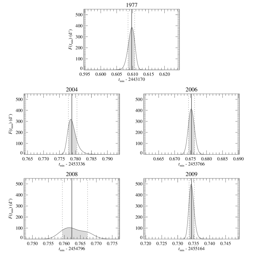
Figure 2.— Probability distribution functions for the time of primary minimum; the thick vertical line indicates the measured $t_{\rm min}$. The shaded regions to the left and right of the line each constitute 34.1% of the area under the PDF, and define the lower and upper error bounds on $t_{\rm min}$ (shown as dotted vertical lines).

3.1. Minimum Measurements

Table 1Light-curve minima from parabola fitting

Season	Band	$t_{\rm min}$ (d)	$\chi^{2}_{\rm red}$	$E$
1977	$u$	2443170.6097 ${}^{+0.0010}_{-0.0011}$	1.01	329
2004	$U$	2453336.7789 ${}^{+0.0016}_{-0.0011}$	1.56	8866
2006	$U$	2453766.6753 ${}^{+0.0010}_{-0.0009}$	1.11	9227
2008	$U$	2454796.7624 ${}^{+0.0049}_{-0.0030}$	1.12	10092
2009	$U$	2455164.7343 ${}^{+0.0009}_{-0.0007}$	0.75	10401

The determination of the time of light minimum (or maximum) in astronomical objects has received significant attention in the literature (see Sterken, 2005, and references therein). Historically the Kwee & van Woerden (1956) algorithm had long been the standard tool, but more recently polynomial fitting has emerged as a powerful and robust approach. Thus we determine the time of light minimum $t_{\rm min}$ for each of the five light curves plotted in Fig. 1 by an adaptive parabola fitting procedure:

1. The time of the dimmest point in the light curve is chosen as the initial $t_{\rm min}$.

2. Weighted $\chi^{2}$ minimization is used to fit a parabola to those points lying within 2 hours of the current $t_{\rm min}$ (this time interval is chosen to exclude the non-eclipse parts of the light curve).

3. A new $t_{\rm min}$ is chosen by analytically evaluating the minimum of the fitted parabola.

4. Steps (ii)-(iii) are repeated until the value of $t_{\rm min}$ no longer changes. (Typically, 3–4 of these iterations are required.)

The parabolic fits are drawn over the light curves in the figure, and Table 1 documents the $t_{\rm min}$ and reduced $\chi^{2}$ values associated with each fit. Here and throughout, times are expressed as heliocentric Julian dates (HJD). The tabulated $t_{\rm min}$ error bounds are calculated from bootstrap Monte Carlo simulations (Press et al., 1992). Specifically, for a given light curve comprising $n$ points, a synthetic light curve is generated by selecting $n$ points at random with replacement. The parabola fitting procedure is then used to determine $t_{\rm min}$ for the synthetic curve. This sequence is repeated many times to build up a population of synthetic $t_{\rm min}$ values, from which we derive a probability distribution function $F(t_{\rm min})$ reflecting a best estimate of the distribution from which the actual $t_{\rm min}$ measurement is drawn.

Figure 2 plots the probability distribution functions (PDFs) associated with the five $t_{\rm min}$ measurements; each is based on a population of $10^{7}$ synthetic light curves. The error bounds quoted in Table 1 are the confidence limits relative to $t_{\rm min}$ that each enclose 34.1% of the area under the PDF. Although this choice mirrors the 1-$\sigma$ limits of a Gaussian distribution, the PDFs in Fig. 2 underscore that the analysis here does not presume Gaussian errors. Moreover, while the final error in $t_{\rm min}$ is insensitive to the estimates made for the measurement errors on the individual photometric data, the Monte Carlo simulations used to derive the PDFs do properly allow the actual errors of the noisier data, e.g. in 2008, to produce a larger uncertainty in $t_{\rm min}$.

3.2. $O-C$ Fitting

Table 2Fits to the $O-C$ data

Fit Type	$b_{1}\times 10^{2}$ (d)	$b_{2}\times 10^{5}$ (d)	$b_{3}\times 10^{9}$ (d)	$p_{\rm null}$ (%)
Linear	0.38 ${}^{+0.12}_{-0.12}$	2.78 ${}^{+0.02}_{-0.01}$	–	0.05
Quadratic	1.00 ${}^{+0.12}_{-0.13}$	1.29 ${}^{+0.12}_{-0.10}$	1.44 ${}^{+0.10}_{-0.11}$	99.3

Figure 3.— The observed-minus-corrected diagram for the primary minimum measurements. The solid (dashed) lines indicate the best-fit quadratic (linear) models; the residuals relative to these models are shown below the $O-C$ diagram as filled (open) symbols.

We apply the standard $O-C$ diagram technique (e.g., Sterken, 2005) to assess the evolution of the rotation period. With the reference epoch defined by Hesser et al. (1976) and the rotation period measured by Hesser et al. (1977), an observed-minus-calculated value

$$O-C=t_{\rm min}-(2442778\fd 819+1\fd 19801E)$$ (1)

is evaluated for each $t_{\rm min}$ in Tab. 1; here and in the table, the cycle number $E$ is the integer that minimizes $|O-C|$.

Figure 3 plots $O-C$ as a function of $E$; the error bars on each point are taken from the corresponding error bounds on $t_{\rm min}$. Also shown in this $O-C$ diagram are fitted linear and quadratic models of form

$$(O-C)^{\rm mod}=b_{1}+b_{2}E$$ (2)

and

$$(O-C)^{\rm mod}=b_{1}+b_{2}E+b_{3}E^{2},$$ (3)

together with the associated fit residuals. The linear model corresponds to a constant rotation period, while the quadratic one represents a period that increases linearly with time. The coefficients $\{b_{j}\}$ are determined by a non-$\chi^{2}$ maximum likelihood estimation, which seeks to minimize the statistic

$$Q=\sum-\log F[O-C-(O-C)^{\rm mod}];$$ (4)

here, the summation is over the five light minima, each with its respective $O-C$, $(O-C)^{\rm mod}$ and $F$($t_{\rm min}$). For a given model, the quantity $\exp(-Q)$ is proportional to the likelihood that the measured $O-C$ values could have arisen by chance-fluctuation departures from the model. We use a downhill simplex algorithm (Press et al., 1992) to minimize Q, iterated until the maximum relative deviation between simplex vertices drops below $10^{-4}$.

Table 2 summarizes the coefficients $\{b_{j}\}$ of the linear and quadratic models. As in §3.1, error bounds are determined via Monte Carlo simulations. However, rather than generating synthetic $O-C$ data by bootstrapping, we construct them by perturbing each $t_{\rm min}$ with random deviates drawn from the appropriate PDF (cf. Fig. 2). From the same simulations we also determine the distribution of the Q statistic, enabling us to associate the linear and quadratic fits in Fig. 3 with a likelihood $p_{\rm null}$ (also specified in Tab. 2) that the null hypothesis is true: that is, that the deviation of the $O-C$ values from the model arises purely due to chance fluctuations.

3.3. Period Evolution

Table 2 indicates that the null hypothesis for the linear $O-C$ model is extremely unlikely ($p_{\rm null}=0.05\%$), allowing a constant rotation period to be ruled out with a high degree of confidence. However, the converse is true for the quadratic model, which fits the data extremely well. Combining its coefficients with eqns. (1) and (3) gives a revised ephemeris for the primary light minimum of $\sigma$ Ori E as

$$t_{\rm min}=2442778\fd 8290^{+0.0012}_{-0.0014}+\mbox{}\\ 1\fd 1908229^{+0.0000012}_{-0.0000010}E+1\fd 44^{+0.10}_{-0.11}\times 10^{-9}E^{2}.$$ (5)

By taking the derivative with respect to cycle number, the instantaneous period is found as

$$P=1\fd 1908229^{+0.0000012}_{-0.0000010}+2\fd 89^{+0.19}_{-0.22}\times 10^{-9}E,$$ (6)

which grows linearly at a rate $\dot{P}=77\,{\rm ms}$ per year. (We discuss the implicit assumption of smooth period growth in §4). At the reference epoch $E=0$, this period is rather larger than the $P=1\fd 19081\pm 0\fd 00001$ reported by Hesser et al. (1977); however, these authors’ error estimate seems overly optimistic. Reiners et al. (2000) determined a period $P=1\fd 19084\pm 0\fd 00001$ by combining new helium-line data with historical measurements from Pedersen & Thomsen (1977); their value is in good agreement with the mean period $\overline{P}=1\fd 190833$ obtained by averaging eqn. (6) over the 1976–1998 interval spanned by the helium data.

3.4. Systematics

Before discussing the significance of the measured period increase, we briefly review factors that may have a systematic effect on this result. As demonstrated by Townsend (2008), the timing of light minima is sensitive to the optical depth of the magnetospheric plasma clouds. In principle, the progressive shift in $t_{\rm min}$ toward later times (seen in the residuals plot of Fig. 3) could be explained by the secular accumulation of plasma in the magnetosphere (see, e.g., Townsend & Owocki, 2005). However, based on the examples given by Townsend (2008, his section 2.4), the observed shift of $\approx 0\fd 02$ between the 2004 and 2009 seasons would require a factor-six increase in the optical depth of the magnetosphere. The minima in Fig. 1 clearly do not exhibit this kind of dramatic change. Indeed, although there are some season-to-season variations in the minima depths (on the order of $20\,{\rm mmag}$), no monotonic trend is seen; we believe the variations are probably due to changes in the distribution of scattered light from $\sigma$ Ori AB. Accordingly, we rule out the possibility that the $t_{\rm min}$ shift is due to plasma accumulation.

Similar reasoning can be addressed to concerns over the change in filters, from Strömgren $u$ in 1977 to Johnson $U$ in the later observations. In passbands where the magnetosphere is more opaque, the time of primary light minimum will tend to occur later. This color-$t_{\rm min}$ correlation can be clearly seen in the Hesser et al. (1977) observations; in the Strömgren $u$ band (falling blueward of the Balmer jump), the time of primary light minimum is $0\fd 007$ later than in the $v$ band (falling redward of the Balmer jump). Because the $U$ band straddles the Balmer jump, the expected time lag between $u$ and $U$ should be around half of this, $\sim 0\fd 003$. An adjustment of this order to the 1977 $t_{\rm min}$ point, to correct for the color-$t_{\rm min}$ correlation, has a negligible effect on our results.

A final possible issue comes from the use of parabolae to measure the primary minimum times. As discussed by Sterken (2005), quadratic fitting is often eschewed in light-curve analysis on the grounds that it is unable to adequately model asymmetric light minima. However, if the shape of the light curve does not vary from cycle to cycle, then this bias is irrelevant: it matters not that $t_{\rm min}$ occurs slightly before or after the precise time of minimum, as long as the lead or lag remains invariant.

Nevertheless, to explore any bias introduced by the use of quadratic fitting, we have repeated our analysis using cubic fitting to measure the $t_{\rm min}$ values. Three salient points stand out from this re-analysis: (i) the $\chi^{2}_{\rm red}$ values of the cubic fits are not significantly smaller than those of the quadratic fits (cf. Tab. 1); (ii) there’s no evidence for a systematic lag or lead between the quadratic and cubic minima; (iii) there is an obvious difference between the widths of the PDFs, which are a factor $\sim 2$ broader in the cubic cases than in the quadratic ones. Thus, we conclude that quadratic minimum fitting does not introduce any appreciable bias, and moreover is the more robust approach.

4. Discussion

The Helium-strong star HD 37776 was found by Mikulášek et al. (2008) to exhibit a progressive lengthening in its $1\fd 5387$ rotation period, with a characteristic spin-down time $\tau_{\rm spin}\equiv P/\dot{P}=0.25\,{\rm Myr}$. For $\sigma$ Ori E the absence of photometric data in the 1980s and 1990s means that we cannot empirically differentiate between steady spin-down and a sequence of abrupt braking episodes. However, the steady scenario is lent strong support by magnetohydrodynamical (MHD) simulations of angular momentum loss in magnetically channelled line-driven winds (ud-Doula et al., 2009), which indicate that the lengthening of rotation periods should be a smooth process. Therefore, the use of a quadratic ephemeris (cf. eqn. 5) appears justified, and we derive a characteristic spin-down time $\tau_{\rm spin}=1.34^{+0.10}_{-0.09}\,{\rm Myr}$. This value coincides very well with the $\tau_{\rm spin}=1.4\,{\rm Myr}$ predicted specifically for $\sigma$ Ori E by ud-Doula et al. (2009), from their MHD-calibrated scaling law for spin-down times. (Such a close agreement is partly fortuitous, given the uncertainties in stellar and wind parameters). Assuming that $\tau_{\rm spin}$ has remained constant over the lifetime of the star implies that it can be no older than $1.16^{+0.09}_{-0.08}\,{\rm Myr}$ (otherwise, it would at some stage have been rotating faster than the critical rate $P_{\rm crit}\sim 0\fd 5$). This upper limit on the age fits within the lower portion of the $0.5-8\,{\rm Myr}$ age range estimated for the $\sigma$ Orionis cluster (Caballero, 2007, and references therein).

In summary, then, we conclude that the observations are consistent with $\sigma$ Ori E undergoing rotational braking due to its magnetized line-driven wind. This result is significant: although magnetic rotational braking is inferred from population studies of low-mass stars (e.g., Donati & Landstreet, 2009), direct measurement of spin-down in an individual (non-degenerate) object is noteworthy, and has been achieved so far for only handful of magnetic B and A stars (see Mikulášek et al., 2009).

References

- Birney et al. (2006) Birney D. S., Gonzalez G., Oesper D., 2006, Observational Astronomy, 2 edn. Cambridge University Press, New York
- Caballero (2007) Caballero J. A., 2007, A&A, 466, 917
- Donati & Landstreet (2009) Donati J., Landstreet J. D., 2009, ARA&A, 47, 333
- Groote & Hunger (1982) Groote D., Hunger K., 1982, A&A, 116, 64
- Hesser et al. (1977) Hesser J. E., Ugarte P. P., Moreno H., 1977, ApJ, 216, L31
- Hesser et al. (1976) Hesser J. E., Walborn N. R., Ugarte P. P., 1976, Nature, 262, 116
- Kwee & van Woerden (1956) Kwee K. K., van Woerden H., 1956, Bull. Astron. Inst. Netherlands, 12, 327
- Landstreet & Borra (1978) Landstreet J. D., Borra E. F., 1978, ApJ, 224, L5
- Mikulášek et al. (2009) Mikulášek Z., Szasz G., Krtička J., Zverko J., Žižåovský J., Zejda M., Gráf T., 2009, arXiv:0905.2565
- Mikulášek et al. (2008) Mikulášek Z. et al., 2008, A&A, 485, 585
- Oksala & Townsend (2007) Oksala M., Townsend R. H. D., 2007, in Okazaki A. T., Owocki S. P., Stefl S., eds, ASP. Conf. Ser. 361: Active OB-Stars: Laboratories for Stellar and Circumstellar Physics p. 476
- Olsen (1977) Olsen E. H., 1977, Information Bulletin on Variable Stars, 1332, 1
- Pedersen & Thomsen (1977) Pedersen H., Thomsen B., 1977, A&AS, 30, 11
- Press et al. (1992) Press W. H., Teukolsky S. A., Vetterling W. T., Flannery B. P., 1992, Numerical Recipes in Fortran, 2 edn. Cambridge University Press, Cambridge
- Reiners et al. (2000) Reiners A., Stahl O., Wolf B., Kaufer A., Rivinius T., 2000, A&A, 363, 585
- Sterken (2005) Sterken C., 2005, in Sterken C., ed., ASP Conf. Ser. 335: The Light-Time Effect in Astrophysics: Causes and Cures of the O-C Diagram p. 3
- Townsend (2008) Townsend R. H. D., 2008, MNRAS, 389, 559
- Townsend & Owocki (2005) Townsend R. H. D., Owocki S. P., 2005, MNRAS, 357, 251
- ud-Doula et al. (2009) ud-Doula A., Owocki S. P., Townsend R. H. D., 2009, MNRAS, 392, 1022
- van Dokkum (2001) van Dokkum P. G., 2001, PASP, 113, 1420