Coarse Graining RNA Nanostructures for Molecular Dynamics Simulations

Abstract

A series of coarse-grained models have been developed for the study of the molecular dynamics of RNA nanostructures. The models in the series have one to three beads per nucleotide and include different amounts of detailed structural information. Such a treatment allows us to reach, for the systems of thousands of nucleotides, a time scale of microseconds (i.e. by three orders of magnitude longer than in the full atomistic modelling) and thus to enable simulations of large RNA polymers in the context of bionanotechnology. We find that the 3-beads-per-nucleotide models, described by a set of just a few universal parameters, are able to describe different RNA conformations and are comparable in structural precision to the models where detailed values of the backbone P-C4’ dihedrals taken from a reference structure are included. These findings are discussed in the context of the RNA conformation classes.

Key words: RNA, Coarse Grained Modelling, Molecular Dynamics, Nanostructures

I Introduction

Recent progress in understanding RNA structure brought to light a new concept of RNA architectonics - a set of recipes for (self-)assembly of RNA nanostructures of arbitrary size and shape Jaeger and Chworos (2006); Jaeger et al. (2001). Smallest RNA building blocks - “tectoRNAs”, typically bearing well-defined structural features, such as “right angle” Jaeger and Chworos (2006), “kink-turn” Jaeger et al. (2001); Holbrook (2005) or “RNAIi/RNAIIi” Yingling and Shapiro (2007) motifs were manipulated, either experimentally Jaeger and Chworos (2006); Jaeger et al. (2001) or via a computer modelling Yingling and Shapiro (2007), into the desired 2D or 3D nanostructures (squares, hexagons, cubes, tetrahedrons etc.) that can be further assembled into periodic or quasi-periodic patterns. Compared to DNA nanostructures, RNA as a nano-engineering material brings additional challenging features, such as much larger diversity in tertiary structural building blocks [$\sim 200$ versus $\sim 20$ for DNA Jaeger et al. (2001)] and, often, increased conformational flexibility [see e.g. Sponer and Lankas (2006), p. 320]. Most useful insights about the behavior of the above-mentioned nanostructures can be gained by all-atom Molecular Dynamics (MD) simulations Sponer and Lankas (2006). However, presently, the time scales that can be achieved in the all-atom MD amount to a few (tens) nanoseconds only, which is by many orders of magnitude less than the duration of the slowest processes occurring in biomolecules (micro- to milli- to seconds). For example, in a recent study Paliy et al. (2009), we analyzed, via all-atom MD simulation, a simple RNA nanostructure of about 13 nm in size (330 nucleotides), a hexagon-shaped RNA ring Yingling and Shapiro (2007), termed “nanoring” in what follows. It is composed (1) of six RNAIi/RNAIIi complexes, which make up its sides, type A double helices, joined by the “kissing loop” motifs at the corners (e.g. AACCAUC septaloop is paired with UUGGUAG loop).  2 shows the patterns of base pairing and stacking in the kissing loops.

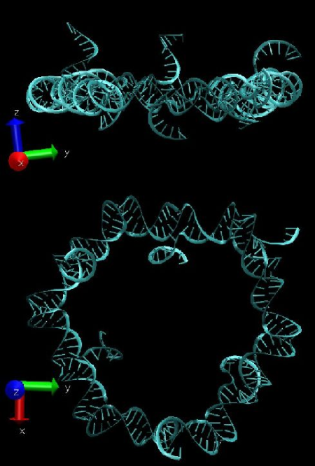
Figure 1: Side and top views of the RNA nanoring structure in the “new cartoon” representation of VMD.

In order to reach at least microsecond time scales in simulations of such nanostructures (hundreds to thousands nucleotides in size), one needs to consider a coarse-grained (CG) treatment, where the groups of atoms are represented by the CG interactions centres - “beads”, and effective interactions between such beads are set in a way to fit the nanostructures atomic connectivity, thermal, mechanical properties etc. Two kinds of data are often used in the fitting process: (i) the experimentally available structural information as well as other known properties of interest (which can be limited and/or incomplete), and (ii) a host of very detailed atomistic data obtained from all-atom MD simulations. Namely, the parameters for a CG model can be derived from both experimental and full-atom MD data by Boltzmann Inversion (BI) Reith et al. (2003) of the Radial Distribution Functions (RDFs), using the Inverse Monte Carlo scheme Lyubartsev and Laaksonen (1995) or, in the case of all-atom MD simulation only, with the “Force Matching” method Ercolessi and Adams (1994) [for some recent approaches to biomolecules, see e.g. Voth (2009); Izvekov and Voth (2005); Noid et al. (2008, 2008); Tozzini (2005); Trovato and Tozzini (2008)]. Finally, such a CG model can be further investigated using Coarse-Grained Molecular Dynamics (CGMD), which allows one to reach much longer time scales [although the dynamics of the original system is not always adequately represented Izvekov and Voth (2005)]. The main challenge is to describe the RNA on a coarse-grained level with just a few universal parameters, thus adopting the strategy of a “CG forcefield” (FF). This proved to be a difficult task, in particular in the sense of transferability of such a CG model to other structures, not used in the fitting. Transferability problems are notorius even for condensed matter, and it is even more true for the biomolecules, that show enormous structural diversity, see e.g. Voth (2009); Ouldridge et al. (2009); Ghosh and Faller (2007); Nielsen et al. (2004). In the latter case, instead of a FF approach, a lot of detailed structural information (such as equilibrium values of bonds, angles, dihedrals, nonbonded interatomic distances from the experimentally resolved structures) is supplied to the CG model, thus providing its structural precision, although in describing a given structure only. Such a structurally biased approach is often termed the Self Organized Polymer, SOP Hyeon and Thirumalai (2005).

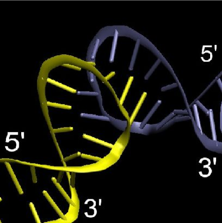
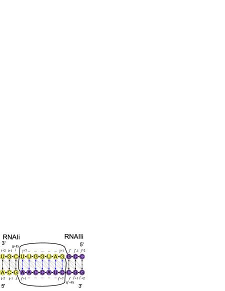
Figure 2: Top: The “new cartoon” 3D representation of one kissing loop corner of the RNA nanoring illustrating the base pairing and stacking. Bottom: 2D secondary structure sketch of the same kissing loop (colors correspond to the 3D view above); the main base pair bonds are denoted with the arrows (black in the double-helical stems, blue in the kissing loop); two auxiliary bonds (Eq. 3) per base pair are shown with gray dashed lines; the indexing scheme used in the simulation is shown; the base pairs are ordered in the sense of stacking, that occurs continuously troughout the kissing loop; two long stretched lines connecting consecutive nucleotides correspond to two sharp kinks of the nucleic backbones visible in the 3D view above.

In the CG modelling of RNA, several recent advances should be mentioned (see e.g. Hyeon and Thirumalai (2007); Hyeon et al. (2006); Hyeon and Thirumalai (2005); Trylska et al. (2005); Jonikas et al. (2009); Pincus et al. (2008); CAO and CHEN (2005); Cao and Chen (2009); Tan et al. (2006); Das and Baker (2007); Parisien and Major (2008); Ding et al. (2008); Gherghe et al. (2009)). Besides, many of the RNA modelling approaches focusing on the 3D tertiary structure prediction [reviewed in Shapiro et al. (2007)] make use of some coarse-graining via variety of methods, such as building complex CG energy functions and use of pre-compiled databases of known motifs. However, comparatively few of them are able to produce long-time dynamics once the 3D structure is known. Existing CG models for RNA, similar to those for DNA Knotts et al. (2007); Sambriski et al. (2009); Ouldridge et al. (2009), include one to three coarse grained units (beads) per nucleotide. One-bead RNA models normally use the SOP approach to achieve the desired structural precision Hyeon and Thirumalai (2007); Hyeon et al. (2006); Trylska et al. (2005); Jonikas et al. (2009) [recent model developed in Jonikas et al. (2009) uses special bonds to fix the tertiary contacts only]. On the other hand, the most recent three-bead RNA CG model Ding et al. (2008); Gherghe et al. (2009) achieves a reasonable success in structural precision (for up 100-nucleotide chains) even with a CG FF approach, that includes complex sequence-dependent interaction details and many-body treatment of the stacking, base-pairing and hydrophobic interactions [for some larger structures, it still needs the special artificially introduced bonds to fix long-range tertiary contacts Gherghe et al. (2009)]. However, the technique employed to simulate the evolution of the system, Discrete Molecular Dynamics Ding et al. (2008), while providing a means for fast folding, at the same time necessarily dictates the use of simplified step-wise potentials, which may introduce additional sources of imprecision into the model. By contrast, we use continuous potentials to describe the energetics of RNA, which should make the dynamics of the system more realistic. To put our RNA CG modelling efforts better in the perspective of the previous studies, we focus on the development of a simplest continuous CG energy function, that enables us to do long-time CGMD simulations of the huge aggregates such as RNA nanostructures (this simplicity comes at an expense - e.g. presently the secondary stucture should be known to our models, a requirement that will be lifted in the future).

Namely, in the present paper we explore the avenues from the SOP approach to a RNA CG forcefield approach by varying number of beads and amount of atomistic structural information in our series of models. We show that the inclusion of just the dihedral pseudo angles P-C4’ in a SOP manner brings about the same structural precision to the model, as the full SOP approach. Besides, a simple modification of the dihedral angle terms to allow an alternative value of each dihedral can render even the RNA FF model sufficiently precise to describe the studied RNA nanoring. These findings are consistent with the existence of the RNA conformation classes, based on P-C4’ dihedrals Wadley et al. (2007).

II Coarse-Grained Model

The development of a CG model consists of two major stages: (i) choice of the groups of atoms to be combined in a single CG bead, and (ii) selection of the functional forms and fitting of the parameters for the effective interactions between the beads.

In the case of nucleic acids, the simplest choice for stage (i) is one bead per nucleotide (beads being placed normally on the phosphate groups) which allows one to use experimentally available structural data Trylska et al. (2005); Trovato and Tozzini (2008); Jonikas et al. (2009). However, as it has been recently shown in Wadley et al. (2007), the available experimentally RNA conformations may be described well by just two torsional angles, between the P and C4’ atoms. Connecting the beads placed at the C4’ atomic sites with the base pairing bonds is not suitable in terms of the geometry, as such bonds are too far off the axis of the double helix. Instead, we adopt a representation with three beads per nucleotide, that corresponds to the (P)hosphate, (S)ugar, and nucleic (B)ase, respectively, which is a natural choice for nucleic acids. It has already been used in a few recent articles both on DNA Knotts et al. (2007); Sambriski et al. (2009) and on RNA Ding et al. (2008); Gherghe et al. (2009); Cao and Chen (2009). Note that to exploit the idea of RNA conformation classes we chose to place beads on the existing atoms rather then on the center of masses of groups of atoms.

The sample configurations of the RNA nanoring in on the one- and three-bead variants of our models (denoted as 1B and 3B in what follows) are depicted in the 3. In the 1B case, all beads of the single type (with the mass $m^{(P)}=321.5$ a.m.u.) are placed on the P atoms in the phosphates. In the 3B case, two types of beads are thus placed on the P atoms and C4’ carbons, while a number of plausible choices are possible for the placement of the third base bead. We found the following variant to be most convenient: N9 atom of purines and N1 atom of pyrimidines. The masses of the beads in the 3B representation are taken as $m^{(P)}=109$ a.m.u. , $m^{(S)}=120$ a.m.u., $m^{(B)}=92.5$ a.m.u.

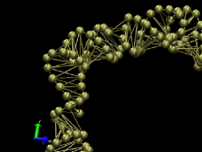
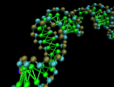
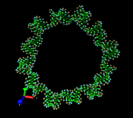
Figure 3: CG representations for the RNA nanoring shown in Fig.1. From top to bottom: Zoomed views of one ”kissing loop” in 1B and 3B representations, and the full RNA nanoring in the 3B representation. The phosphate (P) beads are shown in brown, the sugar (S) beads - in cyan, the base beads (B) - in green. The bonding of the backbone and between the bases is shown with the lines.

In our model, the beads are organised into several single chains, that correspond to the basic building blocks of the studied nanostructure, and the connectivity inside which is never broken in the course of simulation. For example, the nanoring from 1 is built up from six chains that form the sides of a hexagon, and are folded into double helical stems with septaloops at both ends. Dangling 5’ and 3’ ends of the chains, found in the middle of the hexagon sides, are excluded from the CG model in order to focus on the core of the nanoring (264 nucleotides). The total interaction energy has the following form:

$$V=V_{conn}+V_{bp}+V_{nb},$$ (1)

with the standard chain connectivity contribution $V_{conn}$:

$$V_{conn}=\sum_{chains}\left(\sum_{bonds}V_{b}(r-r^{(0)})+\sum_{angles}V_{a}(\theta-\theta^{(0)})+\sum_{dihedrals}V_{d}(\phi-\phi^{(0)})\right),$$ (2)

where $V_{b}(r)$, $V_{a}(\theta)$, $V_{d}(\phi)$ are intra-chain terms that correspond to the energies of bonds, angles, and dihedrals (often abbreviated “b/a/d” in what follows), while $r^{(0)}$, $\theta^{(0)}$, $\phi^{(0)}$ are the equilibrium values for b/a/d, respectively.

The energy term $V_{bp}$ accounts for the interactions between the base pairs. In the case of the nanoring, these include the contributions from the base pairs found inside the double-helical part of a single chain, as well as between those septuplets of the base pairs belonging to different chains, that form the kissing loops. Following the idea of Trovato and Tozzini (2008), we express the base pair interactions with three bonds per base pair instead of one:

$$V_{bp}=\sum_{i,j\in(basepairs)}U_{i,j}(r_{i,j}-r^{(0)}_{i,j})+U_{i+1,j}(r_{i+1,j}-r^{(0)}_{i+1,j})+U_{i+2,j}(r_{i+2,j}-r^{(0)}_{i+2,j}),$$ (3)

which lets us enhance structural accuracy, since it takes into account both the hydrogen bonding between bases and the stacking interactions. As illustrated in 2 (bottom, arrows and gray dashed lines), a base $j$ interacts not only with its counterpart $i$, but also with the neighboring bases $i+1$, and $i+2$ from the anti-sense part of the same double-helical stem (if present). A special care is required for laying out the base pair interactions in the kissing loops. Since a base paired kissing loop section closely resembles the double-helical structure, and the stacking occurs continuously from one stem helix through the loop -loop helix to the other stem helix Lee and Crothers (1998), in the RNA nanoring all the bases have three interacting neighbours (possibly from two different chains). The connectivity between the base pairs is thus maintained throughout the time evolution.

The remaining energy contribution $V_{nb}$ corresponds to the interactions between all bead pairs not involved in the bonded interactions described above. It has the following form:

$$V_{nb}=\sum_{i,j\in(nonbonded)}v(r_{ij}).$$ (4)

In the present paper we take the simplest Weeks-Chandler-Andersen (WCA) form Weeks et al. (1971) for the nonbonded potential $v(r)$. It consists of the repulsive part of the Lennard-Jones potential, and expresses the steric repulsion between the beads via energy $\varepsilon$ and bead diameter $\sigma$.

The MD for the CG model is implemented via the DL_POLY $2.19$ package Smith et al. (2002). The resulting CG model is relaxed via an energy minimization (conjugate gradient method) and then equilibrated at a constant temperature in the NVT ensemble [Evans algorithm, Evans and Morris (1984)] with open boundary conditions and the time step of $0.01$ ps, sufficiently small to conserve the energy of the system in the constant energy runs. The cutoff of $10$ Å  is applied to nonbonded interactions. Visualization and data processing of both all-atom MD and CGMD simulations are carried with VMD Humphrey et al. (1996), using in-house developed scripts.

III Fitting of the CG Parameters

The total energy of the CG model, Eq. 1 thus contains a number of parameters for the b/a/d, base pair terms (as well as those for the nonbonded interactions). Our general approach to the fitting of these parameters is the following: (i) the histograms of the values of various bonds, angles and dihedrals, as well as the Radial Distribution Functions (RDF) between all sorts of beads are extracted from all-atom MD trajectories; (ii) these distributions are used to fit the CG model parameters via the Boltzmann Inversion method Reith et al. (2003). Namely, given a probability distribution function $P(q)$ for a degree of freedom $q$, the corresponding potential of mean force (PMF) $V_{eff}(q)$ is determined via the following formula:

$$V_{eff}(q)=-k_{B}T\ln(P(q)).$$ (5)

Note that thus obtained $V_{eff}(q)$ coincides with the true potential energy only for the case of a single degree of freedom $q$, and generally it can serve only as a first approximation used in a subsequent iterative procedure, which may not always be successful, because many variables have to be fitted simultaneously. Fortunately, different energy contributions usually show a certain hierarchy, which allows their refinement in succession, in order of their decreasing strength, e.g. $V_{bond}\rightarrow V_{angle}\rightarrow V_{van-der-Waals}\rightarrow V_{dihedral}$ Reith et al. (2003).

We fit the effective potentials for the bonded degrees of freedom $V_{eff}(q)$, Eq. (5), by their Taylor expansions (up to quartic) around their global minima:

$$V_{eff}(q)=\frac{k}{2}(q-q^{(0)})^{2}+\frac{k^{\prime}}{3}(q-q^{(0)})^{3}+\frac{k^{\prime\prime}}{4}(q-q^{(0)})^{4}.$$ (6)

We thus obtain an equilibrium value $q^{(0)}$ of a bonded degree of freedom $q$ and the coefficients $k$, $k^{\prime}$, $k^{\prime\prime}$. For the 1B CG model, we used all three terms, while for the 3B CG model the use of only the harmonic term $k$ proved to be sufficient for our purposes (for the latter case, we made some tests with the anharmonic coefficients $k^{\prime}$ $k^{\prime\prime}$ included, and found no important differences; they may be useful in the future, for the fitting of the CG model to the dynamical properties, such as diffusivity). We find that for most of the bonded degrees of freedom (in the 3B case) the initial values of the parameters obtained directly from the Eqs. (5) and (6), already reproduce sufficiently well the histograms in the CGMD simulations, so that only seldom subsequent adjustments are required. They are done by manually introducing small changes to the coefficients in Eq. 6, in order to improve matching between the MD and CGMD distributions. For further refinement of the model, we plan to resort also to a more systematic fitting procedure, involving the iterative procedures and Force Matching method Ercolessi and Adams (1994) with cubic spline potentials Izvekov and Voth (2005) in particular.

We used two all-atom MD data sources: (i) a $6$ ns $300$ K trajectory of a simple RNA double A-helix dodecamer (GCGCUUAAGCGC); (ii) a $2$ ns $310$ K trajectory of a complex RNA nanostructure - nanoring. Both systems have been simulated in the explicit water with Mg and Na counter ions. Further details about these MD runs can be found in the Supporting Information. While the data derived from the dodecamer served us as a source for “double-helical” parameters (due to a longer trajectory they are also more reliable), the set of data derived from the nanoring, allowed us to introduce “non-helicity” into the model in a controllable manner.

It is important to stress that, for the RNA nanoring, the above-mentioned degrees of freedom are not distributed according to Boltzmann statistics only, but their distributions also reflect the spatial inhomogeneity of the system. Therefore, an attempt to represent such a degree of freedom via a single potential function using the BI method would lead to instability of the desired structure in the CG model, because such a degree of freedom would be discriminated against energetically in certain regions. Instead, one may introduce some local modifications to the potential functions. The ultimate strategy of this sort is the SOP approach, where each instance of such a degree of freedom has its own equilibrium value depending on its location in the molecule.

Thus, we consider three different parameter sets: (i) “SOP” parameter set, where the coefficients $k$, $k^{\prime}$, $k^{\prime\prime}$ of the potential functions $V_{eff}(q)$ are uniform throughout the system, while the equilibrium values $q^{(0)}$ are unique for each instance of the b/a/d; (ii) “SOP-dihedrals”, where the SOP approach (i) is applied only to the dihedrals of the nucleic acid backbone, but not to the bonds, base pairing bonds or angles, and (iii) “forcefield” (FF) parameter set where each instance of a degree of freedom is described by all uniform parameters (including their equilibrium values) throughout the system. In all cases, for the uniform part, we used the CG parameters $k$, $k^{\prime}$, $k^{\prime\prime}$, and $q^{(0)}$ extracted from the dodecamer data. However, for the SOP and the SOP-dihedrals parameters sets, we replaced the uniform equilibrium values with the full (inhomogeneous) sets found either in the initial non-equilibrated structure of the nanoring (we term such configuration “ini1” in what follows), or by the averaging of each instance of an equilibrium value over the all-atom MD trajectory of the nanoring (“ini2”).

IV Results

IV.1 1B representation of the Coarse-Grained Model

The simplest 1B representation of the model includes the following CG degrees of freedom: $(P_{i}P_{i+1})$ backbone bonds, $(P_{i}P_{i+1}P_{i+2})$ backbone angles and $(P_{i}P_{i+1}P_{i+2}P_{i+3})$ backbone dihedrals, three base-pairing bonds $(P_{i}P_{j})$ , $(P_{i+1}P_{j})$, $(P_{i+2}P_{j})$ per ($i,j$) base pair, as well as the distances for the nonbonded $(PP)$ pairs. The indices $i$ and $j$ denote the nucleotide numbers in the sequence (counting from the 5’ end), and they are omitted in what follows wherever possible without the loss of clarity.

The histograms of the backbone angles as well as RDFs for the nonbonded pairs from all-atom MD data are plotted in 4 for both the RNA dodecamer and the RNA nanoring in comparison (data for all the 1B CG degrees of freedom can be found in the Supporting Information, Fig. S1). The distributions for the RNA nanoring are in general broader, they contain extended tails, that reflect the existence of nonhelical regions. While the distribution of the backbone and base pair bond lengths are more simple and unimodal, for both the dodecamer and the nanoring, the remaining distributions (angles, dihedrals, and nonbonded pairs) for the nanoring show a number of fine features, absent in the dodecamer, and taking into account of which is crucial for the development of a CG model. Namely, the angular distributions for the nanoring show additional small peaks at $\approx 60^{\circ}$ and $\approx 110^{\circ}$ besides the main peak at $155^{\circ}$, the dihedrals show additional broad peak at $\approx-160^{\circ}$ besides the main peak at $14.4^{\circ}$, and the nonbonded RDF shows a small peak at $\approx 5$ Å  due to the closely spaced phosphates. As close examination of the atomic configurations reveals, these features are associated mostly with the regions of the kissing loops.

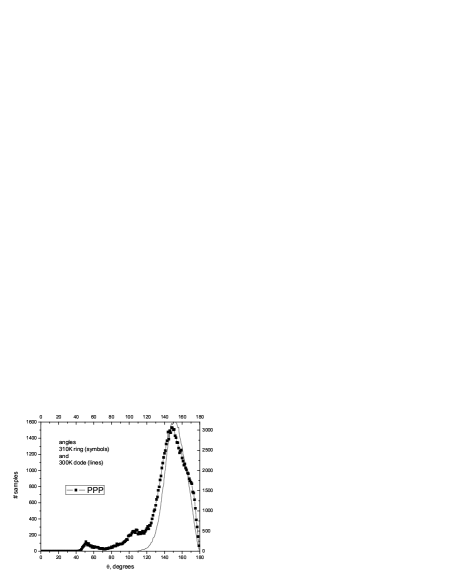
Figure 4: Angle histograms and nonbonded RDFs from all-atom MD runs for the 1B representation of the model. The data for the RNA nanoring are shown with symbols, while those for the RNA dodecamer are shown with thin lines.

Since it does not make sense to fit multi-modal distributions of the bonded CG degrees of freedom with simple potentials of Eq. (6), in the 1B variant of the model we considered only SOP parameters sets with the coefficients $k$, $k^{\prime}$, $k^{\prime\prime}$ derived from the dodecamer data. Besides, as the peak of the nonbonded RDF at $\approx 5$ Å dictates that the nonbonded interaction potential does not discriminate such small interbead spacings energetically, we have taken the values $\varepsilon=0.1$ kcal/mol, $\sigma=5.0$ Å  for the nonbonded WCA parameters. Table S1 lists the working values of the parameters for the 1B CG model. We subjected the resulting 1B CG representation of the RNA nanoring to $500$ ns equilibration at $T=300$ K. Various distributions from these equilibration runs are plotted in Fig. S2 together with the analogous all-atom MD data for comparison. While a more detailed account can be found in the Supporting Information, here we emphasize the main result - the 1B CG model fails to reproduce the overall shape of the nanoring, which collapses to various unrealistic configurations, characterized by the abundance of too closely spaced nonbonded beads, Fig. S2. This is the consequence of the above-mentioned $\approx 5$ Å restriction on the repulsive nonbonded potential (while the all-atom MD nonbonded RDFs suggest that the beads should be at least $\approx 10-15$ Å in diameter). It is possible to introduce a more complex nonbonded pair potential, with multiple minima. However, this opens a number of questions about the relative depths of the minima/heights of the barriers and the existence of unrealistic spurious configurations in the result. While a complex pair potential can be represented with splines and adjusted in a very detailed manner Izvekov and Voth (2005), this does not secure us from the latter caveat. Besides, for the FF parameter set in the 1B representation, one needs to introduce the angular and dihedral terms of the fairly complex shapes too. This combination of factors led us to abandon the 1B representation as unsuitable in favour of the 3B representation.

IV.2 3B representation of the Coarse-Grained Model

The full list of different energy terms for the 3B representation of the CG model includes the following (the layout of the bonding terms is shown in 2 and 3). Along the nucleic acid backbone the $(P_{i}S_{i})$, $(S_{i}P_{i+1})$, $(S_{i}B_{i})$ bonds between the nearest neighbours, as well as $(P_{i}S_{i}P_{i+1})$, $(S_{i}P_{i+1}S_{i+1})$, $(P_{i}S_{i}B_{i})$, $(B_{i}S_{i}P_{i+1})$ angles, $(P_{i}S_{i}P_{i+1}S_{i+1})$ and $(S_{i}P_{i+1}S_{i+1}P_{i+2})$ dihedrals are included. Along the base-paired parts of double helices and kissing loops the $(B_{i}B_{j})$ , $(B_{i+1}B_{j})$, and $(B_{i+2}B_{j})$ bonds are included. Besides, due to the topology of the 3-bead nucleic backbone, we introduce dummy “zero energy” bonds between the nearest $(S_{i}B_{i+1})$, $(B_{i}S_{i+1})$, and $(B_{i}B_{i+1})$ neighbours along the backbone in order to exclude thems from the nonbonded interactions, since these bonds are already restrained by the above-mentioned set of backbone terms.

Our 3B model includes also 6 different non-bonded bead pairings $(PP)$, $(PS)$, $(PB)$, $(SS)$, $(SB)$, and $(BB)$. The RDFs from the all-atom MD runs for three selected pair types are shown in 5 for both studied systems (the full set of data for all nonbonded as well as bonded degrees of freedom can be found in Figs. S3-S4). The nonbonded RDFs for the RNA nanoring (5) show well pronounced peaks/tails in the interval between $5$ Å and $10$ Å, which are absent in the case of the dodecamer. As in the 1B case, these features, caused by closely spaced beads in the kissing loops, dictate the choice of the same nonbonded parameters, $\varepsilon=0.1$ kcal/mol, $\sigma=5.0$ Å.

The 3B bonded distributions for the RNA nanoring show much less pronounced fine features, compared to the analogous plots for the 1B case. In fact, all the bonded terms (except the dihedrals) have unimodal distributions closely resembling Gaussians, which allows us to retain the harmonic coefficients $k$ only in Eq. 6. More complex distributions are demonstrated by the dihedral angles. They are plotted in 5 for both the RNA nanoring and the RNA dodecamer for comparison. For example, the (PSPS) dihedrals contain two shoulders near the main peak at $\approx-153.4^{\circ}$ consistent with two RNA conformational classes Wadley et al. (2007), as further explained in the Discussion.

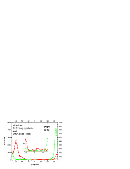
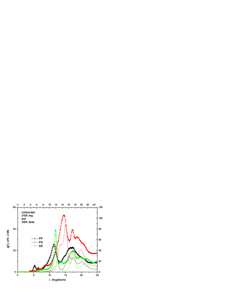
Figure 5: Top: Histograms for dihedral angles from all-atom MD runs in the 3B representation of the model. The inset shows the zoomed portion of the figure near the baseline in the interval $[-100^{\circ},140^{\circ}]$. Bottom: Radial Distribution Functions for nonbonded interactions from all-atom MD runs for the 3B representation of the model. The data for the RNA nanoring are shown with symbols, while those for the RNA dodecamer are shown with thin lines (the color coding is the same in both cases).

Besides, as more careful examination of the dihedral histograms for both (PSPS) and (SPSP) reveals, there exist some dihedral values (mainly in the kissing loops), that deviate strongly from the centres of the distributions (inset in 5). Their fraction is not high, however their presence has to be taken into account in a CG model. The detailed dependences of the (PSPS) and (SPSP) dihedrals along the ring versus the dihedral index for ini2 SOP parameter set are shown in 6 (Fig. S5 show similar plots for ini1). In both cases, the dihedrals deviating by $\sim 180^{\circ}$ (we term them cis) from the distribution centres are clearly visible (the latter correspond approximately to the trans orientation). They belong to the 12 localized parts of the nucleic acid backbones (the sharp backbone kinks in 2) participating in 6 kissing loops, i.e. in total there are four such outstanding cis dihedrals per kissing loop pair. In the FF variant of the model, where all the dihedrals of the same type should have the same uniform equilibrium value, such dihedrals would be strongly discriminated against energetically by a harmonic or a quartic effective potential of Eq. 6, and this would strongly distort the equilibrium structure of the kissing loops. As a remedy, we tested the following dihedral function:

$$V_{eff}(\phi)=\frac{k}{4}[1-\cos(2(\phi-\phi_{0}))],$$ (7)

that has two minima at $\phi=\phi_{0}$ and $\phi=\phi_{0}+180^{\circ}$, both with stiffness $k$. It turns out that by accommodating the cis dihedrals, this simple function provides an excellent performance for the FF variant of the model in describing the RNA nanoring.

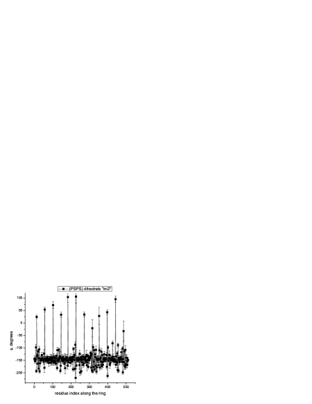
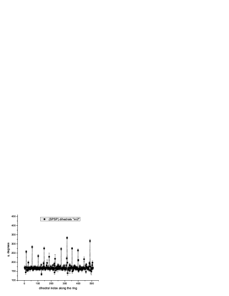
Figure 6: The ”SOP” fields of the dihedral angles introduced in the 3B model. Top: for initial configuration termed ”ini1”. Bottom: averaged over a all-atom MD trajectory (termed ”ini2”). To represent better the deviating dihedrals, the plotting intervals are chosen as follows: PSPS dihedrals are shown within $[-240^{\circ},120^{\circ}]$, SPSP dihedrals are shown within $[0^{\circ},360^{\circ}]$.

Since we intended to describe the RNA nanoring with a simple CG model based on the main body of purely helical parameters, with a controlled amount of non-helicity introduced either via SOP or via a FF with cosine dihedral term, we have chosen the set of bonded parameters fitted via the BI method from the RNA dodecamer data, and tested it on the RNA nanoring. The 1 lists the values of parameters for the 3B CG model we thus obtained. To compare the performance of all the considered six variants of the 3B CG model, namely the SOP, SOP-dihedrals (both with ini1 and ini2 detailed sets) as well as two FF variants with the harmonic Eq. 6 (termed ”FF–harmonic”) and cosine Eq. 7 (“FF–cosine–dihedrals”) dihedral functions, we performed a series of $750$ ns long CGMD equilibration runs at constant temperature of $300$ K. The dihedral histograms and RDFs for nonbonded (PP) pairs obtained by the end of these runs are shown in 7 and 8, respectively, in comparison to the distributions from all-atom MD (full set of data can be found in the Figs. S6-S10). After a few minor manual adjustments of the CG parameters, the histograms of the bonded terms show reasonable agreement with those from the all-atom MD simulations (apart from some non-essential discrepancies further discussed in the remarks in Supporting Information). The dihedral distributions show the required extended tails in all cases except, obviously, FF–harmonic (7, the insets). What is even more remarkable, all the variants of the CG model (except the FF–harmonic) are able to capture the fine features of the nonbonded RDFs. The most important of them is the $5$ Å peak for the $PP$ pairs (8), which is even slightly over-emphasized by the FF–cosine–dihedrals variant.

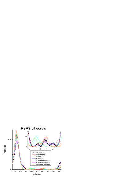
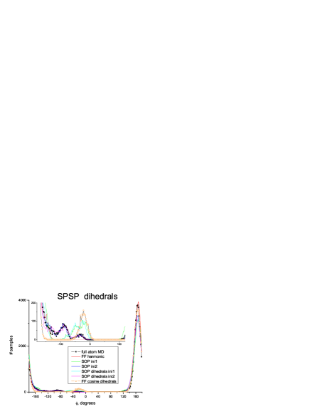
Figure 7: Dihedrals histograms for RNA nanoring from full atom MD and from CGMD runs for comparison. The insets show the zoomed portions near the baselines in the interval $[-100^{\circ},160^{\circ}]$ (PSPS) and $[-180^{\circ},120^{\circ}]$ (SPSP), respectively. The small peaks near the baselines are reproduced equally well by SOP and SOP-dihedrals variants of the CG model, and they are also reasonably reproduced by FF-cosine-dihedrals variant, as further discussed in the text.

The Root Mean Square Deviations (RMSDs) from the initial structures during these runs are plotted in 9. Typical values of RMSD are $13.0\pm 3.0$ Å for SOP ini1 and ini2, $13.5\pm 3.5$ Å for SOP–dihedrals ini1 and ini2, and the RMSD is about the same ($16.1\pm 3.2$ Å) for the FF–cosine–dihedrals variant. These values are to be compared to the typical values for the dodecamer (also plotted in 9 $4.5\pm 1.5$ Å for all considered variants) and to $35\pm 5.0$ Å for the FF–harmonic variant for the nanoring (not plotted) in which case the overall shape of the nanoring is not preserved. The final snapshots of the nanoring for the SOP–dihedrals and FF–cosine–dihedrals variants are depicted in the same figure, attesting to the preservation of the helical segments, kissing loop structures and the overall shape.

We conclude therefore, that the 3B CG model provides an excellent description for the structurally inhomogeneous RNA aggregate - the nanoring. This shows the power of the 3B representation, which, unlike the 1B one, captures adequately the excluded volume effects with small ($\approx 5$ Å in size) beads while allowing for closely spaced beads in the kissing loops.

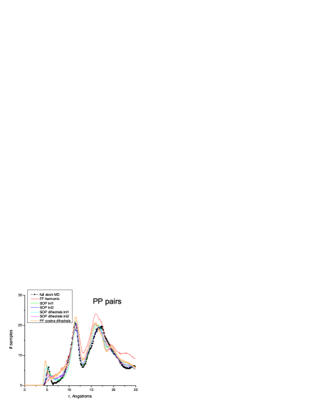
Figure 8: RDFs for nonbonded $PP$ pairs for the RNA nanoring from all-atom MD and from CGMD runs for comparison.

V Discussion: Coarse Grained Model and RNA conformation classes

Two findings from the previous section are the most important. First, we observe that the SOP–dihedrals variants of the CG model provide about the same performance as the full SOP variants. This means that structural complexity of the RNA nanoring can be handled by including into a 3B CG model the detailed information about P-C4’ dihedral pseudo-angles only. This finding supports, for the case of the RNA nanoring, a more general statement, that such a reduced representation of the RNA backbone gives a robust and complete description of the RNA structure Wadley et al. (2007), similar to the famous $\phi-\psi$ Ramachandran plots for proteins [in the case of RNA the sugar pucker should be specified too Wadley et al. (2007), it is always C3’-endo in our case]. Moreover, based on a large body of experimentally available RNA structures, it is shown in Wadley et al. (2007), that the values of P-C4’ dihedral pairs cluster in a few localised regions only in the 2D pseudo-torsional space, i.e. there exist quasi-discrete RNA conformation classes.

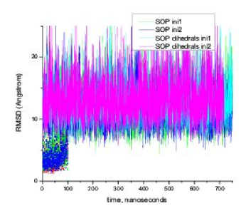
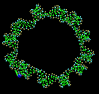
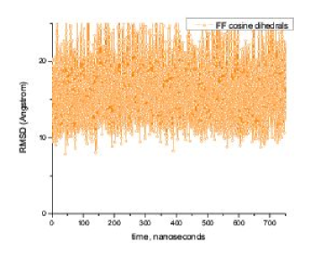
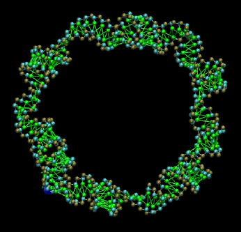
Figure 9: Left: RMSD for different variants of the parameter sets of the CG model in the equilibration CG runs. The data for the nanoring are plotted with lines and open circles (”FF cosine dihedrals”), while those for the dodecamer are plotted with small symbols (in the interval up to $100$ ns only). Right: The final snapshots of the RNA nanoring after $750$ ns equilibration in the CG model with the ”SOP dihedrals” (top) and ”FF cosine dihedrals” (bottom) parameter set.

Second, in the light of the RNA conformation classes, another important finding is that a simple modification of the dihedral function Eq. 7 allowed us to reach the SOP precision in describing the RNA nanoring by properly accommodating the distortions of the dihedrals in the kissing loops. Presently, the function Eq. 7 has only one additional dihedral minimum separated from the original one by $180^{\circ}$, i.e. only one additional conformation class (together with the main one for the A-form double helix). In principle, the dihedral function can be made more complex (e.g. to contain multiple minima). Note that the number of observed conformation classes is limited by at most ten Wadley et al. (2007). Therefore, one can hope to keep the dihedral functions (for both PSPS and SPSP dihedrals) reasonably simple yet fairly universal, which opens up a promising avenue towards a forcefield-like universal RNA CG model.

In this context it is interesting to establish a more detailed connection between the RNA conformation classes from Wadley et al. (2007) and the ones that we observe in our simulations. According to Wadley et al. (2007), a conformation class is defined by a pair of $(P_{i}S_{i}P_{i+1}S_{i+1})$ and $(S_{i-1}P_{i}S_{i}P_{i+1})$ dihedrals centered around a sugar $S_{i}$. Note that alternatively one can also select dihedral pairs centered around a phosphate $P_{i}$, i.e. $(S_{i-1}P_{i}S_{i}P_{i+1})$ and $(P_{i-1}S_{i-1}P_{i}S_{i})$. Using the RNA nanoring dihedrals from 6, we plotted 2D maps for both variants (10). The main double-helical peak at $(-153^{\circ},169^{\circ})$ is clearly visible, along with the two shoulders extending in the PSPS direction (cf. 5). In the terminology of Wadley et al. (2007) the shoulders correspond to the classes VI (cross-stem stacking of the purine-purine base pairs) and IV (absent stacking on the 3’ side of the nucleotide). The former is present in the nanoring because of a cross-stem stacking G-G pair just near the base of each loop Lee and Crothers (1998), the latter is probably found in the middle of the nanoring sides (we did not analyse this in detail).

Two more classes are found in the kissing loops (10, top). Namely, there are (i) 12 nucleotides (one per each kissing loop side) that have strongly deviating cis PSPS angles and double-helical trans SPSP angles, and (ii) immediately following them in the 5’ to 3’ sense, 12 other nucleotides that have the situation reversed, i.e. cis SPSP angles and trans PSPS angles. These nucleotides (found near sharp kinks of the nucleic backbone visible in 2) are the last ones base paired within their own chain and the first ones participating in the cross–chain base pairing in the kissing loops, respectively. While we can relate our class (ii) to the class II from Wadley et al. (2007), our class (i) seems to be absent from the scheme of Wadley et al. (2007). Interestingly, two classes (i) and (ii) collapse into a single one if the 2D dihedral map is replotted with the dihedral pairs centered around the phosphates (10, bottom). The reason for this is clear for the case of the nanoring, where the nucleotides of the classes (i) and (ii) are neighbours in the chain, but one may wonder whether a similar procedure applied to all the volume of data analysed in Wadley et al. (2007) would lead to a simplification of the observed conformation classes. Note, that the classification based on the phosphates (“suites”), and not on the nucleotides has already been used for the full RNA conformational space Murray et al. (2003).

Thus, we incorporated only the classes (i) and (ii) [collapsing to a single class if reformulated as specified above] into the FF–cosine–dihedrals variant of our CG model, and ignored the remaining two classes present in the nanoring [IV and VI according to Wadley et al. (2007)]. All these classes are obviously accounted for in the SOP–dihedrals variant. This explains slightly elevated values of RMSD in the former case, compared to the latter, though one extra class alone proved to be sufficient to model the kissing loops reasonably well.

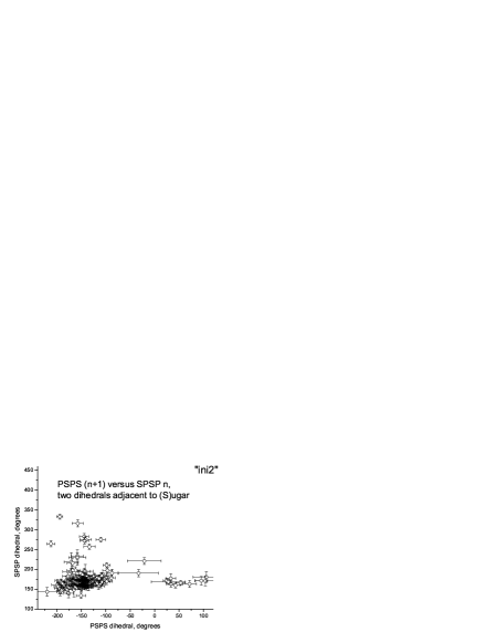
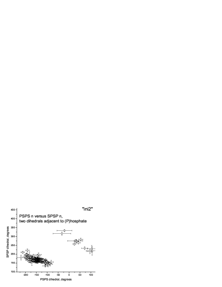
Figure 10: The 2D maps of the dihedral pair distributions of the RNA nanoring. Top: for the dihedral pairs centered around the sugars. Bottom: for the dihedral pairs centered around the phosphates.

VI Conclusions

In the present paper we reported a series of bead-based CG models for RNA with varying amounts of atomistic structural information and numbers of beads per nucleotide. They range from SOP ones, where all the specific values of bonds/angles/dihedrals from a reference structure (nanoring) are included in the model, to a forcefield approach, where the CG model is described by a few universal parameters. We started from the purely double-helical set of parameters derived from all-atom MD data for an RNA dodecamer, and applied it to the RNA nanoring, introducing the non-helical features whenever necessary. We are concluding here that the models with just one bead per nucleotide suffer from the effects of insufficient excluded volume, while the models with three beads per nucleotide [(P)hosphate, (S)ugar, (B)ase] are more suitable for the description of the RNA. The inclusion of just the detailed information about the (PSPS) and (SPSP) dihedral angles in the model renders precision similar to the inclusion of all available atomistic structural information, which illustrates the usefulness and robustness of the reduced (P-C4’) representation of the nucleic backbone Wadley et al. (2007). Furthermore, the existence of the quasi-discrete RNA conformation classes based on these dihedrals Wadley et al. (2007) is supported by our data too. For the simple non-helical conformation of the kissing loops we were able to design a dihedral potential function Eq. 7, that, while including only a single additional minimum, successfully accommodated local dihedral distortions. This opens up the road towards the development of even more transferable RNA CG models based on the P-C4’ conformation classes. 1 lists the values of the parameters ($26$ in total) for the 3B CG model we obtained. For the systems of thousands of nucleotides, a time scale of microseconds can be easily reached with the developed CG model. The structural precision of our 3B models in terms of RMSD is $\sim 0.06$ Å per nucleotide [to be compared e.g. with $\sim 0.1$ Å for another recent 3B model Ding et al. (2008) and $\sim 0.13$ Å for a 1B model Jonikas et al. (2009)].

Finally, we mention several directions for future development of our RNA CG model. Explicit electrostatics between phosphates as well as the sequence-specificity in the base-pair interactions will be incorporated. Besides, if the interaction between base pairs were treated in a non-bonding manner, this would allow one to study the association/dissociation reactions between the building blocks of the nanoring and other RNA nanostructures.

VII Supplemental information

The following extras can be of interest for some readers and is available on request: (i) details of the all-atom MD simulations used as sources for CG model fitting; (ii) details of the 1B CG model simulations; (iii) full set of graphs for all CG degrees of freedom.

3B CG model parameters
Backbone bonds
	$r_{0}$	$k$
$(P_{i}S_{i})$	3.93	133.4
$(S_{i}P_{i+1})$	3.92	107.8
$(S_{i}B_{i})$	3.38	61.3
Base pairing bonds
	$r_{0}$	$k$
$(B_{i}B_{j})$	8.99	16.5
$(B_{i+1}B_{j})$	6.86	2.83
$(B_{i+2}B_{j})$	7.35	2.93
Backbone angles
	$\theta_{0}$	$k$
$(P_{i}S_{i}P_{i+1})$	1.733 ($99.3^{\circ}$)	26.3
$(S_{i}P_{i+1}S_{i+1})$	1.819 ($104.2^{\circ}$)	106.9
$(P_{i}S_{i}B_{i})$	1.728 ($99.0^{\circ}$)	32.1
$(B_{i}S_{i}P_{i+1})$	1.642 ($94.1^{\circ}$)	127.2
Backbone dihedrals
	$\phi_{0}$	$k$
$(P_{i}S_{i}P_{i+1}S_{i+1})$	-2.677 ($-153.4^{\circ}$)	5.86
$(S_{i}P_{i+1}S_{i+1}P_{i+2})$	2.948 ($168.9^{\circ}$)	16.2
WCA potential for nonbonded pairs
	$\sigma$	$\varepsilon$
all	5.0	0.1
Excluded bonds (see the text)
$(S_{i}B_{i+1})$	$(B_{i}S_{i+1})$	$(B_{i}B_{i+1})$

Table 1: Parameters of 3B CG model. The distances are expressed in Å, the angles and dihedrals are expressed in radians (the values in degrees are shown for convenience too). The unit of energy is kcal/mol, and the units for the coefficients are derived from the unit of energy and Å or radians respectively. The nucleotide index $i$ is counted from the 5’ end.

References

- Jaeger and Chworos (2006) Jaeger, L.; Chworos, A. The architectonics of programmable RNA and DNA nanostructures. Current Opinion in Structural Biology 2006, 16, 531.
- Jaeger et al. (2001) Jaeger, L.; Westhof, E.; Leontis, N. TectoRNA: modular assembly units for the construction of RNA nano-objects. Nucleic Acids Research. 2001, 29, 455.
- Holbrook (2005) Holbrook, S. R. RNA structure: the long and the short of it. Current Opinion in Structural Biology 2005, 15, 302.
- Yingling and Shapiro (2007) Yingling, Y. G.; Shapiro, B. A. Computational design of an RNA hexagonal nano-ring and an RNA nanotube. Nano Letters 2007, 7, 2328.
- Sponer and Lankas (2006) Computational studies of RNA and DNA; Sponer, J., Lankas, F., Eds.; Springer, 2006; Vol. 2.
- Paliy et al. (2009) Paliy, M.; Melnik, R.; Shapiro, B. A. Molecular dynamics study of the RNA ring nanostructure: a phenomenon of self-stabilization. Physical Biology 2009, 6, 046003.
- Reith et al. (2003) Reith, D.; P tz, M.; M ller-Plathe, F. Deriving effective mesoscale potentials from atomistic simulations. Journal of Computational Chemistry 2003, 24, 1624–1636.
- Lyubartsev and Laaksonen (1995) Lyubartsev, A. P.; Laaksonen, A. Calculation of effective interaction potentials from radial distribution functions: A reverse Monte Carlo approach. Phys. Rev. E 1995, 52, 3730–.
- Ercolessi and Adams (1994) Ercolessi, F.; Adams, J. B. Interatomic Potentials From 1st-principles Calculations - the Force-matching Method. Europhysics Letters 1994, 26, 583–588.
- Voth (2009) Coarse-Graining of Condensed Phase and Biomolecular Systems; Voth, G. A., Ed.; CRC Press, 2009.
- Izvekov and Voth (2005) Izvekov, S.; Voth, G. A. A Multiscale Coarse-Graining Method for Biomolecular Systems. The Journal of Physical Chemistry B 2005, 109, 2469–.
- Noid et al. (2008) Noid, W. G.; Chu, J.-W.; Ayton, G. S.; Krishna, V.; Izvekov, S.; Voth, G. A.; Das, A.; Andersen, H. C. The multiscale coarse-graining method. I. A rigorous bridge between atomistic and coarse-grained models. J. Chem. Phys. 2008, 128, 244114–11.
- Noid et al. (2008) Noid, W. G.; Liu, P.; Wang, Y.; Chu, J.-W.; Ayton, G. S.; Izvekov, S.; Andersen, H. C.; Voth, G. A. The multiscale coarse-graining method. II. Numerical implementation for coarse-grained molecular models. J. Chem. Phys. 2008, 128, 244115–20.
- Tozzini (2005) Tozzini, V. Coarse-grained models for proteins. Current Opinion in Structural Biology 2005, 15, 144.
- Trovato and Tozzini (2008) Trovato, F.; Tozzini, V. Supercoiling and Local Denaturation of Plasmids with a Minimalist DNA Model. The Journal of Physical Chemistry B 2008, 112, 13197–.
- Ouldridge et al. (2009) Ouldridge, T. E.; Johnston, I. G.; Louis, A. A.; Doye, J. P. K. The self-assembly of DNA Holliday junctions studied with a minimal model. J. Chem. Phys. 2009, 130, 065101–11.
- Ghosh and Faller (2007) Ghosh, J.; Faller, R. State point dependence of systematically coarse-grained potentials. Molecular Simulation 2007, 33, 759–767.
- Nielsen et al. (2004) Nielsen, S. O.; Lopez, C. F.; Srinivas, G.; Klein, M. L. Coarse grain models and the computer simulation of soft materials. Journal of Physics: Condensed Matter 2004, 16, R481–R512.
- Hyeon and Thirumalai (2005) Hyeon, C.; Thirumalai, D. Mechanical unfolding of RNA hairpins. Proceedings of the National Academy of Sciences of the United States of America 2005, 102, 6789–6794.
- Hyeon and Thirumalai (2007) Hyeon, C.; Thirumalai, D. Mechanical Unfolding of RNA: From Hairpins to Structures with Internal Multiloops. Biophysical Journal 2007, 92, 731.
- Hyeon et al. (2006) Hyeon, C.; Dima, R.; Thirumalai, D. Pathways and Kinetic Barriers in Mechanical Unforlding and Refolding of RNA and Proteins. Structure 2006, 14, 1644.
- Trylska et al. (2005) Trylska, J.; Tozzini, V.; McCammon, J. A. Exploring Global Motions and Correlations in the Ribosome. Biophysical Journal 2005, 89, 1455 – 1463.
- Jonikas et al. (2009) Jonikas, M. A.; Radmer, R. J.; Laederach, A.; Das, R.; Pearlman, S.; Herschlag, D.; Altman, R. B. Coarse-grained modeling of large RNA molecules with knowledge-based potentials and structural filters. Rna-a Publication of the Rna Society 2009, 15, 189–199.
- Pincus et al. (2008) Pincus, D. L.; Cho, S. S.; Hyeon, C.; Thirumalai, D. Chapter 6 Minimal Models for Proteins and RNA: From Folding to Function. In Molecular Biology of Protein Folding, Part B; Conn, P. M., Ed.; Academic Press, 2008; Vol. Volume 84, pp 203–250.
- Ding et al. (2008) Ding, F.; Sharma, S.; Chalasani, P.; Demidov, V. V.; Broude, N. E.; Dokholyan, N. V. Ab initio RNA folding by discrete molecular dynamics: From structure prediction to folding mechanisms. RNA 2008, 14, 1164–1173.
- Gherghe et al. (2009) Gherghe, C. M.; Leonard, C. W.; Ding, F.; Dokholyan, N. V.; Weeks, K. M. Native-like RNA Tertiary Structures Using a Sequence-Encoded Cleavage Agent and Refinement by Discrete Molecular Dynamics. Journal of the American Chemical Society 2009, 131, 2541–2546.
- CAO and CHEN (2005) CAO, S.; CHEN, S.-J. Predicting RNA folding thermodynamics with a reduced chain representation model. RNA 2005, 11, 1884–1897.
- Cao and Chen (2009) Cao, S.; Chen, S.-J. Predicting structures and stabilities for H-type pseudoknots with interhelix loops. RNA 2009, 15, 696–706.
- Das and Baker (2007) Das, R.; Baker, D. Automated de novo prediction of native-like RNA tertiary structures. Proceedings of the National Academy of Sciences 2007, 104, 14664–14669.
- Parisien and Major (2008) Parisien, M.; Major, F. The MC-Fold and MC-Sym pipeline infers RNA structure from sequence data. Nature 2008, 452, 51–55.
- Tan et al. (2006) Tan, R. K. Z.; Petrov, A. S.; Harvey, S. C. YUP: A Molecular Simulation Program for Coarse-Grained and Multiscaled Models. Journal of Chemical Theory and Computation 2006, 2, 529–540.
- Shapiro et al. (2007) Shapiro, B. A.; Yingling, Y. G.; Kasprzak, W.; Bindewald, E. Bridging the gap in RNA structure prediction. Current Opinion in Structural Biology 2007, 17, 157–165.
- Knotts et al. (2007) Knotts, T. A.; IV,; Rathore, N.; Schwartz, D. C.; de Pablo, J. J. A coarse grain model for DNA. J. Chem. Phys. 2007, 126, 084901–12.
- Sambriski et al. (2009) Sambriski, E.; Schwartz, D.; de Pablo, J. A Mesoscale Model of DNA and Its Renaturation. Biophysical Journal 2009, 96, 1675–1690.
- Wadley et al. (2007) Wadley, L. M.; Keating, K. S.; Duarte, C. M.; Pyle, A. M. Evaluating and Learning from RNA Pseudotorsional Space: Quantitative Validation of a Reduced Representation for RNA Structure. Journal of Molecular Biology 2007, 372, 942 – 957.
- Lee and Crothers (1998) Lee, A. J.; Crothers, D. M. The solution structure of an RNA loop-loop complex: the ColE1 inverted loop sequence. Structure 1998, 6, 993–1005.
- Weeks et al. (1971) Weeks, J. D.; Chandler, D.; Andersen, H. C. Role of Repulsive Forces in Determining the Equilibrium Structure of Simple Liquids. J. Chem. Phys. 1971, 54, 5237–5247.
- Smith et al. (2002) Smith, W.; Yong, C. W.; Rodger, P. M. DL_POLY: application to molecular simulation. Molecular Simulation 2002, 28, 385–471.
- Evans and Morris (1984) Evans, D. J.; Morris, G. P. Non-Newtonian molecular dynamics. Computer Phys. Reports 1984, 1, 297–343.
- Humphrey et al. (1996) Humphrey, W.; Dalke, A.; Schulten, K. VMD – Visual Molecular Dynamics. Journal of Molecular Graphics 1996, 14, 33–38.
- Murray et al. (2003) Murray, L. J. W.; Arendall, W. B.; Richardson, D. C.; Richardson, J. S. RNA backbone is rotameric. Proceedings of the National Academy of Sciences of the United States of America 2003, 100, 13904–13909.