Circumstellar molecular composition of the oxygen-rich AGB star IK Tau: I. Observations and LTE chemical abundance analysis

Abstract

Context. Molecular lines in the (sub)millimeter wavelength range can provide important information about the physical and chemical conditions in the circumstellar envelopes around Asymptotic Giant Branch stars.

Aims. The aim of this paper is to study the molecular composition in the circumstellar envelope around the oxygen-rich star IK~Tau.

Methods. We observed IK Tau in several (sub)millimeter bands using the APEX telescope during three observing periods. To determine the spatial distribution of the $\mathrm{{}^{12}CO(3-2)}$ emission, mapping observations were performed. To constrain the physical conditions in the circumstellar envelope, multiple rotational CO emission lines were modeled using a non local thermodynamic equilibrium radiative transfer code. The rotational temperatures and the abundances of the other molecules were obtained assuming local thermodynamic equilibrium.

Results. An oxygen-rich Asymptotic Giant Branch star has been surveyed in the submillimeter wavelength range. Thirty four transitions of twelve molecular species, including maser lines, were detected. The kinetic temperature of the envelope was determined and the molecular abundance fractions of the molecules were estimated. The deduced molecular abundances were compared with observations and modeling from the literature and agree within a factor of 10, except for SO₂, which is found to be almost a factor 100 stronger than predicted by chemical models.

Conclusions. From this study, we found that IK Tau is a good laboratory to study the conditions in circumstellar envelopes around oxygen-rich stars with (sub)millimeter-wavelength molecular lines. We could also expect from this study that the molecules in the circumstellar envelope can be explained more faithful by non-LTE analysis with lower and higher transition lines than by simple LTE analysis with only lower transition lines. In particular, the observed CO line profiles could be well reproduced by a simple expanding envelope model with a power law structure.

1 Introduction

Stars with initial masses lower than $\sim$8 $\mathrm{M_{\odot}}$ evolve to a pulsationally unstable red giant star on the Asymptotic Giant Branch (AGB). At this stage, mass loss from the evolved central star produces an expanding envelope. Further on, carbon, C, is fused in the core and then oxygen, O (Yamamura et al. 1996; Fukasaku et al. 1994).

AGB stars are characterized by low surface temperatures, $T_{*}\mathrm{\leq 3000}$ K, high luminosities up to several $\mathrm{10^{4}}$ $\mathrm{L_{\odot}}$, and a very large geometrical size up to several AU (Habing 1996). In general, these highly evolved stars are surrounded by envelopes with expansion velocities between 5 $\mathrm{km\,s^{-1}}$ and 40 $\mathrm{km\,s^{-1}}$. They have high mass-loss rates between $\mathrm{10^{-8}}$ and $\mathrm{10^{-4}\,M_{\odot}\,yr^{-1}}$. Their atmospheres provide favorable thermodynamic conditions for the formation of simple molecules, due to the low temperatures and, simultaneously, high densities. Due to pulsation, molecules may reach a distance at which the temperature is lower than the condensation temperature and at which the density is still high enough for dust grains to form. Radiation pressure drives the dust away from the star. Molecules surviving dust formation are accelerated due to dust-grain collisions (Goldreich & Scoville 1976).

The chemistry of the atmospheres and, further out, of the circumstellar envelopes (CSEs) around AGB stars is dependent on the chemical class. They are classified either as M stars (C/O abundance ratio $<$ 1), S stars (C/O $\approx$ 1) or C stars (C/O $>$ 1). The optical and infrared spectra of AGB stars show absorption from the stellar atmosphere. M-type stellar spectra are dominated by lines of oxygen-bearing molecules, e.g., the metal oxides SiO and TiO, and $\mathrm{H_{2}O}$. In C-star atmospheres carbon-bearing molecules like, a.o., CH, C₂, $\mathrm{C_{2}H_{2}}$ and HCN are detected at optical and infrared wavelenths, and in the microwave regime (e.g. Gautschy-Loidl et al. 2004). While the atmospheric abundance fractions are nowadays quite well understood in terms of initial chemical composition, which may be altered by nucleosynthetic products which are brought to the surface due to dredge-ups, the main processes determining the circumstellar chemical abundance stratification of many molecules are still largely not understood. In the stellar photosphere, the high gas density ensures thermal equilibrium (TE). Pulsation-driven shocks in the inner wind region suppress TE. This region of strong shock activity is also the locus of grain formation, resulting in the depletion of few molecules as SiO and SiS. Other molecules, as CO and CS, are thought to be inreactive in the dust forming region (Duari et al. 1999). At larger radii, the so-called outer envelope is penetrated by ultraviolet interstellar photons and cosmic rays resulting in a chemistry governed by photochemical and ion-molecule reactions. This picture on the chemical processes altering the abundance stratification is generally accepted, but many details on chemical reactions rates, molecular left-overs after the dust formation, shock strengths inducing a fast chemistry zone etc. are not yet known.

Spectroscopical studies of molecular lines in the (sub)millimeter range are a very useful tool for estimating the physical and chemical conditions in CSEs. Due to its proximity, the carbon-rich AGB star IRC+10216 has attracted lot of attention, resulting in the detection of more than 60 different chemical compounds in its CSE (e.g. Ridgway et al. 1976; Cernicharo et al. 2000). Until now, detailed studies of oxygen-rich envelopes have been rare. Recently, Ziurys et al. (2004) have focused on the chemical analysis of the oxygen-rich peculiar red supergiant VY~CMa. VY CMa is, however, not a proto-type of an evolved oxygen-rich star. A complex geometry is deduced from Hubble Space Telescope images (Smith et al. 2001) with a luminosity larger than $\,10^{5}$ L_⊙ and a mass-loss rate of $\sim$$2\times 10^{-4}$ M_⊙/yr (Bowers et al. 1983; Sopka et al. 1985). VY CMa is a spectacular object, which because of its extreme evolutionary state can explode as a supernova at any time. Interpreting the molecular emission profiles of VY CMa is therefore a very complex task, subject to many uncertainties. To enlarge our insight in the chemical structure in the envelopes of oxygen-rich low and intermediate mass stars, we therefore have started a submillimeter survey on the oxygen-rich AGB star IK~Tau, which is thought to be (roughly) spherically symmetric (Lane et al. 1987; Marvel 2005). We thereby will advance the understanding on the final stages of stellar evolution of the majority of stars in galaxies as our Milky Way and their resultant impact on the interstellar medium and the cosmic cycle.

1.1 IK Tau

The Mira variable IK Tau, also known as NML Tau, is located at $\alpha_{2000}$=$3^{\mathrm{h}}53^{\mathrm{m}}28^{\mathrm{s}}$.8, $\delta_{2000}$=$11^{\circ}24^{\prime}23^{\prime\prime}$. It was found to be an extremely cool star having large infrared ($J-K$) excess (Alcolea et al. 1999) consistent with a 2000 K blackbody. IK Tau shows regular optical variations with an amplitude of $\sim$ 4.5 mag.

IK Tau is an O-rich star of spectral type ranging from M8.1 to M11.2 (Wing & Lockwood 1973). Its distance was derived by Olofsson et al. (1998) to be 250 pc assuming a stellar temperature of 2000 K. The pulsation period is $\sim$470 days (Hale et al. 1997). The systemic velocity of the star is 33.7 $\mathrm{km\,s^{-1}}$. Mass-loss rate estimates range from $\mathrm{2.4\times 10^{-6}}$ $\mathrm{M_{\odot}\,yr^{-1}}$ (from the CO(J=1-0) line; Olofsson et al. 1998) to $\mathrm{3\times 10^{-5}}$ $\mathrm{M_{\odot}\,yr^{-1}}$ (from an analysis of multiple SiO lines; González Delgado et al. 2003).

In the circumstellar envelope of IK Tau maser emission from OH (Bowers et al. 1989), $\mathrm{H_{2}O}$ (Lane et al. 1987), and SiO (Boboltz & Diamond 2005) and thermal emission of SiO, CO, SiS, SO, $\mathrm{SO_{2}}$ and HCN have previously been found (Lindqvist et al. 1988; Bujarrabal et al. 1994; Omont et al. 1993). Obviously, IK Tau is a prime candidate for circumstellar chemistry studies.

2 Observations

Table 1: Overview of the molecular line transitions observed with APEX.

Species	Transition	$\nu$ (MHz)	HPBW (″)
12CO	3 - 2	345796.00	18
	4 - 3	461040.78	14
	7 - 6	806651.81	8
13CO	33 - 22	330587.94	19
SiS	16 - 15	290380.31	21
	17 - 16	308515.63	20
	19 - 18	344778.78	18
	20 - 19	362906.34	18
28SiO	7 - 6	303926.81	20
	8 - 7	347330.59	18
29SiO	7 - 6	300120.47	20
	8 - 7	342980.84	18
30SiO	7 - 6	296575.75	21
	8 - 7	338930.03	18
SO	77 - 66	301286.13	20
	88 - 77	344310.63	18
SO2	33 1 - 22 0	313279.72	20
	171 17 - 160 16	313660.84	20
	43 1 - 32 2	332505.25	19
	132 12 -121 11	345338.53	18
	53 3 - 42 2	351257.22	18
	144 10 - 143 11	351873.88	18
CS	6 - 5	293912.25	21
	7 - 6	342883.00	18
HCN	4 - 3	354505.47	18
CN	N=3 - 2, J=5/2 -3/2	340031.56	18
	N=3 - 2, J=7/2 -5/2	340247.78	18
masers
H2O	102 9 - 93 6	321225.63	19
	51 5 - 42 2	325152.91	19
28SiO	v=1, 7 - 6	301814.30	20
	v=1, 8 - 7	344916.35	18
	v=3, 7 - 6	297595.41	20
29SiO	v=1, 7 - 6	298047.33	20
30SiO	v=1, 8 - 7	336602.44	19

The observations were performed with the APEX 12 m telescope in Chile (Güsten et al. 2006) located at the 5100 m high site on Llano de Chajnantor. The data were obtained during observing periods in 2005 November, 2006 April and August. The receivers used were the facility APEX-2A (Risacher et al. 2006) and the MPIfR FLASH receivers (Heyminck et al. 2006). Typical system noise temperatures were about 200 K – 1000 K at 290 GHz and 350 GHz, 1000 K at 460 GHz and 5000 K at 810 GHz, respectively. The spectrometers for the observations were Fast Fourier Transform Spectrometers (FFTS) with 1 GHz bandwidth and the channel width for the 290–350 GHz observations was approximately 122.07 kHz (8192 channels), and for the 460 GHz and 810 GHz observations 488.28 kHz (2048 channels). For the observations, a position-switching mode was used with the reference position typically 180^′′ off-source. The antenna was focused on the available planets. IK Tau itself was strong enough to serve as a line pointing source, thus small cross scans in the ¹²CO(3-2) line were done to monitor the pointing during the observations. The telescope beam sizes (HPBW) at frequencies of the observed molecular lines are shown in Table 1. The antenna beam efficiencies are given in Table 2 of Güsten et al. (2006).

To map the circumstellar envelope in the ¹²CO(3-2) line, 30 positions distributed on a 5$\times$6 grid in right ascension and declination were observed. The grid spacing was 9^′′ (half the FWHM beam size at 345 GHz). A raster mapping procedure was used along the parallel grid lines with an integration time of 15 s.

Table 2: Beam efficiencies for the different receivers.

Receiver	Forward efficiency	Beam efficiency
APEX-2A 290 GHz	0.97	0.80
APEX-2A 350 GHz	0.97	0.73
FLASH 460 GHz	0.95	0.60
FLASH 810 GHz	0.95	0.43

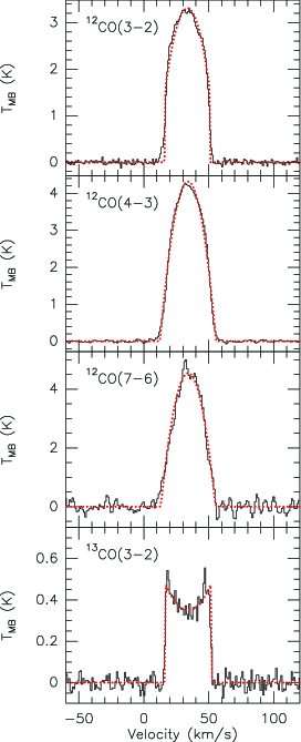
Figure 1: Observed $\mathrm{{}^{12}CO}$ and $\mathrm{{}^{13}CO}$ line profiles (solid lines) together with the expanding shell fit (dotted lines).

The spectra were reduced using the CLASS program of the IRAM GILDAS. To calculate the main-beam brightness temperatures of the lines, $T_{\mathrm{MB}}$, the following relation was used:

$$T_{\mathrm{MB}}={T_{\mathrm{A}}^{*}}\frac{\eta_{\mathrm{f}}}{\eta_{\mathrm{eff}}}\,.$$ (1)

Here $T_{\mathrm{A}}^{*}$ is the measured antenna temperature, $\eta_{\mathrm{{f}}}$ is the forward efficiency and $\eta_{\mathrm{{eff}}}$ is the antenna main-beam efficiency of APEX (see Table 2).

3 Observational results

Thirty four transitions from 12 molecular species including maser lines were detected with the APEX telescope toward IK Tau. The detected molecular lines are listed in Table 1 and their spectra are displayed in Figs. 1 to 5.

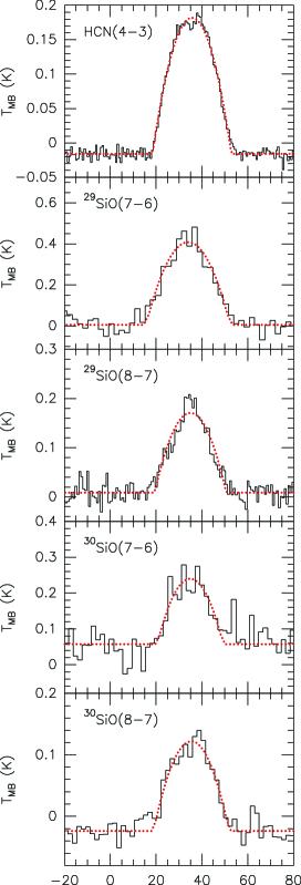
Figure 2: Observed HCN, $\mathrm{{}^{29}SiO}$ and $\mathrm{{}^{30}SiO}$ line profiles (solid lines) together with the expanding shell fit (dotted lines).

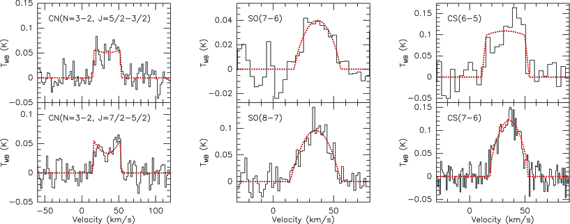
Figure 3: Observed CN, SO and CS line profiles (solid lines) together with the expanding shell fit (dotted lines).

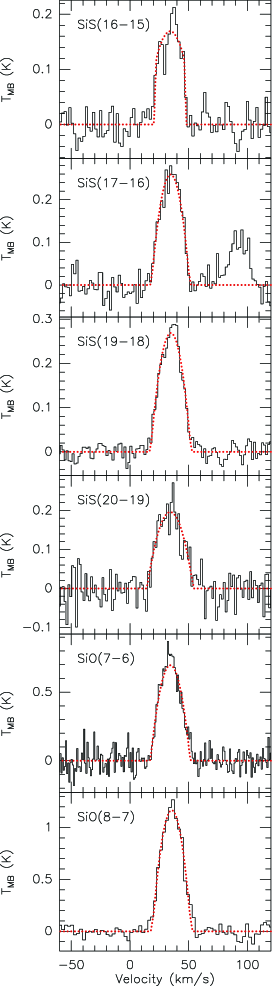
Figure 4: Observed SiS and SiO line profiles (solid lines) together with the expanding shell fit (dotted lines).

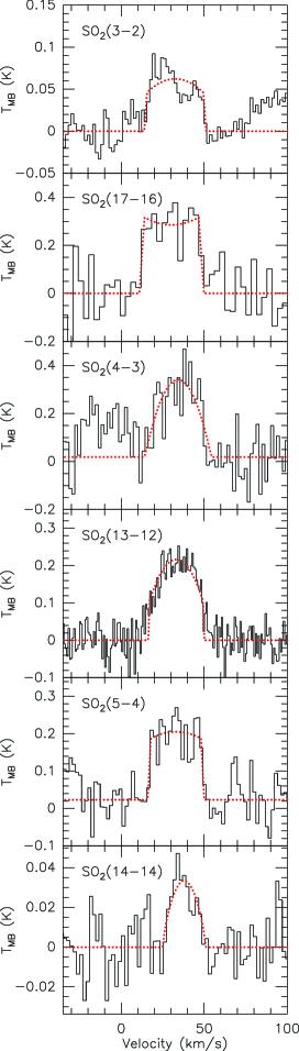
Figure 5: Observed $\mathrm{SO_{2}}$ line profiles (solid lines) together with the expanding shell fit (dotted lines).

Fig. 6 and Fig. 7 show the $\mathrm{H_{2}O}$ maser lines and SiO maser lines observed toward IK Tau, respectively; the maser line parameters are given in Table 3. Maser emission from $\mathrm{H_{2}O}$ at 321 GHz and 325 GHz was detected, as well as in the $J=7-6$ and $J=8-7$ rotational transitions within the $v=1$ and $v=3$ vibrationally excited states of $\mathrm{{}^{28}SiO}$, $\mathrm{{}^{29}SiO}$ and $\mathrm{{}^{30}SiO}$.

Figure 6: 321 GHz and 325 GHz $\mathrm{H_{2}O}$ maser emissions observed towards IK Tau.

Figure 7: $\mathrm{{}^{28}SiO}$, $\mathrm{{}^{29}SiO}$ and $\mathrm{{}^{30}SiO}$ maser emission detected in the rotational transitions $J=7-6$ and $J=8-7$ of the fundamental $v$=1 and $v$=3 vibrational excited states observed towards IK Tau.

3.1 Line parameters

Table 3: Line parameters for the detected maser lines.

		$\mathrm{T_{MB}}$ peak (K)	Profile $\mathrm{T_{MB}}$ area (K   km s-1)
Species	Transition	Bright temp. estimate	Bright temp. estimate	$\mathrm{V_{lsr}}$ (km s-1)
H2O	102 9 - 93 6	1.36	4.31	33.4
	51 5 - 42 2	2.09	37.9	35.0
28SiO	V=1, 7 - 6	0.44	3.64	32.5
	V=1, 8 - 7	0.29	1.00	34.6
	V=3, 7 - 6	0.36	1.22	33.4
29SiO	V=1, 7 - 6	0.41	1.63	32.9
30SiO	V=1, 8 - 7	1.40	5.4	33.8

Table 4: Line parameters for each (non-masering) transition.

				$\mathrm{T_{MB}}$ peak (K) /	Profile $\mathrm{T_{MB}}$ area (K   km s-1) /
Species	Transition	$\frac{\mathrm{Eu}}{\mathrm{k}}$ (K)	$\mu_{0}^{2}$S (Debye2)	Mean $\mathrm{T_{b}}$	Integrated mean $\mathrm{T_{b}}$	Vexp (km s-1)
12CO	3 - 2	33.2	0.04	3.31 / 5.99	95.7 / 173	17.3
	4 - 3	55.3	0.05	4.25 / 6.33	125 / 186	21.2
	7 - 6	155	0.08	5.04 / 5.85	129 / 149	21.0
13CO	3 - 2	31.7	0.04	0.58 / 1.10	15.2 / 23.0	17.8
SiS	16 - 15	118	47.9	0.21 / 19.3	3.91 / 360	12.9
	17 - 16	133	50.9	0.28 / 23.4	5.77 / 483	16.4
	19 - 18	166	56.9	0.29 / 19.7	6.33 / 430	17.3
	20 - 19	183	59.9	0.27 / 18.3	5.2 / 353	19.4
SiO	7 - 6	58.4	67.4	0.87 / 72.8	16.4 / 1373	17.0
	8 - 7	75.0	77.0	1.27 / 86.3	26.7 / 1813	16.5
SO	77 - 66	71.0	16.5	0.06 / 5.0	1.09 / 91.2	17.7
	88 - 77	87.5	18.9	0.27 / 18.3	4.72 / 321	21.0
SO2	33 1 - 22 0	27.6	6.64	0.09 / 7.5	2.16 / 181	17.8
	171 17 - 160 16	136	36.5	0.38 / 31.8	11.3 / 945	17.9
	43 1 - 32 2	31.3	6.92	0.07 / 5.3	1.41 / 107	19.4
	132 12 -121 11	93.0	13.4	0.25 / 17.0	6.34 / 43	16.5
	53 3 - 42 2	35.9	7.32	0.06 / 4.08	1.36 / 92.4	16.1
	144 10 - 143 11	136	19.6	0.05 / 3.40	0.55 / 37.4	12.1
CS	6 - 5	49.4	23.1	0.16 / 14.7	4.12 / 380	19.1
	7 - 6	65.8	27.0	0.15 / 10.2	3.07 / 209	16.6
29SiO	7 - 6	57.6	67.2	0.22 / 18.4	5.08 / 425	18.7
	8 - 7	74.1	76.8	0.27 / 18.3	4.72 / 321	15.1
30SiO	7 - 6	56.9	67.2	0.13 / 12.0	2.06 / 190	14.1
	8 - 7	73.2	76.8	0.15 / 10.2	2.88 / 196	16.4
HCN	4 - 3	42.5	108	0.69 / 15.8	15.3 / 249	17.0
CN	N=3 - 2, J=5/2 -3/2	32.6	6.72	0.08 / 5.44	1.98 / 135	18.5
	N=3 - 2, J=7/2 -5/2	32.7	9.01	0.07 / 4.76	1.60 / 109	18.7

To get the mean brightness temperature estimates, the spectra were corrected by the beam-filling factors assuming a CO source size of 17^′′ (Bujarrabal & Alcolea 1991), a HCN source size of 3.85^′′ (Marvel 2005) and source sizes for the other molecules of 2.2^′′ (Lucas et al. 1992). Note that the CO size may be uncertain, likely underestimated, since the signal-to-noise (S/N) ratios of the profiles obtained by Bujarrabal & Alcolea (1991) are much smaller than those of the CO profiles presented in this paper.

The beam-filling factor is given by

$$f=\frac{\theta_{\mathrm{S}}^{2}}{\theta_{\mathrm{S}}^{2}+\theta_{\mathrm{b}}^{2}}\,,$$ (2)

where $\theta_{\mathrm{S}}$ is the source size and $\theta_{\mathrm{b}}$ is the half-power beam width (HPBW) shown in Table 1. Both source and beam are assumed to be circular Gaussians. The mean brightness temperature estimate is computed by

$$T_{\mathrm{b}}=\frac{1}{f}T_{\mathrm{MB}}\,.$$ (3)

Line parameters were derived with CLASS (see more details on http://www.iram.fr/IRAMFR/GILDAS) from fitting the spectral lines with expanding shell fits, from which the expansion velocity of the envelope is obtained. The observed maser line and thermal emission line parameters are given in Table 3 and 4, including the envelope expansion velocity $V_{\mathrm{exp}}$, the main beam brightness temperature $T_{\mathrm{MB}}$, the integrated area, and the parameters of the expanding shell fits. The expansion velocities are distributed from 14 $\mathrm{km\,s^{-1}}$ to 21 $\mathrm{km\,s^{-1}}$.

When the S/N ratio is high enough to warrant a consideration of the shape of the line profiles, they appear to be characteristic for circumstellar envelopes (for more detail see Zuckerman 1987) : the $\mathrm{{}^{12}CO}$ lines have the parabolic shape of optically thick lines and the $\mathrm{{}^{13}CO}$($3-2$) line has the double-horn shape of spatially resolved optically thin lines (see Fig. 1). Lines from the three SiO isotopologues and SiS lines have a Gaussian shape (see Fig. 4), indicating that they are partially formed in the wind acceleration regime where the stellar winds has not yet reached its full terminal velocity (Bujarrabal & Alcolea 1991). Some of the $\mathrm{SO_{2}}$ lines seem to show the square shape characteristic of unresolved optically thin lines and some of them have the parabolic shape of optically thick lines (see Fig. 5). CS and SO lines seem to have the square shape of unresolved optically thin lines for low excitation transitions and the parabolic shape of optically thick lines for high excitation transitions (see Fig. 3). HCN shows a global parabolic shape with a weak double-peak profile on the top (see Fig. 2). For the CN molecule fits to the spectra were done that take the hyperfine structure of the molecule into account. Although the S/N of the individual components is small, the observations are not in agreement with the optical thin ratio of different HFS components and hint to hyperfine anomalies as already reported by Bachiller et al. (1997).

3.2 $\mathrm{CO}$ Maps

The spectra resulting from mapping the $\mathrm{{}^{12}CO(3-2)}$ transition in a region of 45^′′$\times$54^′′ around IK Tau are shown in Fig.  8. These spectra provide us with a tool to derive the source size as a function of radial velocity (see Fig. 9).The envelope of IK Tau appears roughly spherically symmetric in $\mathrm{{}^{12}CO(3-2)}$ with a deconvolved extent at half-peak integrated intensity of 20^′′. The physical diameter of the emission region is thus $2.1\times 10^{16}$ cm assuming a source distance of 250 pc.

Figure 8: Map of $\mathrm{{}^{12}CO}$ J=3-2 line emission toward IK Tau. The grid spacing was 9^′′. The main-beam brightness temperatures in the spectra range from 0.5 K to 3.3 K.

Figure 9: Contour maps of the $\mathrm{{}^{12}CO}$ J=3-2 line emission for IK Tau integrated over 10 $\mathrm{km\,s^{-1}}$ centered at velocities of 15 $\mathrm{km\,s^{-1}}$, 25 $\mathrm{km\,s^{-1}}$, 35 $\mathrm{km\,s^{-1}}$ and 45 $\mathrm{km\,s^{-1}}$. One velocity interval is centered near the stellar radial velocity of 33.7 $\mathrm{km\,s^{-1}}$.The contour values are 20 $\%$ to 90 $\%$ and 99 $\%$ of the maximum integrated intensity in each velocity interval, which is 7, 29, 32, and 26 $\mathrm{K\,km\,s^{-1}}$ for the 15, 25, 35, and 45 $\mathrm{km\,s^{-1}}$ channel, respectively. The 50 $\%$ contour level is drawn in boldface.

4 Modeling results

4.1 Physical structure of the envelope

CO lines are amongst the best tools to estimate the global properties of circumstellar envelopes, since the abundance of CO is quite constant across the envelope, except for photo-dissociation effects at the outer edge (Mamon et al. 1988). The spatial distribution of CO was found from our mapping observation to be spherically symmetric (see Sect. 3.2). A detailed multi-line non-LTE (non local thermodynamic equilibrium) study of CO can therefore be used to determine the physical properties of the envelope.

The one-dimensional version of the Monte Carlo code RATRAN (Hogerheijde & van der Tak 2000) was used to simulate the CO lines’ emission. The basic idea of the Monte Carlo method is to split the emergent radiative energies into photon packages, which perform a random walk through the model volume. This allows the separation of local and external contributions of the radiation field and makes it possible to calculate the radiative transfer and excitation of molecular lines. The Monte Carlo method for molecular line transfer has been described by Bernes (1979) for a spherically symmetric cloud with a uniform density. The code is formulated from the viewpoint of cells rather than photons. It shows accurate and fast performance even for high opacities (for more details see Hogerheijde & van der Tak 2000). The circumstellar envelope is assumed to be spherically symmetric, to be produced by a constant mass-loss rate, and to expand at a constant velocity. In the Monte Carlo simulation, typically $10^{3}$ model photons are followed throughout the envelope until they escape. The region is divided into discrete grid shells, each with constant properties (density, temperature, molecular abundance, turbulent line width, etc.).

For the case of a steady state, spherically symmetric outflow, the gas density as a function of radial distance from the center of the AGB star is given by

$$n(r)=\frac{\dot{M}}{4\pi r^{2}V_{\mathrm{exp}}m}\,,$$ (4)

where $m$ is the mass of the typical gas particle, taken to be $m\sim 3\times 10^{-24}$ gram, since the gas is mainly in molecular form in AGB envelopes (Teyssier et al. 2006).

The kinetic temperature is assumed to vary as

$$T=T_{0}\left[\frac{10^{16}}{r(\mathrm{cm})}\right]^{\alpha}+T_{\mathrm{bg}}\,,$$ (5)

where $T_{0}$ is the temperature at $1\times 10^{16}$ cm and $T_{\mathrm{bg}}$ represents the background temperature. With the radial profiles for density and temperature given by Eq. 4 and 5, the program solves for the molecular excitation as a function of radius. Beside collisional excitation, radiation from the cosmic microwave background and thermal radiation from local dust were taken into account. Then, the molecular emission is integrated in radial direction over the line of sight and convolved with the appropriate antenna beam.

The best-fit model is found by minimizing the total $\chi^{2}$ using the $\chi^{2}$ statistic defined as

$$\chi^{2}=\sum_{i=1}^{N}{\frac{[I_{\mathrm{mod}}-I_{\mathrm{obs}}]^{2}}{\sigma^{2}}}.$$ (6)

where $I_{\mathrm{mod}}$ is the line intensity of the model and $I_{\mathrm{obs}}$ is the observation, $\sigma$ is $rms$ noise of the observed spectra, the summation is done over all channels $N$ of the three ¹²CO line transitions as observed for this project with APEX, i.e. $J=3-2$, $J=4-3$, and $J=7-6$. We have put more weight on the reproduction of the line shapes and the fitting of the lines observed with the APEX telescope which were calibrated in a consistent way than on the reproduction of the lines taken from the literature. The reduced $\chi^{2}$ for the models is given by

$$\chi^{2}_{\mathrm{red}}=\frac{\chi^{2}}{d.f},$$ (7)

where $d.f$ is the degree of freedom being $N-p$, with $p$ the number of adjustable parameters. Fig. 10 shows the $\chi^{2}$ contour plot produced by varying the mass-loss rate and the temperature $T_{0}$. In this figure, the 68 % confidence limit, i.e. the 1$\sigma$ level, is indicated. In this region, the temperature $T_{0}$ ranges between 34 to 47 K and the mass-loss rate is in the range from 4.0$\times$10^-6 to 5.7$\times$10^-6 M_⊙/yr.

The best-fit model parameters are listed in Table 5; the results of the model fits are shown in Fig. 11. In Fig. 12 theoretical model predictions for the $\mathrm{{}^{12}CO}$ lines with different inner radii, different $T_{0}$, and different outer radii are shown. Predictions for $\mathrm{{}^{13}CO}$ with different $T_{0}$ are presented in Fig. 13. Predictions for intensities at the observed offset positions were done from the best fit model and are consistent with the size determined from the observed CO maps.

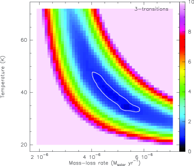
Figure 10: Reduced $\chi^{2}$ contour maps of the model to input variable parameters, i.e., the mass-loss rate ($\dot{M}$) and temperature ($T_{0}$), which is the kinetic temperature at a given radius ($1\times 10^{16}$ cm). The contour level is drawn at 0.94 indicating the 68 $\%$ confidence level.

As shown in Fig. 11, the overall line profiles are fit very well for the higher $J$ transitions ($\mathrm{{}^{12}CO(3-2)}$, $\mathrm{{}^{12}CO(4-3)}$, $\mathrm{{}^{12}CO(7-6)}$). However, the model intensities of the IRAM $\mathrm{{}^{12}CO(1-0)}$ and $\mathrm{{}^{12}CO(2-1)}$ transitions are somewhat higher than the observational data taken from literature, but the shapes fit satisfactorily. The predictions for the $\mathrm{{}^{12}CO(2-1)}$ line are still within the absolute uncertainty of the line, but this is not the case for the $\mathrm{{}^{12}CO(1-0)}$ line. An obvious reason for this mismatch could be a problem with the outer radius value. However, our sensitivity analysis (see Fig. 12 and see discussion in next paragraphs) shows that, while lowering the outer radius value indeed the total integrated intensity decreases, the line shape is not well reproduced anymore. Since the relative uncertainty (i.e., the line shape) is much lower than the absolute intensity (i.e., the integrated intensity), we have put more weight on the reproduction of the line shapes. Moreover, we note that this is not the first time that a non-compatability of the IRAM fluxes with other observed data is reported (e.g. Decin et al. 2008). The $\mathrm{{}^{13}CO(3-2)}$ line clearly shows a double-horn profile and the best-fit results in a somewhat different $T_{0}$ and a different outer radius than for the ¹²CO data. Nevertheless, the best-fit value for $T_{0}$ derived from $\mathrm{{}^{12}CO}$ still gives a reasonable fit to the $\mathrm{{}^{13}CO}$ line (Fig. 13). As shown in Fig. 13, the intensities of the profiles do not change so much with $T_{0}$ but the lines show a flat shape on top for the lower temperatures (30 K and 40 K), and a double-horn shape at higher temperatures.

As shown in Fig. 12, the line shapes and intensities for all transitions are not much influenced by the inner radius variations since the $\mathrm{{}^{12}CO}$ emission contributing dominantly to the spectra arises from regions further out in the envelope. The outer radius variations mainly affect the $\mathrm{{}^{12}CO(1-0)}$ line, which is formed further out in the envelope than the other $\mathrm{{}^{12}CO}$ transitions.

Table 5: Parameters for the best-fit model to the observed ¹²CO and ¹³CO line profiles.

	Ri	Rout	Mass-loss late	fCO	Vexp	T0	$\alpha$	Tbg
	(1014 cm)	(1014 cm)	(M⊙ yr-1)	(10-4)	(km s-1)	(K)		(K)
12CO	1	630	4.7$\times$10-6	3	18	40	0.8	2.7
13CO	1	700	4.7$\times$10-6	0.35	18	50	0.8	2.7

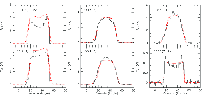
Figure 11: Best-fit model spectra for the different CO transitions to the available set of data at offset (0^′′,0^′′) for IK Tau. Parameters used to calculate the best-fit theoretical predictions are given in Table 5. The $\mathrm{{}^{12}CO(1-0)}$ and $\mathrm{{}^{12}CO(2-1)}$ data are from Teyssier et al. (2006), where ^′pv^′ means the IRAM 30 m telescope in Pico Veleta. The model fits are shown by dotted lines.

Figure 12: Model fits with different input parameters to the set of data at offset (0^′′, 0^′′) for IK Tau. Left column shows variations in the inner radius: $0.1\times 10^{14}$ cm (dash-dotted line), $1\times 10^{14}$ cm (dashed line), $10\times 10^{14}$ cm (dotted line). Middle column shows variation in $T_{0}$: $30$ K (dash-dotted line), $40$ K (dashed line), $50$ K (dotted line). Right column shows variations in the outer radius: $5.3\times 10^{16}$ cm (dash-dotted line), $6.3\times 10^{16}$ cm (dashed line), $7.3\times 10^{16}$ cm (dotted line) .

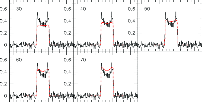
Figure 13: Model fits of the $\mathrm{{}^{13}CO}$(3-2) transition with different values for $T_{0}$, as indicated in the upper left corner of each panel. The model fits are shown by dotted lines.

4.2 Chemical abundance structure

As explained in the introduction, the density distribution of each molecule is different, depending on the chemical processes partaking in the envelope. The fractional abundance of a species A is usually specified as

$$f_{\mathrm{A}}(r)=\frac{n_{\mathrm{A}}(r)}{n_{\mathrm{H_{2}}}(r)}\,,$$ (8)

where $n_{\mathrm{H_{2}}}(r)$ is the number density of $\mathrm{H_{2}}$ and $n_{\mathrm{A}}(r)$ is the number density of species A.

A first order assessment of the molecular abundance fractions can be obtained assuming that the envelope structure is in local thermodynamic equilibrium. Assuming a spherically symmetric envelope, the fractional abundance for an optically thin rotational line ($J\rightarrow J-1$) of a linear rotor is given by Olofsson et al. (1991).

$$f_{x} = 3.8\times 10^{-16}T_{\mathrm{MB}}\frac{V^{2}_{\mathrm{exp}}BD}{\dot{M}}\frac{T_{\mathrm{ex}}}{\mu^{2}_{0}B^{2}_{0}J^{2}}$$ (9)

$$\cdot\exp(\frac{h(B_{0}\times 10^{9})J(J+1)}{kT_{\mathrm{ex}}})\frac{1}{\int^{x_{e}}_{x_{i}}\exp(-4\ln{2}x^{2})dx}$$

where $T_{\mathrm{MB}}$ is the main-beam brightness temperature, $T_{\mathrm{ex}}$ is the excitation temperature (= $T_{\mathrm{rot}}$ and equal to the kinetic temperature under the LTE assumption), $\mu_{0}$ is the dipole moment in Debye, $B_{0}$ is the rotational constant in GHz, $V_{\mathrm{exp}}$ is the gas expansion velocity of the CSE in $\mathrm{km\,s^{-1}}$, $B$ is the beam size in arcseconds, $D$ is the distance to the source in pc, $\dot{M}$ is the mass-loss rate in $\mathrm{M_{\odot}\,yr^{-1}}$, and $x_{i}$ (=0) and $x_{e}$ are the inner and outer radius of the CSE, respectively, measured in units of $B$. It has for simplicity been assumed that $f_{x}$ is constant from $x_{i}$ to $x_{e}$ and zero elsewhere. For CN, the relative strenghts of the different hyperfine components where taken into account. If the line is optically thick, the value of $f_{x}$ estimated by the above formula is only a lower limit.

The $\mathrm{SO_{2}}$ abundance with respect to $\mathrm{H_{2}}$ is estimated using the equation given by Morris et al. (1987):

$$f_{\mathrm{SO_{2}}} = \frac{T_{\mathrm{a}}(\mathrm{SO_{2}})}{2\times 10^{13}}\frac{V_{\mathrm{exp}}^{2}BDQ(T_{\mathrm{ex}})}{\dot{M}\mu_{0}^{2}S\nu}$$ (10)

$$\cdot\frac{1}{\exp[-1.44E_{\mathrm{u}}/T_{\mathrm{ex}}]}\frac{1}{\int^{x_{e}}_{x_{i}}\exp(-4\ln{2}x^{2})dx}$$

where $Q(T_{\mathrm{ex}})$ is the molecular partition function ($\simeq$ $1.15T_{\mathrm{ex}}^{3/2}$, for more detail see Omont et al. (1993)), $E_{\mathrm{u}}$ is the energy of the upper state of the transition, $S$ is the line strength, and $\nu$ is the frequency of the transition.

A mass loss rate of $\dot{M}=4.7\times 10^{-6}$ $\mathrm{{M_{\odot}\,yr^{-1}}}$ (see Sect. 4.1, and Teyssier et al. 2006) was adopted to calculate the abundances. Since the outer radius of the molecular emitting region can be quite uncertain for molecules for which no observational maps exist, two different outer radii will be used for these molecules (‘case A’ and ‘case B’). For SiO, the value for the outer radius was taken to be $2\times 10^{15}$ cm (case A) and $5\times 10^{15}$ cm (case B), for the other molecules $1\times 10^{16}$ cm (case A) and $5\times 10^{16}$ cm (case B) was assumed (Bujarrabal et al. 1994). For all lines from this work, we adopted expansion velocities from Table 4. For lines taken from the literature (see Table 7), an expanding velocity of 18 $\mathrm{km\,s^{-1}}$ is used consistent with our non-LTE CO modeling of the envelope. For the excitation temperatures, $T_{\mathrm{ex}}$, rotational temperatures as computed from Boltzmann diagrams are taken (see Table 6). Values for the upper energy level and line strength ($\mu_{0}^{2}S$) can be found in Table 4.

4.2.1 Results

Using the method outlined above, the fractional abundances of all molecules (except CO) were determined (see Table 7) .

Table 6: Rotational temperature and beam averaged column density.

Species	Trot (K)	N (cm-2)
SiS	85.8 (11.1)	4.46$\times$1015 (1$\times$1015)
SiO	17.1 (1.0)	8.24$\times$1015 (1$\times$1015)
SO	27.2 (2.7)	6.35$\times$1015 (2$\times$1015)
SO2	67.5 (6.8)	2.02$\times$1016 (4$\times$1015)
30SiO	68.6 (82.3)	2.48$\times$1014 (4$\times$1014)
29SiO	30.0 (15.5)	7.12$\times$1014 (9$\times$1014)
CS	33.9 (4.7)	8.89$\times$1014 (2$\times$1014)
HCN	8.3 (0.5)	2.27$\times$1015 (5$\times$1014)

Table 7: Derived molecular fractional abundance for each transition.

Species	Transition	Abundance	Outer radius	Abundance	Outer radius	Reference
		(case A)	(case A)	(case B)	(case B)
SiS	(5-4)	1.5$\times$10-6	1$\times$10${}^{16}\mathrm{cm}$	3.8$\times$10-7	5$\times$10${}^{16}\mathrm{cm}$	(1)
	(16-15)	6.0$\times$10-7		1.7$\times$10-7
	(17-16)	1.2$\times$10-6		3.6$\times$10-7
	(19-18)	1.3$\times$10-6		4.2$\times$10-7
	(20-19)	1.7$\times$10-6		5.4$\times$10-7
SiO	(2-1)	1.7$\times$10-5	2$\times$10${}^{15}\mathrm{cm}$	6.7$\times$10-6	5$\times$10${}^{15}\mathrm{cm}$	(1)
	(3-2)	1.5$\times$10-5		6.2$\times$10-6		(1)
	(5-4)	3.8$\times$10-6		1.5$\times$10-6		(2)
	(7-6)	8.3$\times$10-6		3.3$\times$10-6
	(8-7)	1.9$\times$10-5		7.6$\times$10-6
SO	(22-11)	2.0$\times$10-7	1$\times$10${}^{16}\mathrm{cm}$	5.2$\times$10-8	5$\times$10${}^{16}\mathrm{cm}$	(2)
	(56-45)	1.1$\times$10-6		4.3$\times$10-7		(1)
	(77-66)	2.3$\times$10-7		6.6$\times$10-8
	(88-77)	1.6$\times$10-6		5.1$\times$10-7
SO2	(31 3-20 2)	1.7$\times$10-5	1$\times$10${}^{16}\mathrm{cm}$	4.3$\times$10-6	5$\times$10${}^{16}\mathrm{cm}$	(2)
	(101 9-100 10)	1.1$\times$10-5		2.9$\times$10-6		(2)
	(100 10-91 9)	1.6$\times$10-5		5.1$\times$10-6		(2)
	(33 1-22 0)	6.0$\times$10-6		1.7$\times$10-6
	(171 17-160 16)	4.7$\times$10-5		1.4$\times$10-5
	(43 1-32 2)	4.8$\times$10-6		1.5$\times$10-6
	(132 12-121 11)	2.1$\times$10-5		6.5$\times$10-6
	(53 3-42 2)	2.5$\times$10-6		8.0$\times$10-7
	(144 10-143 11)	3.8$\times$10-6		1.2$\times$10-6
30SiO	(7-6)	2.2$\times$10-6	2$\times$10${}^{15}\mathrm{cm}$	8.7$\times$10-7	5$\times$10${}^{15}\mathrm{cm}$
	(8-7)	6.7$\times$10-6		2.8$\times$10-6
29SiO	(7-6)	6.2$\times$10-6	2$\times$10${}^{15}\mathrm{cm}$	2.5$\times$10-6	5$\times$10${}^{15}\mathrm{cm}$
	(8-7)	1.1$\times$10-5		4.6$\times$10-6
CS	(2-1)	4.7$\times$10-7	1$\times$10${}^{16}\mathrm{cm}$	1.1$\times$10-7	5$\times$10${}^{16}\mathrm{cm}$	(3)
	(3-2)	1.9$\times$10-7		5.9$\times$10-8		(1)
	(6-5)	3.2$\times$10-7		9.2$\times$10-8
	(7-6)	2.0$\times$10-7		6.3$\times$10-8
HCN	(1-0)	4.9$\times$10-7	1$\times$10${}^{16}\mathrm{cm}$	1.3$\times$10-7	5$\times$10${}^{16}\mathrm{cm}$	(1)
	(4-3)	2.3$\times$10-6		7.2$\times$10-7
CN	N=3-2, J=5/2-3/2	9.8$\times$10-8	1$\times$10${}^{16}\mathrm{cm}$	3.1$\times$10-8	5$\times$10${}^{16}\mathrm{cm}$
	N=3-2, J=7/2-5/2	2.3$\times$10-7		7.1$\times$10-8

(1) Bujarrabal et al. (1994); (2) Omont et al. (1993); (3) Lindqvist et al. (1988).

The most uncertain parameters used to derive the fractional abundances are $T_{\mathrm{ex}}$, $D$ and $x_{e}$ (the outer radius). $T_{\mathrm{ex}}$ is obtained from the rotational diagram analysis, $D$ is taken from the literature, and the outer radius of $x_{e}$ has been adopted differently for each individual molecule. We also note that our analysis assumes optically thin emission, which is not always the case for the studied line profiles. The line opacity is expected to be larger for higher $J$ rotational transitions, so that lower $J$ rotational transitions are expected to better probe the fractional abundance.

5 Discussion

Table 8: Comparison of the derived molecular fractional abundances with other published results.

	CS	HCN	SiO	SiS	SO	SO2	CN
This work (case A)	3.0$\times$10-7	1.4$\times$10-6	1.3$\times$10-5	1.3$\times$10-6	7.8$\times$10-7	1.4$\times$10-5	1.6$\times$10-7
This work (case B)	8.1$\times$10-8	4.3$\times$10-7	5.1$\times$10-6	3.7$\times$10-7	2.7$\times$10-7	4.2$\times$10-6	5.1$\times$10-8
(1)	1.0$\times$10-7	9.8$\times$10-7	1.7$\times$10-5	4.4$\times$10-7	2.6$\times$10-6	-	-
(2)	3.0$\times$10-7	6.0$\times$10-7	-	7.0$\times$10-7	-	-	-
(3)	-	-	3.0$\times$10-6	-	1.8$\times$10-6	4.1$\times$10-6	-
(4)	2.9$\times$10-7	1.4$\times$10-7	3.2$\times$10-5	3.5$\times$10-6	9.1$\times$10-7	2.2$\times$10-7	$3\times 10^{-7}$
(5)	2.8$\times$10-7	2.1$\times$10-6	3.8$\times$10-5	3.8$\times$10-10	7.8$\times$10-8	-	$2.4\times 10^{-10}$

(1) Bujarrabal et al. (1994); (2) Lindqvist et al. (1988); (3) Omont et al. (1993); (4) Willacy & Millar (1997); (5) Duari et al. (1999).

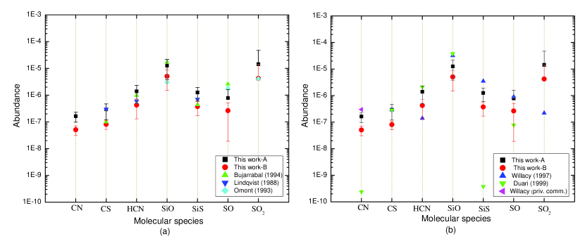
Figure 14: Comparison of the molecular fractional abundances derived in this work (case A and case B-study) and values found in literature (Bujarrabal et al. 1994; Lindqvist et al. 1988; Omont et al. 1993; Willacy & Millar 1997; Duari et al. 1999). The errors are estimated from the abundance variations for the different transitions (see Table 8). Panel (a) gives a comparison to other observational results, panel (b) to chemical model predictions.

Table 8 and Fig. 14 compare the average abundance of each molecule to values found in literature. Compared to observational results from literature (Bujarrabal et al. 1994; Lindqvist et al. 1988; Omont et al. 1993), our deduced fractional abundances agree within a factor of 3.5 for the smaller outer radius (case A) and for the larger outer radius (case B) within a factor of 10. Compared to the predicted abundances from theoretical chemical models by Willacy & Millar (1997) and Duari et al. (1999), we found that the predictions are comparable to our deduced values (using the smaller outer radius, case A) within a factor of $\sim$3 for $\mathrm{CS}$ and $\mathrm{SiO}$. Our deduced value for the SO, SiO, CN, and SiS fractional abundances agree with the results of Willacy & Millar (1997), but the predicted values by Duari et al. (1999) are much lower. The $\mathrm{SO_{2}}$ abundance from this work is almost two orders of magnitude higher than the value predicted by Willacy & Millar (1997).

As noted above, the SiS abundance in the chemical models of Duari et al. (1999) is much lower than the observed value. The chemical models by Duari et al. (1999) focus on the inner envelope (within few stellar radii), while Willacy & Millar (1997) studied the chemical processes partaking in the outer envelope. The agreement between our deduced value for the fractional abundance of SiS and the predictions by Willacy & Millar (1997) suggests that SiS is formed in the outer envelope.

The deduced SO abundance is a factor $\sim$10 higher than the inner wind predictions by Duari et al. (1999), but agree with the outer wind predictions by Willacy & Millar (1997). Willacy & Millar (1997) assumed no SO injection, but only in-situ formation. CN is clearly produced in the outer envelope, as photo-dissociation product of HCN.

The abundance of $\mathrm{SO_{2}}$ found by Willacy & Millar (1997) is much lower than the observed ones. A value of $1.4\times 10^{-5}$ (case A) means that SO₂ contains 80 % of the solar sulphur value. Willacy & Millar (1997) suggest that SO₂ may be formed in a different part of the envelope compared to the other sulphur bearing molecules, for example in shocks in bipolar outflow or in the inner envelope. An indication for the typical behavior of $\mathrm{SO_{2}}$ comes also from the line profiles, e.g. the $\mathrm{SO_{2}}$ (14–14) line is clearly narrower and shifted to the red.

The SiO abundance derived in this study is close to the abundance predicted by the theoretical chemical models. Cherchneff (2006) investigated the non-equilibrium chemistry of the inner winds of AGB stars and derived an almost constant, high SiO abundance (about $4\times 10^{-5}$ before the condensation of dust). Duari et al. (1999) and Willacy & Millar (1997) derived $3.8\times 10^{-5}$ and $3.2\times 10^{-5}$ for the inner and outer wind, respectively. Furthermore, González Delgado et al. (2003) performed an extensive radiative transfer analysis of circumstellar SiO emission from a large sample of M-type AGB stars, where they adopted the assumption that the gas-phase SiO abundance stays high close to the star, and further out the SiO molecular abundance fraction decreases due to absorption onto dust grains. Their results show that the derived abundances are always below the abundances expected from stellar atmosphere equilibrium chemistry. For a mass-loss rate of $4\times 10^{-6}$ M_⊙/yr, the equilibrium chemistry abundance of SiO is $\sim$3.5$\times 10^{-5}$ (Cherchneff 2006). Taking the scenario of depletion due to dust formation into account, the higher excitation SiO(8-7) would probe a higher SiO abundance. As seen in Table 7, the SiO(8-7) indeed probes a higher fractional abundance, although not significantly higher than the other lines.

6 Conclusions

In this work, we present for the (sub)millimeter survey for an oxygen-rich evolved AGB star, being IK Tau, in order to study the chemical composition in the envelope around the central target.

An extensive non-LTE radiative transfer analysis of circumstellar CO was performed using a model with a power law structure in temperature and density and a constant expansion. The observed line profiles of $\mathrm{{}^{12}CO(3-2)}$, $\mathrm{{}^{13}CO(3-2)}$, $\mathrm{{}^{12}CO(4-3)}$, and $\mathrm{{}^{12}CO(7-6)}$ are fit very well by our model, yielding a mass-loss rate of $4.7\times 10^{-6}$ M_⊙/yr. The line shapes and intensities for all $\mathrm{{}^{12}CO}$ transitions are not much influenced by variations of the inner radius, which is understandable since the bulk of the $\mathrm{{}^{12}CO}$ emission is produced in the outer envelope. The intensities for the higher excitation CO lines depend strongly on the assumed temperature but not on the value of the outer radius.

For 7 other molecules (SiO, SiS, HCN, CS, CN, SO, and SO₂) a fractional abundance study based on the assumption of LTE is performed. A full non-LTE analysis of all molecules is out of the scope of this observational paper, but will be presented in a next paper (Decin et al. 2010). This study shows that IK Tau is a good laboratory to study the conditions in circumstellar envelopes around oxygen-rich stars with submillimeter-wavelength molecular lines. The improved abundance estimates of this study will allow refinements of the chemical models in the future.

Molecular line modeling predicts the abundance of each molecule as a function of radial distance from the star, although some ambiguity about an inner or outer wind formation process often exists. To get a clear picture on the different chemistry processes partaking in the different parts in the envelope, mapping observations for molecules other than CO should be performed. Since most of the submillimeter emission from molecules less abundant than CO probably arises from the inner part of the envelope at 2 – 4^′′ meaningful observations require interferometers such as the future Atacama Large Millimeter Array (ALMA).