Quark-nucleon dynamics and Deep Virtual Compton Scattering

Abstract

We consider deeply virtual Compton scattering and deep inelastic scattering in presence of Regge exchanges that are part of the non-perturbative quark-nucleon amplitude. In particular we discuss contribution from the Pomeron exchange and demonstrate how it leads to Regge scaling of the Compton amplitude. Comparison with HERA data is given.

I Introduction

In the past two decades, notable theoretical activity has been dedicated to the study of the generalized parton distributions (GPD’s) ji1 ; radyushkin1 ; goeke ; belitsky ; diehl ; ji2 . GPD’s allow one to access the nucleon structure in a more detailed manner than the parton distribution functions (PDF’s) studied within DIS paradigm, and are a direct generalization of the latter. To access GPD’s, it was proposed to study hard exclusive processes like deeply virtual Compton scattering, (DVCS) $e+p\to e+p+\gamma$ ji3 ; radyushkin2 or meson electroproduction, $e+p\to e+p+\rho,\omega$, at high virtuality $Q^{2}$ of the photon originating from the scattered lepton, and low momentum transfer $t$ between recoiled and target nucleon. At present DVCS has been studied experimentally at HERA h1 ; h1_2 ; zeus ; zeus2 and Jefferson Lab clas1 ; clas2 . Interpretability of hard exclusive processes in terms of the GPD’s that are universal objects for all such reaction, is empowered by the collinear factorization theorem collins1 ; collins2 that, similarly as for DIS, allows for a separation of the soft hadronic amplitude from perturbative, QCD process with the former leading to four GPD’s. To the lowest order in the QCD coupling, $\alpha_{s}$, the full amplitude then corresponds to the handbag diagram depicted in Fig. 1. Paratactical applications, however, rest upon, the a priori unknown rate of convergence of the perturbative expansion. At low Bjorken-$x_{B}$ QCD corrections to the handbag diagram involve large logarithms in both $\alpha_{s}\log Q^{2}$ and $\alpha_{s}\log 1/x_{B}$. While significant progress has been made in devising various resumation schemes Fadin:1975cb ; Balitsky:1978ic ; Lipatov:1976zz ; Ciafaloni:1987ur ; Catani:1989yc ; Catani:1989sg ; Kwiecinski:1997ee , to date no first principle solution for the scattering amplitude exists. It is also accepted that the natural physical interpretation of the low-$x_{B}$ DIS is quite different from that of parton model description of the valence region dipole1 ; dipole2 ; dipole3 ; kopelyovich ; Stasto:2000er ; Brodsky:2002ue ; Brodsky:2004hi . That many orders in the $\alpha_{s}$ expansion may been needed to describe the low-$x_{B}$ region is consistent with the ample evidence that in exclusive electroproduction nonperturbative phenomena play an important role in the nominally perturbative domain. The structure functions at low-$x_{B}$ have the behavior characteristic to Pomeron and Regge phenomena, while at fixed momentum transfer, exclusive photon or meson electroproduction cross sections can be well fitted in terms of simple functions of $Q^{2}$ and the center of mass energy, $W$ rather then $Q^{2}$ and $x_{B}$ donnachie-dosch ; Donnachie:2000rz ; jenkovszky .

Recently we have proposed a model in which the diffractive phenomena that are expected to govern the low-$x_{B}$ DIS are incorporated at the parton nucleon level adam-tim ; adam . As discussed above, at the QCD side, at low-$x_{B}$ resumation of gluon ladders leads to complicated evolutions equations. However since at large center of mass energy, hadronic amplitudes are known to have a universal Regge scaling, we employ this phenomena to construct an effective parton-nucleon amplitude. In terms of the QCD description of  collins1 ; collins2 , in the model an infinite class of diagrams, i.e. those shown on the left panel in Fig. 2 is absorbed into the definition of the parton-nucleon blob and the resulting electroproduction amplitude is then computed from the handbag diagram. The model originates from a study of Regge phenomena at the parton level in the context of DIS Landshoff:1970ff ; Brodsky:1973hm . Such effective parton-nucleon amplitude gives the correct description of low-x structure functions, surprisingly, however, we have found that in the case of DVCS it breaks collinear factorization, i.e. Bjorken scaling while it naturally leads to the Regge-type scaling adam-tim ; adam . Upon closer examination, breaking of collinear approximation is not unexpected since it rests upon the assumption that parton-nucleon amplitude is a soft function of the invariant parton-nucleon energy, $\hat{s}$. This is not the case if the amplitude has Regge-type, $\hat{s}^{\alpha}$, $\alpha>0$ dependence on $\hat{s}$. Such Regge-type scaling of exclusive amplitudes at large $Q^{2}$ and all $x_{B}$ as opposed to Bjorken-scaling was in fact predicted by Bjorken and Kogut in  Bjorken:1973gc .

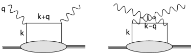
Figure 1: Handbag diagram representation of the Compton amplitude

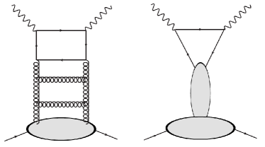
Figure 2: Infinite class of perturbative gluon ladders (left) is expected to lead to Regge phenomena and are absorbed into the quark-nucleon amplitude (right).

In this paper we focus on applicability of the the model to DVCS in the HERA kinematics, $Q^{2}/W^{2}<<1$. For description of HERA data on DVCS at low-$x$ two competing formalisms are used, Regge models that operate with the soft and hard Pomeron trajectories, as for example in the color dipole and similar models dipole1 ; dipole2 ; dipole3 ; kopelyovich ; kopelyovich ; donnachie-dosch ; Donnachie:2000rz ; jenkovszky , and the GPD-based models. To be applied phenomenologically, the GPD-based models would include models for Regge-like background, see e.g. polyakov-guzey ; lech ; polyakov-2 . In general Regge background thus represents a systematic effect on the extraction of GPD’s. Since both kinds of models are more or less successful in describing the HERA DVCS data, a question arises on whether the extraction of the GPD’s is model independent. Moreover, if data allow for interpretation without GPD’s, as in the model we study or the color dipole models, one may question the physical content of all these models.

The paper is organized as follows. In the following section we discuss the DVCS amplitude in the handbag approximation and emerging properties of the parton-nucleon amplitude based on Regge phenomenology. Computation of the DIS an DVCS amplitudes is discussed in Sec. III with more details included in the Appendix. Results and comparison with HERA data are presented in Sec. IV and followed by summary and conclusions in Sec. V.

II Compton amplitude in the handbag approximation

The hadronic Compton tensor is given by the matrix element of the time-ordered product of two electromagnetic currents,

$$T^{\mu\nu}=i\int d^{4}ze^{i\frac{q+q^{\prime}}{2}z}\langle N|T[J^{\nu}(z/2)J^{\mu}(-z/2)]|N\rangle$$

where $q(q^{\prime})$ is the four momentum of the incoming (outgoing) photon. We will consider both the DIS process that corresponds to the forward virtual Compton scattering with both photons spacelike, $q=q^{\prime}$, $q^{2}=q^{\prime 2}\equiv-Q^{2}<0$, and DVCS with $q^{2}<0,\;q^{\prime 2}=0$ and $\Delta=q-q^{\prime}\neq 0$. The currents are given by $J^{\mu}(z)=\sum_{q}e_{q}J_{q}^{\mu}(z),\;J_{q}^{\mu}(z)=\bar{\psi}_{q}(z)\gamma^{\mu}\psi_{q}(z)$ with $\psi_{q}$ the quark field operator and $e_{q}$ the quark charge. Using the leading order operator product expansion we replace the product of the two currents by the product of two quark field operators and a free quark propagator between the photon interaction points $z/2$ and $-z/2$, see Fig. 1 In this (handbag) approximation the hadronic Compton amplitude is then given by a convolution

$$T^{\mu\nu} = i\int\frac{d^{4}K}{(2\pi)^{4}}t^{\mu\nu}_{\alpha\beta}(K,q,\delta)A_{\alpha\beta}(K,\Delta,p,\lambda,\lambda^{\prime})$$ (2)

of the quark Compton tensor

$$t^{\mu\nu}_{\alpha\beta}(K,q,\delta)=$$ (3)

$$-e_{q}^{2}\left[\frac{\gamma^{\nu}(\displaystyle{\not}K+\frac{\displaystyle{\not}\,q+\displaystyle{\not}\,q^{\prime}}{2})\gamma^{\mu}}{\left(K+\frac{q+q^{\prime}}{2}\right)^{2}+i\epsilon}+\frac{\gamma^{\mu}(\displaystyle{\not}K-\frac{\displaystyle{\not}\,q+\displaystyle{\not}\,q^{\prime}}{2})\gamma^{\nu}}{\left(K-\frac{q+q^{\prime}}{2}\right)^{2}+i\epsilon}\right]_{\alpha\beta},$$

$\alpha,\beta$ being the Dirac indices, and the untruncated, with respect to the parton legs, parton-nucleon amplitude,

$$A_{\alpha\beta}(K,\Delta,p,\lambda,\lambda^{\prime})$$

$$=-i\int d^{4}ze^{-iKz}\langle p^{\prime}\lambda^{\prime}|T[\bar{\psi}_{\alpha}(z/2)\psi_{\beta}(-z/2)|p\lambda\rangle.$$ (4)

Following Brodsky:1973hm ; adam , we represent this amplitude as

$$A_{\alpha\beta}(K,\Delta,p,\lambda,\lambda^{\prime})=\int\frac{d\mu^{2}}{(k^{\prime 2}-\mu^{2}+i\epsilon)(k^{2}-\mu^{2}+i\epsilon)}$$

$$\times\sum_{i}\left[(\displaystyle{\not}k\,^{\prime}+\mu)\Gamma_{i}^{q}(\displaystyle{\not}k\,+\mu)\right]_{\alpha\beta}\bar{u}(p^{\prime})\Gamma_{i}^{N}u(p)$$ (5)

where $\Gamma_{i,j}^{q,N}$ are constructed from Dirac $\gamma$-matrices and the available four-vectors $p,\Delta,k$. The amplitude in Eq.(5) gives the correct result in perturbation theory, e.g. for point-like quark-nucleon interaction. For partons bound inside the nucleon, however, $A$ is expected to be suppressed at large-$k^{2}$ or $k^{\prime 2}$. This is achieved  Brodsky:1973hm ; adam , by applying to $A$ a generic operator Brodsky:1973hm $I_{n}=(\mu^{2})^{n}\left(\frac{d}{d\mu^{2}}\right)^{n}$, so that in Eq.(5),

$$\frac{1}{(k^{\prime 2}-\mu^{2}+i\epsilon)(k^{2}-\mu^{2}+i\epsilon)}$$

$$\to I_{n}\frac{1}{(k^{\prime 2}-\mu^{2}+i\epsilon)(k^{2}-\mu^{2}+i\epsilon)}.$$ (6)

This method of softening the UV behavior guarantees current conservation. This would not be the case, for example, if the two propagators were absorbed into a soft quark-nucleon wave function. Furthermore, differentiating the product of two propagators instead of differentiating each one separately ensures that the amplitude contains simple poles that enable to interpolate between the off- and on-shell quark-nucleon amplitudes.

II.1 Quark-nucleon amplitude with Regge behavior

We proceed by constructing the basis for the scattering process $N(p)+q(-k)\to N(p^{\prime})+q(-k^{\prime})$ shown in Fig.3.

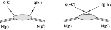
Figure 3: Direct and crossed contributions to the $quark-nucleon$-scattering amplitude

We account for all possible Dirac-Lorentz structures that can appear in four fermion operators. Furthermore we shall only consider those amplitudes which conserve the quark helicity since helicity-flip amplitudes are suppressed when integrated over in the handbag diagram by a power of $\mu/W$. The structures of interest thus involve $\sim\gamma^{\mu},\gamma^{\mu}\gamma_{5}$ on the quark side only. Based on $P$, $CP$ and $CPT$ invariance, the quark-nucleon scattering amplitude can be decomposed in the basis of six independent tensors each then multiplied by a Lorentz scalar function, $a_{i}$, $i=1,\dots 6$,

$$A_{qN} = \bar{q}\gamma^{\alpha}q\,\bar{N}\left[a_{1}\gamma_{\alpha}+a_{2}\frac{i\sigma_{\alpha\beta}\Delta^{\beta}}{2M}\right]N+a_{3}\bar{q}\gamma^{\alpha}\gamma_{5}q\,\bar{N}\gamma_{\alpha}\gamma_{5}N+\bar{q}\frac{\displaystyle{\not}K}{M}q\,\bar{N}\left[a_{4}+a_{5}\frac{\displaystyle{\not}K}{M}\right]N+\bar{q}\frac{\displaystyle{\not}\Delta\gamma_{5}}{2M}q\,\bar{N}\frac{\displaystyle{\not}\Delta\gamma_{5}}{2M}Na_{6},$$ (7)

were the new four-vectors are defined by, $K=(k+k^{\prime})/2$, $P=(p+p^{\prime})/2$, and $\Delta=k^{\prime}-k=p^{\prime}-p$. The amplitudes $a_{i}$ are analytic functions of invariants $\hat{s}=(p-k)^{2}=(P-K)^{2}$, $\hat{u}=(p^{\prime}+k^{\prime})^{2}=(P+K)^{2}$ and $t=\Delta^{2}$, fixed by the condition $\hat{s}+\hat{u}+t=2M^{2}+2\mu^{2}$ where $\mu$ is the mass of the effective quarks (c.f. Eq.(5)) and we have explicitly put the quarks on the mass shell. The above basis is equivalent to the form used in jamarcguichon for elastic electron-proton scattering. In particular the amplitude multiplying $a_{3}$ is chosen to be an axial vector but can be expressed in therms of $\bar{q}\displaystyle{\not}Pq\bar{N}\displaystyle{\not}KN$ used in jamarcguichon . Moreover, $\displaystyle{\not}\Delta\gamma_{5}/2M$ in front of $a_{6}$ becomes proportional to $\gamma_{5}$ for on-shell particles, whereas $\displaystyle{\not}K/M$ multiplying $a_{4}$ and $a_{5}$ reduces to $\mu/M$.

The scalar amplitudes $a_{i}$ have unitarity cuts in $\hat{s}$ and $\hat{u}$ and at fixed-$t$ can be represented through a dispersion representation,

$$a_{i}(\hat{s},\hat{u},t,\mu^{2}) = (2\pi)^{4}\int ds\left[\frac{\rho_{i}^{s}(s,t,\mu^{2})}{s-\hat{s}-i\epsilon}+\frac{\rho_{i}^{u}(s,t,\mu^{2})}{s-\hat{u}-i\epsilon}\right]$$ (8)

$$+\;{\rm subtractions}$$

with the spectral function $\rho_{i}^{s,u}$ being non-zero above some threshold values $s_{0}(u_{0})$ in the respective channel. Next, we consider the phenomenological consequences of Regge exchanges on the asymptotics of the spectral functions at high $s(u)$. For fixed $t$, we assume that the on-shell quark-nucleon helicity amplitudes follow Regge asymptotics, ${\it i.e.}$ they are proportional to $\hat{s}^{\alpha(t)}$ or $\hat{u}^{\alpha(t)}$ for large $\hat{s}$ or $\hat{u}$ respectively, $\alpha(t)$ being a Regge trajectory. Evaluating the asymptotic behavior of the amplitudes in Eq.(7) and comparing with the expected behavior in the Regge limit we find the asymptotic behavior of the spectral functions,

$$\rho_{1}^{u,s} \sim s^{\alpha_{1}-1}$$

$$\rho_{2}^{u,s} \sim s^{\alpha_{2}}$$

$$\rho_{3}^{u,s} \sim s^{\alpha_{3}-1}$$

$$\rho_{4}^{u,s} \sim s^{\alpha_{4}}$$

$$\rho_{5}^{u,s} \sim s^{\alpha_{5}-1}$$

$$\rho_{6}^{u,s} \sim s^{\alpha_{6}}$$ (9)

Note that in the pure collinear kinematics $\Delta^{\mu}=(\Delta^{+},0,0_{\perp})$ (thus for $\Delta^{2}=0$), and for massless quarks and proton, the matrix elements at $a_{2,4,6}$ vanish identically. Therefore, they generally have to be proportional to masses $M,\mu$ or momentum transfer $\Delta^{2}$ that is kept constant in Regge limit, and the above relations follow.

An additional constraint on the behavior of the spectral functions comes from the Pomeranchuk theorem which implies that asymptotically $s$ and $u$ channel amplitudes become equal. The $\hat{s}-\hat{u}$ crossing is implemented on the level of the quark-nucleon amplitudes according to

$$K \to -K$$

$$\Delta \to \Delta$$

$$\gamma^{\alpha} \to {\cal{C}}\gamma^{\alpha}{\cal{C}}^{\dagger}=-\gamma^{\alpha}$$

$$\gamma^{\alpha}\gamma^{5} \to {\cal{C}}\gamma^{\alpha}\gamma^{5}{\cal{C}}^{\dagger}=+\gamma^{\alpha}\gamma^{5},$$ (10)

with $C$ denoting the charge transformation. For the spectral functions in Eq.(7) Pomeranchuk’s theorem then implies,

$$\rho^{u}_{i}(s\to\infty) = +\rho^{s}_{i}(s\to\infty)\;\;\;\;{\rm for}\;\;i=3,4,6,$$

$$\rho^{u}_{i}(s\to\infty) = -\rho^{s}_{i}(s\to\infty)\;\;\;\;{\rm for}\;\;i=1,2,5.$$ (11)

We next introduce the $C$-even and $C$-odd combinations $\rho_{i}^{\pm}\equiv(\rho_{i}^{s}\pm\rho_{i}^{u})/2$ which asymptotically behave as,

$$\rho_{1}^{-}\sim s^{\alpha_{1}-1} \rho_{1}^{+}\sim s^{\alpha_{1}-2},$$

$$\rho_{2}^{-}\sim s^{\alpha_{2}} \rho_{2}^{+}\sim s^{\alpha_{2}-1},$$

$$\rho_{3}^{+}\sim s^{\alpha_{3}-1} \rho_{3}^{-}\sim s^{\alpha_{3}-2},$$

$$\rho_{4}^{+}\sim s^{\alpha_{4}} \rho_{4}^{-}\sim s^{\alpha_{4}-1},$$

$$\rho_{5}^{-}\sim s^{\alpha_{5}-1} \rho_{5}^{+}\sim s^{\alpha_{5}-2},$$

$$\rho_{6}^{+}\sim s^{\alpha_{6}} \rho_{6}^{-}\sim s^{\alpha_{6}-1}.$$ (12)

We notice that $\rho_{i}^{-}$ and $\rho_{i}^{+}$ correspond to singlet (valence + sea) and non-singlet (valence) GPD’s, respectively. It is instructive to observe that according to Eq.(12), only singlet combinations may grow with $s$ in the high energy regime, while the non-singlet ones necessarily vanish at high $s$. This fact, trivial in itself since it simply incorporates the symmetry of the interaction of the nucleon with highly energetic quark and antiquark, has important consequence for collinear factorization.

In Eq.(8), convergence of the dispersion integral at high energies is governed by asymptotic energy dependence of $\rho_{i}^{+}/s$ and $\rho_{i}^{-}/s^{2}$. Combining Eqs.(12),(8), it follows that one can at most expect three subtraction constants, for $a_{2}$, $a_{4}$ and $a_{6}$ footnote . The appearance of a finite subtraction constant that is energy-independent and thus has no exponential $t$-dependence would necessarily imply an appearance of fixed poles with very mild $t$-dependence in nucleon-nucleon and hadron-nucleon scattering. As it was noticed long ago Brodsky:1973hm ; brodsky-subconst , the experimental data do not support such possibility and we will assume in the following that these subtraction constants are zero.

The Pomeron can only contribute to the amplitude $a_{1}$. The amplitude $a_{3}$ has quantum numbers of an axial vector $a_{1}$-meson exchange which has the intercept $\alpha_{a_{1}}(0)\approx 0.5$ and needs no subtraction. The amplitude $a_{5}$ is crossing-odd and needs no subtraction.

III Regge exchange contribution to DIS and DVCS

In this section, we will employ handbag formalism and relate the quark-nucleon spectral functions $\rho_{i}^{\pm}$ to singlet and non-singlet GPD’s. We combine Eqs.(2),(3),(5), (8) to obtain the representation for the hadronic Compton amplitude

$$T^{\mu\nu}=i\int d\mu^{2}ds\int d^{4}K\sum_{i}\bar{u}(p^{\prime})\Gamma_{i}^{N}u(p)$$

$$\times\left[\frac{\rho_{i}^{s}}{s-(P-K)^{2}+i\epsilon}+\frac{\rho_{i}^{u}}{s-(P+K)^{2}+i\epsilon}\right]$$

$$\times I_{n}\frac{Tr\left[(\displaystyle{\not}K+\frac{\displaystyle{\not}\Delta}{2}+\mu)t^{\mu\nu}(\displaystyle{\not}K-\frac{\displaystyle{\not}\Delta}{2}+\mu)\Gamma_{i}^{q}\right]}{[(K+\Delta/2)^{2}-\mu^{2}+i\epsilon][(K-\Delta/2)^{2}-\mu^{2}+i\epsilon]}$$

(13)

Next, we will evaluate the contribution to the hadronic Compton amplitude from quark-nucleon amplitude proportional to $a_{1}$, i.e. use $\bar{u}(p^{\prime})\Gamma^{N}_{i}u(p)\Gamma^{q}_{i}=\bar{u}(p^{\prime})\gamma_{\alpha}u(p)\gamma^{\alpha}$ ($i=1$). This amplitude corresponds to Pomeron (and vector meson) exchange, so it should give the dominant contribution for DVCS at high energies where DVCS data from H1 and ZEUS are available, We choose the kinematics kinem as $p^{\mu}=(p^{+},0,0_{\perp})$ and $q^{\mu}=(0,Q^{2}/(2x_{B}p^{+}),Q_{\perp})$, with the usual Bjorken variable $x_{B}=Q^{2}/2pq$. The trace in Eq.(13) can be evaluated using the collinear approximation

$${\rm Tr}(\displaystyle{\not}k\,^{\prime}+\mu)t^{\mu\nu}(\displaystyle{\not}k+\mu)\gamma^{\alpha}\to-4g_{\perp}^{\mu\nu}(k_{\perp}^{2}+\mu^{2})\frac{Q^{2}}{2x_{B}P^{+}}g^{\alpha+}$$

$$\times\left[\frac{1}{(K+\frac{q+q^{\prime}}{2})^{2}+i\epsilon}-\frac{1}{(K-\frac{q+q^{\prime}}{2})^{2}+i\epsilon}\right],$$ (14)

Note that the above trace calculation in collinear kinematics is the same for forward (DIS) and non-forward (DVCS) case. Before we proceed, we notice that the trace in Eq.(14) is antisymmetric under exchanging $K\to-K$. This implies that only $\rho^{-}$ spectral density contributes leading to,

$$T^{\mu\nu}_{a_{1}} = -4ig_{\perp}^{\mu\nu}\frac{Q^{2}}{x_{B}}\frac{1}{2P^{+}}\bar{u}(p^{\prime})\gamma^{+}u(p)\int d\mu^{2}ds\int d^{4}KI_{n}\frac{k_{\perp}^{2}+\mu^{2}}{[(K+\Delta/2)^{2}-\mu^{2}+i\epsilon][(K-\Delta/2)^{2}-\mu^{2}+i\epsilon]}$$ (15)

$$\times \rho_{1}^{-}(s)\left[\frac{1}{s-(P-K)^{2}+i\epsilon}-\frac{1}{s-(P+K)^{2}+i\epsilon}\right]\left[\frac{1}{(K+\frac{q+q^{\prime}}{2})^{2}+i\epsilon}-\frac{1}{(K-\frac{q+q^{\prime}}{2})^{2}+i\epsilon}\right].$$

The fact that the above Compton amplitude depends on the singlet spectral function $\rho_{1}^{-}$ only, is independent of the collinear approximation: the positive $C$-parity of the Compton amplitude requires the $C$-even singlet combination $\rho_{1}^{-}$. On the contrary, the form factor, possessing the odd $C$-parity only depends on the $C$-odd non-singlet combination $\rho_{1}^{+}$.

III.1 DIS ($\gamma^{*}p\to\gamma^{*}p$)

We next evaluate the amplitude of Eq.(15) in the forward kinematics $\Delta=0$, $q^{2}=q^{\prime 2}=-Q^{2}$.

$$T^{\mu\nu}_{a_{1}}(\Delta=0)=-4ig_{\perp}^{\mu\nu}\frac{Q^{2}}{x_{B}}\frac{1}{2p^{+}}\bar{u}(p^{\prime})\gamma^{+}u(p)$$

$$\times\int d\mu^{2}ds\int d^{4}kI_{n}\frac{k_{\perp}^{2}+\mu^{2}}{(k^{2}-\mu^{2}+i\epsilon)^{2}}\rho_{1}^{-}(s)$$

$$\times\left[\frac{1}{s-(p-k)^{2}+i\epsilon}-\frac{1}{s-(p+k)^{2}+i\epsilon}\right]$$

$$\times\left[\frac{1}{(k+q)^{2}+i\epsilon}-\frac{1}{(k-q)^{2}+i\epsilon}\right].$$ (16)

We make the collinear approximation in the hard quark propagators,

$$\frac{1}{(k+q)^{2}+i\epsilon}\approx\frac{1}{-Q^{2}+\frac{Q^{2}}{x_{B}p^{+}}k^{+}+i\epsilon}=\frac{x_{B}/Q^{2}}{\frac{k^{+}}{p^{+}}-x_{B}+i\epsilon},$$

$$\frac{1}{(k-q)^{2}+i\epsilon}\approx\frac{1}{-Q^{2}-\frac{Q^{2}}{x_{B}p^{+}}k^{+}+i\epsilon}=\frac{-x_{B}/Q^{2}}{\frac{k^{+}}{p^{+}}x_{B}-i\epsilon},$$

(17)

and obtain (we refer to the Appendix A for more details),

$$T^{\mu\nu}(\Delta=0) = -4\pi^{2}g_{\perp}^{\mu\nu}\frac{1}{2p^{+}}\bar{u}(p^{\prime})\gamma^{+}u(p)\Gamma(n)\int_{0}^{1}dx(1-x)^{n+1}\int d\mu^{2}(\mu^{2})^{n}ds\rho_{1}^{-}(s,t=0,\mu^{2})\frac{(n+1-x)\mu^{2}+xs}{[-(1-x)\mu^{2}-xs]^{n+1}}$$ (18)

$$\times \int dk^{+}\left[\frac{1}{\frac{k^{+}}{p^{+}}-x_{B}+i\epsilon}+\frac{1}{\frac{k^{+}}{p^{+}}+x_{B}-i\epsilon}\right]\left[\delta(k^{+}-xp^{+})-\delta(k^{+}+xp^{+})\right]$$

To make a connection to the PDF’s, we consider the imaginary part of this amplitude. Recalling that the imaginary part of forward Compton tensor proportional to $-g^{\mu\nu}$ gives $\pi W_{1}\to\pi\frac{1}{2}\sum_{q}e_{q}^{2}[q(x)-\bar{q}(-x)]$, we identify the parton densities with integrals over the $\rho^{-}$ or explicitly $s$ and $u$ spectral functions as,

$$x_{B}[q(x_{B})-\bar{q}(-x_{B})]=-8\pi^{2}\Gamma(n)(-1)^{n+1}(1-x_{B})^{n+1}$$

$$\times\int d\mu^{2}d\xi(\mu^{2})^{n}[\rho_{1}^{s}(\frac{\xi}{x_{B}},0,\mu^{2})-\rho_{1}^{u}(-\frac{\xi}{x_{B}},0,\mu^{2})]$$

$$\times\frac{\xi+(n+1-x_{B})\mu^{2}}{(\xi+(1-x_{B})\mu^{2})^{n+1}}.$$ (19)

In the above, we changed the integration variable $s$ to $\xi=x_{B}s$. Using the high energy asymptotics (c.f. Eq.(9)) $\rho_{1}^{s,u}(s)\sim s^{\alpha_{P}-1}$, with $\alpha_{P}=1+\epsilon$ being the Pomeron trajectory, and pull the $x_{B}$ dependence out of the $\xi$-integral we obtain the experimentally observed asymptotics $F_{2}(x_{B})\sim x_{B}^{1-\alpha_{P}}\sim x_{B}^{-\epsilon}$. This is the result for the singlet PDF. The non-singlet combination will depend on a similar integral with the non-singlet spectral function, which at high energy behaves as $\rho^{+}(s)\sim s^{\alpha_{P}-2}$, and correspondingly gives $x_{B}[q(x_{B})+\bar{q}(-x_{B})]\sim x_{B}^{2-\alpha_{P}}\sim x_{B}$, as expected. Evaluating the real part of the forward Compton amplitude we obtain the familiar result for DIS,

$$T^{\mu\nu}(\Delta=0) = g_{\perp}^{\mu\nu}\frac{1}{2p^{+}}\bar{u}(p^{\prime})\gamma^{+}u(p)$$

$$\times \int_{0}^{1}dx\frac{2x}{x^{2}-x_{B}^{2}+i\epsilon}[q(x)-\bar{q}(-x)].$$

While the singlet PDF’s at low $x$ rise as $x^{-\alpha_{P}}$, the singularity at $x\to 0$ is cancelled by one power of $x$ in the numerator of Eq.(LABEL:limit) which makes both the imaginary and real part of the integral finite adam .

III.2 DVCS ($\gamma^{*}p\to\gamma p$): collinear approximation

Next we evaluate Eq.(15) in the DVCS kinematics, $p^{\mu}=(p^{+},0,0_{\perp})$, $q^{\mu}=(0,Q^{2}/(2x_{B}p^{+}),Q_{\perp})$, $\Delta^{\mu}=(-x_{B}p^{+},0,0_{\perp})$, and choose now asymmetric integration variable $k$, rather than $K=\frac{k+k^{\prime}}{2}$,

$$T^{\mu\nu}_{a_{1}} = -4ig_{\perp}^{\mu\nu}\frac{Q^{2}}{x_{B}}\frac{1}{2p^{+}}\bar{u}(p^{\prime})\gamma^{+}u(p)\int d\mu^{2}ds\int d^{4}k(k_{\perp}^{2}+\mu^{2})I_{n}\frac{1}{[k^{2}-\mu^{2}+i\epsilon][(k+\Delta)^{2}-\mu^{2}+i\epsilon]}$$ (21)

$$\times \rho_{1}^{-}(s)\left[\frac{1}{s-(p-k)^{2}+i\epsilon}-\frac{1}{s-(p+k+\Delta)^{2}+i\epsilon}\right]\left[\frac{1}{(k+q)^{2}+i\epsilon}-\frac{1}{(k-q^{\prime})^{2}+i\epsilon}\right],$$

Using the collinear approximation for the quark propagator exchanged between the two photons interaction points we obtain in the case of DVCS,

$$\frac{1}{(k+q)^{2}+i\epsilon}\approx\frac{1}{-Q^{2}+\frac{Q^{2}}{x_{B}p^{+}}k^{+}+i\epsilon}=\frac{x_{B}/Q^{2}}{\frac{k^{+}}{p^{+}}-x_{B}+i\epsilon},$$

$$\frac{1}{(k-q^{\prime})^{2}+i\epsilon}\approx\frac{1}{-\frac{Q^{2}}{x_{B}p^{+}}k^{+}+i\epsilon}=\frac{x_{B}/Q^{2}}{-\frac{k^{+}}{p^{+}}+i\epsilon}.$$ (22)

The DVCS amplitude in the collinear approximation is then given by,

$$T^{\mu\nu}_{a_{1}} = g_{\perp}^{\mu\nu}\frac{1}{2P^{+}}\bar{u}(p^{\prime})\gamma^{+}u(p)$$

$$\times \int_{0}^{1}dx\left[\frac{1}{x-x_{B}+i\epsilon}+\frac{1}{x-i\epsilon}\right]H^{+}(x,x_{B}),$$

and we refer the reader to the Appendix B for the details of the calculation. We identify the singlet GPD $H(x,x_{B})$ with,

$$H^{+}(x,x_{B}) = (1-x_{B}/2)\int_{0}^{1}dy\int_{0}^{1}dz[q(z)-\bar{q}(-z)]$$ (24)

$$\times \delta(x-z-yx_{B}(1-z))$$

which satisfies the familiar normalization condition,

$$\int_{0}^{1}dxH^{+}(x,x_{B}) = (1-x_{B}/2)\int_{0}^{1}dx[q(x)-\bar{q}(-x)].$$

The factor $(1-x_{B}/2)$ in the definition of the GPD results from the prefactor $1/2P^{+}$ in the DVCS amplitude. Unlike DIS, in the presence of Regge asymptotics, the real part of the integral in Eq.(LABEL:HC) is divergent. This can be seen by first integrating the $\delta$-function over $x$, and then performing the integral over $y$. In the limit $z\to 0$ the real part of the integral

$$\int_{0}^{1}dy\left[\frac{1}{z-x_{B}+yx_{B}(1-z)+i\epsilon}+\frac{1}{z+yx_{B}(1-z)-i\epsilon}\right]$$ (26)

is finite, and equal to $\ln(1-x_{B})/x_{B}$ Then, given the Regge asymptotics of the PDF, $[q(z)-\bar{q}(-z)]\sim z^{-\alpha_{P}}$ the integral over $z$ diverges. In the case of the DIS amplitude the quark propagator exchanged between the two photons in the sum of direct and crossed handbag diagram (c.f. Fig. 1) leads to the factor of $x$ in the numerator of Eq.(LABEL:limit). This does not happen in DVCS when one photon is soft and the sum of the two collinear propagators in the DVCS amplitude of Eq.(LABEL:HC) does not vanish when $x\to 0$ and cannot compensate for the rise of the GPD at low $x$. We also note that in the case of the non-singlet GPD, the integral over $x$ instead reduces to $\sim dxx^{1-\alpha_{P}}$ and is therefore convergent. Thus conclude that for valence GPD’s where Regge contributions are suppressed the collinear approximation is adequate and that part of the full DVCS amplitude would obey Bjorken scaling. As we show in the following section, inclusion of Regge contributions into singlet GPD’s leads to Regge scaling.

III.3 DVCS beyond the collinear approximation

We will use the collinear approximation in the numerator only. We combine all four propagators together using Feynman parameters to obtain

$$T^{\mu\nu}=-8ig_{\perp}^{\mu\nu}\frac{Q^{2}}{x_{B}}\frac{1}{2p^{+}}\bar{u}\gamma^{+}u\int d\mu^{2}I_{n}\int ds\rho_{1}^{-}(s)\Gamma(4)\int_{0}^{1}dxdydz(1-x)(1-z)^{2}$$ (27)

$$\times\int d^{4}k\left[\frac{k_{\perp}^{2}+\mu^{2}}{([k+zq-(1-z)xp+y(1-x)(1-z)\Delta]^{2}-z(1-z)Q^{2}(1-x/x_{B}-y(1-x))-(1-z)[xs+(1-x)\mu^{2}])^{4}}\right.$$

$$\;\;\;\;\;\;\left.-\frac{k_{\perp}^{2}+\mu^{2}}{([k-zq^{\prime}-(1-z)xp+y(1-x)(1-z)\Delta]^{2}-z(1-z)Q^{2}(x/x_{B}+y(1-x))-(1-z)[xs+(1-x)\mu^{2}])^{4}}\right]$$

We report all the details of the algebra in the Appendix C, and quote here the final result,

$$T^{\mu\nu} = 8\pi^{2}g_{\perp}^{\mu\nu}\frac{(Q^{2})^{\alpha-1}}{x_{B}^{\alpha}}\frac{1}{2p^{+}}\bar{u}\gamma^{+}u\int d\mu^{2}\mu^{4}I_{n-2}\int d\xi\xi^{\alpha-1}\int_{0}^{Q^{2}/x_{B}}\frac{d\omega}{\omega^{\alpha-1}}\left(1-\frac{x_{B}}{Q^{2}}\omega\right)^{2}\beta_{1}^{-}\left(\frac{Q^{2}\xi}{x_{B}\omega}\right)$$

$$\times \left\{-\frac{\xi+3\mu^{2}}{[\xi+\mu^{2}]^{3}}\frac{1}{\omega}\ln\left[\frac{|\xi+\mu^{2}-\omega(1-x_{B})|}{\xi+\mu^{2}+\omega}\frac{\xi+\mu^{2}+Q^{2}+\omega(1-x_{B})}{|\xi+\mu^{2}+Q^{2}-\omega|}\right]\right.$$

$$+\frac{2\mu^{2}}{[\xi+(1-x)\mu^{2}]^{2}}\left[\frac{2-x_{B}}{[\xi+\mu^{2}-\omega(1-x_{B})][\xi+\mu^{2}+\omega]}-\frac{2-x_{B}}{[\xi+\mu^{2}+Q^{2}+\omega(1-x_{B})][\xi+\mu^{2}+Q^{2}-\omega]}\right]$$

$$\left.+2\frac{\mu^{2}+Q^{2}}{\xi+\mu^{2}}\left[\frac{(2-x_{B})(\xi+\mu^{2}+\omega x_{B}/2)}{[\xi+\mu^{2}-\omega(1-x_{B})]^{2}[\xi+\mu^{2}+\omega]^{2}}-\frac{(2-x_{B})(\xi+\mu^{2}+Q^{2}-\omega x_{B}/2)}{[\xi+\mu^{2}+Q^{2}+\omega(1-x_{B})]^{2}[\xi+\mu^{2}+Q^{2}-\omega]^{2}}\right]\right\},$$

where we changed variables from $s$ to $\xi=xs$, from $x$ to $\omega=Q^{2}x/x_{B}$, and factored out the Regge asymptotics of the spectral function as $\rho_{1}^{-}(s)=s^{\alpha-1}\beta_{1}^{-}(s)$ with $\beta\to const.$ for $s\to\infty$. Analyzing the above formula, we notice that integrals now converge. Importantly, large values of $\omega$ do not contribute to the integral because of the explicit suppression factor $(1-x_{B}\omega/Q^{2})^{2}$ and because of powers of $\omega$ in the denominator inside the bracket. The price to pay for this convergence is the appearance of the explicit scale dependence $\sim\mu^{2}$ in the expressions, as compared to the scale-independent results obtained within the collinear approximation. This scale dependence is of no surprise since Regge behavior does introduce a scale. In the limit $Q^{2}/\mu^{2}>>1$ it can be shown that the leading contribution of the Pomeron, $\alpha=\alpha_{P}$ to this integral is proportional to

$$T_{DVCS}\sim\frac{1}{Q^{2}}\left(\frac{Q^{2}}{x_{B}}\right)^{\alpha_{P}}\sim\frac{W^{2\alpha_{P}}}{Q^{2}}.$$ (29)

In the following Section, we will confront this parametrization with the DVCS data.

IV Results and Comparison with HERA data

The result of the previous section, for $T_{DVCS}$ was obtained in the limit $Q^{2}\to\infty$ at finite $Q^{2}$ the amplitude is finite but would require knowledge of the spectral decomposition of the quark-nucleon amplitude at finite energies. When comparing to the experimental data at finite $Q^{2}$ we thus replace $1/Q^{2}$ by a $\sim 1/(1+Q^{2}/Q_{0}^{2})$ with some characteristic scale $Q_{0}^{2}$ that we will determine from a fit. This is in accord with the experimental observationh1

$$\sigma_{DVCS} = \sigma_{0}(W^{2})^{2\alpha-2}(Q^{2})^{\delta}$$ (30)

with $\delta\approx-1.5$ rather than $-2$. It is also this form that is used to describe data within phenomenological Regge (or color dipole picture-motivated) models donnachie-dosch ; jenkovszky . We will fit the HERA data using the following parametrization for the cross section

$$\sigma_{\gamma^{*}p\to\gamma p}=\sigma_{0}\left[\left(\frac{W}{W_{0}}\right)^{\alpha-1}\left(\frac{1}{1+Q^{2}/Q_{0}^{2}}\right)\right]^{2}$$ (31)

with $W_{0}=20\mbox{ GeV}$. It is worth noting that using the reggized parton-nucleon amplitude in the handbag model we have effectively ”derived” the parametrization proposed in donnachie-dosch ).

We perform two fits. One is a combined fit to both H1 h1 ; h1_2 and ZEUS zeus ; zeus2 data. It gives $\sigma_{0}=28\pm 4\mbox{ nb}$, $Q_{0}=1.51\pm 0.05\mbox{GeV}$ and $\alpha-1=0.43\pm 0.03$ and is shown in Figs 4, with $\chi^{2}/d.o.f.=2.01$.

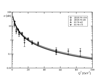
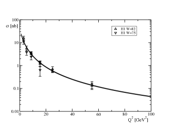
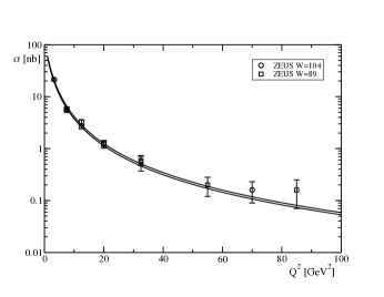
Figure 4: DVCS cross section as a function of photon virtuality, $Q^{2}$ for various c.m. energies $W$ (in GeV). In the upper panel, we confront the combined fit to the H1 and ZEUS data. Solid lines a result of a fit to the combined ZEUS and H1 data including both $Q^{2}$ and $W$ dependence. The middle panel displays a similar fit to H1 data alone, whereas the fits to ZEUS data alone are shown in the lower panel.

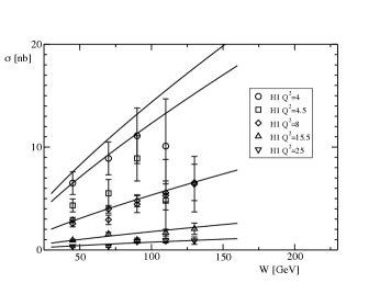
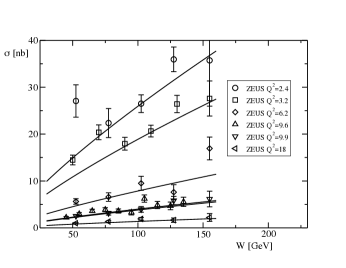
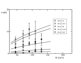
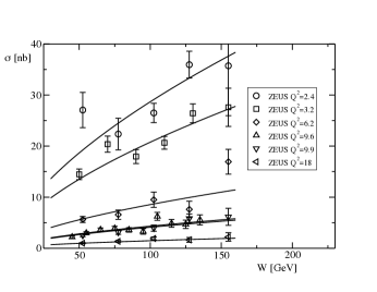
Figure 5: $W$-dependence of the DVCS cross section for different values of $Q^{2}$. The upper panel displays the comparison of the H1 data to the combined fit to both data sets, whereas the second panel from top shows the ZEUS data vs. the same fit. The two lower panels confront individual fits to H1 (second lowest panel) and ZEUS (lowest panel) to the corresponding data sets.

The other, is an independent fit to H1 and ZEUS data. For the fit to the H1 data alone we obtain $\sigma_{0}=17\pm 3\mbox{ nb}$, $Q_{0}=1.83\pm 0.1\mbox{GeV}$ and $\alpha-1=0.34\pm 0.05$ and it is shown in Figs 4, 5, with $\chi^{2}/d.o.f.=1.2$. For an independent fit to the ZEUS data alone we find $\sigma_{0}=41\pm 7\mbox{ nb}$, $Q_{0}=1.49\pm 0.06\mbox{GeV}$ and $\alpha-1=0.34\pm 0.03$ and it is shown in Figs 4, 5, with $\chi^{2}/d.o.f.=1.1$. We observe that both data sets are fitted well with the Regge form of Eq.(31), as it was found previously in color dipole or Regge based studies donnachie-dosch . However, the two data sets exhibit different normalization (the values of $\sigma_{0}$). As a result, performing a combined analysis we obtain a higher intercept.

V Summary

We presented an analysis of quark-nucleon scattering amplitudes. We considered a basis of six independent Dirac-Lorentz structures and discussed their Regge behavior. In particular we have shown that the $C$-odd combinations of the direct and crossed channels (referred to as non-singlet combinations) follow different Regge asymptotics, as compared to the $C$-even (singlet) ones. Once embedded into the handbag diagram to describe the DVCS amplitude in hard kinematics, we show that only singlet combinations contribute, whereas the valence combinations do not appear and require no a priori unknown subtractions.

We focused on the contribution of a single Pomeron trajectory that dominates at high energies, and have demonstrate that while for DIS the handbag formalism leads to the known result, $F_{2}(x_{B})\sim x_{B}^{-\alpha_{P}}$, in the case of DVCS, the mismatch between quark propagators leads to divergent integrals in the collinear approximation. If collinear approximation is not used, the model naturally leads to Regge-scaling for DVCS Bjorken:1973gc with $T_{DVCS}\sim Q^{(2\alpha_{P}-2)}/x_{B}^{\alpha_{P}}$, with $\alpha_{P}=1+\epsilon$ being the Pomeron trajectory. Thus we have reproduce the form that phenomenological Regge models use to describe DVCS, and we have illustrated its applicability by fitting the data from HERA. In he future we plan to extend our phenomenological analysis to larger values of Bjorken $x_{B}$, where DVCS was measured at Jefferson Lab clas1 ; clas2 . Since the JLab data is taken at much lower energies, however, the Pomeron trajectory alone is not expected to be sufficient and other trajectories will have to be studied.

Appendix A DIS in collinear approximation

Here we evaluate the forward Compton amplitude of Eq.(16),

$$T^{\mu\nu}_{a_{1}}(\Delta=0) = -4ig_{\perp}^{\mu\nu}\frac{Q^{2}}{x_{B}}\frac{1}{2p^{+}}\bar{u}(p^{\prime})\gamma^{+}u(p)\int d\mu^{2}ds\int d^{4}kI_{n}\frac{k_{\perp}^{2}+\mu^{2}}{(k^{2}-\mu^{2}+i\epsilon)^{2}}$$ (32)

$$\times \rho_{1}^{-}\left[\frac{1}{s-(p-k)^{2}+i\epsilon}-\frac{1}{s-(p+k)^{2}+i\epsilon}\right]\left[\frac{1}{(k+q)^{2}+i\epsilon}-\frac{1}{(k-q)^{2}+i\epsilon}\right].$$

Using the collinear quark propagators from Eq. (17) and introducing the Feynman parameter $x$, we obtain,

$$T^{\mu\nu}_{a_{1}} = 4ig_{\perp}^{\mu\nu}\frac{1}{2p^{+}}\bar{u}(p)\gamma^{+}u(p)\int d\mu^{2}ds\rho_{1}^{-}(s,\Delta^{2},\mu^{2})\int dk^{+}dk^{-}d^{2}k_{\perp}\left[\frac{1}{\frac{k^{+}}{p^{+}}-x_{B}+i\epsilon}+\frac{1}{\frac{k^{+}}{p^{+}}+x_{B}-i\epsilon}\right]$$ (33)

$$\times (k_{\perp}^{2}+\mu^{2})I_{n}\frac{1}{[k^{2}-\mu^{2}+i\epsilon]^{2}}\left[\frac{1}{(p-k)^{2}-s-i\epsilon}-\frac{1}{(p+k)^{2}-s-i\epsilon}\right]$$

$$= 4ig_{\perp}^{\mu\nu}\frac{1}{2P^{+}}\bar{u}(p^{\prime})\gamma^{+}u(p)\Gamma(n+3)\int_{0}^{1}dx(1-x)^{n+1}\int d\mu^{2}(\mu^{2})^{n}ds\rho_{1}^{-}(s,\Delta^{2},\mu^{2})$$

$$\times \int dk^{+}\left[\frac{1}{\frac{k^{+}}{p^{+}}-x_{B}+i\epsilon}+\frac{1}{\frac{k^{+}}{p^{+}}+x_{B}-i\epsilon}\right]$$

$$\times \int dk^{-}d^{2}k_{\perp}\left[\frac{(k_{\perp}^{2}+\mu^{2})}{[(k-yp)^{2}-ys-(1-y)\mu^{2}]^{n+3}}-\frac{(k_{\perp}^{2}+\mu^{2})}{[(k+yp)^{2}-ys-(1-y)\mu^{2}]^{n+3}}\right].$$

Finally, Eq.(18) is obtained from Eq. (33) after integrating over $k^{-},k_{\perp}$ using,

$$\int dk^{-}d^{2}k_{\perp}\frac{1}{(k^{2}+a^{2})^{\alpha}} = i\pi^{2}\frac{\Gamma(\alpha-2)}{\Gamma(\alpha)}\frac{\delta(k^{+})}{(a^{2})^{\alpha-2}}$$

$$\int dk^{-}d^{2}k_{\perp}\frac{k_{\perp}^{2}}{(k^{2}+a^{2})^{\alpha}} = -i\pi^{2}\frac{\Gamma(\alpha-3)}{\Gamma(\alpha)}\frac{\delta(k^{+})}{(a^{2})^{\alpha-3}}.$$

The expression in Eq.(18) follows from Eq.(33) after integrating over $k^{+}$.

Appendix B DVCS in collinear approximation

We evaluate Eq.(15) in the DVCS kinematics, $p^{\mu}=(p^{+},0,0_{\perp})$, $q^{\mu}=(0,Q^{2}/(2x_{B}p^{+}),Q_{\perp})$, $\Delta^{\mu}=(-x_{B}p^{+},0,0_{\perp})$, and use $k$ as the integration variable instead of $K=(k+k^{\prime})/2$,

$$T^{\mu\nu}_{a_{1}} = -4ig_{\perp}^{\mu\nu}\frac{Q^{2}}{x_{B}}\frac{1}{2p^{+}}\bar{u}(p^{\prime})\gamma^{+}u(p)\int d\mu^{2}ds\int d^{4}k(k_{\perp}^{2}+\mu^{2})I_{n}\frac{1}{[k^{2}-\mu^{2}+i\epsilon][(k+\Delta)^{2}-\mu^{2}+i\epsilon]}$$ (35)

$$\times \rho_{1}^{-}\left[\frac{1}{s-(p-k)^{2}+i\epsilon}-\frac{1}{s-(p+k+\Delta)^{2}+i\epsilon}\right]\left[\frac{1}{(k+q)^{2}+i\epsilon}-\frac{1}{(k-q^{\prime})^{2}+i\epsilon}\right].$$

We use the collinear approximation of Eq. (22) and combine the two quark propagators from the untruncated, quark-nucleon amplitude introducing an integral over a Feynman parameter,

$$\frac{1}{[k^{2}-\mu^{2}+i\epsilon][(k+\Delta)^{2}-\mu^{2}+i\epsilon]}=$$

$$=\int_{0}^{1}dy\frac{1}{[(k+y\Delta)^{2}-\mu^{2}+i\epsilon]^{2}},$$ (36)

to obtain,

$$T^{\mu\nu}_{a_{1}} = 4ig_{\perp}^{\mu\nu}\frac{1}{2p^{+}}\bar{u}(p^{\prime})\gamma^{+}u(p)\int_{0}^{1}dy\int d\mu^{2}ds\rho_{1}^{-}(s,\Delta^{2},\mu^{2})\int dk^{+}dk^{-}d^{2}k_{\perp}\left[\frac{1}{\frac{k^{+}}{p^{+}}-x_{B}+i\epsilon}-\frac{1}{-\frac{k^{+}}{p^{+}}+i\epsilon}\right]$$

$$\times (k_{\perp}^{2}+\mu^{2})I_{n}\frac{1}{[(k+y\Delta)^{2}-\mu^{2}+i\epsilon]^{2}}\left[\frac{1}{(p-k)^{2}-s-i\epsilon}-\frac{1}{(p+k+\Delta)^{2}-s-i\epsilon}\right]$$

$$= 4ig_{\perp}^{\mu\nu}\frac{1}{2p^{+}}\bar{u}(p^{\prime})\gamma^{+}u(p)\int_{0}^{1}dy\Gamma(n+3)\int_{0}^{1}dx(1-x)^{n+1}\int d\mu^{2}(\mu^{2})^{n}ds\rho_{1}^{-}(s,\Delta^{2},\mu^{2})$$

$$\times \int dk^{+}\left[\frac{1}{\frac{k^{+}}{p^{+}}-x_{B}+i\epsilon}-\frac{1}{-\frac{k^{+}}{p^{+}}+i\epsilon}\right]$$

$$\times \int dk^{-}d^{2}k_{\perp}\left[\frac{(k_{\perp}^{2}+\mu^{2})}{[(k-xp+y(1-x)\Delta)^{2}-xs-(1-x)\mu^{2}]^{n+3}}-\frac{(k_{\perp}^{2}+\mu^{2})}{[(k+xp^{\prime}+y(1-x)\Delta)^{2}-xs-(1-x)\mu^{2}]^{n+3}}\right]$$

Integrating over $k^{-},k_{\perp}$ results in

$$T^{\mu\nu}_{a_{1}} = -4\pi^{2}g_{\perp}^{\mu\nu}\frac{1}{2p^{+}}\bar{u}(p^{\prime})\gamma^{+}u(p)\int_{0}^{1}dy\Gamma(n)\int_{0}^{1}dx(1-x)^{n+1}\int d\mu^{2}(\mu^{2})^{n}ds\rho_{1}^{-}(s,\Delta^{2},\mu^{2})\frac{(n+1-x)\mu^{2}+xs}{[-(1-x)\mu^{2}-xs+i\epsilon]^{n+1}}$$

$$\times \int dk^{+}\left[\frac{1}{\frac{k^{+}}{p^{+}}-x_{B}+i\epsilon}-\frac{1}{-\frac{k^{+}}{p^{+}}+i\epsilon}\right]\left[\delta(k^{+}-(x+yx_{B}(1-x))p^{+})-\delta(k^{+}+(x(1-x_{B})-yx_{B}(1-x))p^{+})\right]$$

The argument of the second $\delta$-function can be brought to the same form of the first $\delta$-function by changing integration variables $y\to 1-y$ and $k^{+}\to-k^{+}+x_{B}p^{+}$. Finally, the result reads

$$T^{\mu\nu}_{a_{1}} = -4\pi^{2}g_{\perp}^{\mu\nu}\frac{1}{2p^{+}}\bar{u}(p^{\prime})\gamma^{+}u(p)\int_{0}^{1}dy\Gamma(n)\int_{0}^{1}dx(1-x)^{n+1}\int d\mu^{2}(\mu^{2})^{n}ds\rho_{1}^{-}(s,\Delta^{2},\mu^{2})\frac{(n+1-x)\mu^{2}+xs}{[-(1-x)\mu^{2}-xs+i\epsilon]^{n+1}}$$ (39)

$$\times 2\left[\frac{1}{x-x_{B}+yx_{B}(1-x)+i\epsilon}+\frac{1}{x+yx_{B}(1-y)-i\epsilon}\right]$$

which corresponds to Eq. (LABEL:HC) with $H$ defined in Eq.(24).

Appendix C DVCS beyond the collinear approximation

We use the collinear approximation in numerator of Eq.(13) and combine all four propagators using Feynman parameters,

$$T^{\mu\nu}=-8ig_{\perp}^{\mu\nu}\frac{Q^{2}}{x_{B}}\frac{1}{2p^{+}}\bar{u}\gamma^{+}u\int d\mu^{2}I_{n}\int ds\rho_{1}^{-}(s)\Gamma(4)\int_{0}^{1}dxdydz(1-x)(1-z)^{2}$$ (40)

$$\times\int d^{4}k\left[\frac{k_{\perp}^{2}+\mu^{2}}{([k+zq-(1-z)xp+y(1-x)(1-z)\Delta]^{2}-z(1-z)Q^{2}(1-x/x_{B}-y(1-x))-(1-z)[xs+(1-x)\mu^{2}])^{4}}\right.$$

$$\;\;\;\;\;\;\left.-\frac{k_{\perp}^{2}+\mu^{2}}{([k-zq^{\prime}-(1-z)xp+y(1-x)(1-z)\Delta]^{2}-z(1-z)Q^{2}(x/x_{B}+y(1-x))-(1-z)[xs+(1-x)\mu^{2}])^{4}}\right]$$

Integration over $d^{4}k$ results in

$$T^{\mu\nu} = 8\pi^{2}g_{\perp}^{\mu\nu}\frac{Q^{2}}{x_{B}}\frac{1}{2p^{+}}\bar{u}\gamma^{+}u\int d\mu^{2}\mu^{4}I_{n-2}\int ds\rho_{1}^{-}(s)\Gamma(3)\int_{0}^{1}dxdydz(1-x)^{3}$$

$$\times \left\{\frac{1-z}{[xs+(1-x)\mu^{2}+zQ^{2}(1-x/x_{B}-y(1-x))]^{3}}-\frac{1-z}{[xs+(1-x)\mu^{2}+zQ^{2}(x/x_{B}+y(1-x))]^{3}}\right.$$

$$\left.+\frac{3(\mu^{2}+z^{2}Q^{2})}{[xs+(1-x)\mu^{2}+zQ^{2}(1-x/x_{B}-y(1-x))]^{3}}-\frac{3(\mu^{2}+z^{2}Q^{2})}{[xs+(1-x)\mu^{2}+zQ^{2}(x/x_{B}+y(1-x))]^{3}}\right\}$$

Next the $y$ integral can be done to obtain,

$$T^{\mu\nu} = 8\pi^{2}g_{\perp}^{\mu\nu}\frac{1}{x_{B}}\frac{1}{2p^{+}}\bar{u}\gamma^{+}u\int d\mu^{2}\mu^{4}I_{n-2}\int ds\rho_{1}^{-}(s)\Gamma(3)\int_{0}^{1}dx(1-x)^{2}\frac{dz}{z}$$

$$\times \left\{(1-z)\left[\frac{1}{[xs+(1-x)\mu^{2}+zQ^{2}(x-x/x_{B})]^{2}}-\frac{1}{[xs+(1-x)\mu^{2}+zQ^{2}(1-x/x_{B})]^{2}}\right.\right.$$

$$\left.+\frac{1}{[xs+(1-x)\mu^{2}+zQ^{2}(1-x+x/x_{B})]^{2}}-\frac{1}{[xs+(1-x)\mu^{2}+zQ^{2}x/x_{B}]^{2}}\right]$$

$$+2(\mu^{2}+z^{2}Q^{2})\left[\frac{1}{[xs+(1-x)\mu^{2}+zQ^{2}(x-x/x_{B})]^{3}}-\frac{1}{[xs+(1-x)\mu^{2}+zQ^{2}(1-x/x_{B})]^{3}}\right.$$

$$\left.\left.+\frac{1}{[xs+(1-x)\mu^{2}+zQ^{2}(1-x+x/x_{B})]^{3}}-\frac{1}{[xs+(1-x)\mu^{2}+zQ^{2}x/x_{B}]^{3}}\right]\right\}$$

and finally $z$ integral yields,

$$T^{\mu\nu} = 8\pi^{2}g_{\perp}^{\mu\nu}\frac{1}{x_{B}}\frac{1}{2p^{+}}\bar{u}\gamma^{+}u\int d\mu^{2}\mu^{4}I_{n-2}\int d\xi\xi^{\alpha-1}\beta_{1}^{-}(\frac{\xi}{x})\int_{0}^{1}\frac{dx}{x^{\alpha}}(1-x)^{2}$$

$$\times \left\{-\frac{\xi+(3-x)\mu^{2}}{[\xi+(1-x)\mu^{2}]^{3}}\ln\left[\frac{\xi+(1-x)\mu^{2}+Q^{2}(x-x/x_{B})}{\xi+(1-x)\mu^{2}+Q^{2}x/x_{B}}\frac{\xi+(1-x)\mu^{2}+zQ^{2}(1-x+x/x_{B})}{\xi+(1-x)\mu^{2}+zQ^{2}(1-x/x_{B})}\right]\right.$$

$$+\frac{2\mu^{2}}{[\xi+(1-x)\mu^{2}]^{2}}\left[\frac{1}{\xi+(1-x)\mu^{2}+Q^{2}(x-x/x_{B})}-\frac{1}{\xi+(1-x)\mu^{2}+Q^{2}(1-x/x_{B})}\right.$$

$$\left.+\frac{1}{\xi+(1-x)\mu^{2}+Q^{2}(1-x+x/x_{B})}-\frac{1}{\xi+(1-x)\mu^{2}+Q^{2}x/x_{B}}\right]$$

$$+\frac{\mu^{2}+Q^{2}}{\xi+(1-x)\mu^{2}}\left[\frac{1}{[\xi+(1-x)\mu^{2}+Q^{2}(x-x/x_{B})]^{2}}-\frac{1}{[\xi+(1-x)\mu^{2}+Q^{2}(1-x/x_{B})]^{2}}\right.$$

$$\left.\left.+\frac{1}{[\xi+(1-x)\mu^{2}+Q^{2}(1-x+x/x_{B})]^{2}}-\frac{1}{[\xi+(1-x)\mu^{2}+Q^{2}x/x_{B}]^{2}}\right]\right\},$$

where we changed variables from $s$ to $\xi=xs$ and factored out the Regge asymptotics of the spectral function as $\rho_{1}^{-}(s)=s^{\alpha-1}\beta_{1}^{-}(s)$ with $\beta\to const.$ for $s\to\infty$. To proceed, we observe that the integral over $\xi$ is convergent since $\rho_{1}^{-}\sim\xi^{\alpha-1}$ and the expression in the curly bracket drops at least as $1/\xi^{3}$. Instead, the $x$ integral is peaked at $x\to 0$, and we can therefore neglect $x$ in terms proportional to $(1-x)$. The divergent behavior of this integral obtained in collinear approximation for the propagators can obtained the formal limit $Q^{2}\to\infty$ Then, the expression in the curly bracket becomes $Q^{2}$-independent, and proportional to $\sim\ln(1-x_{B})$ leading to a divergent integral of the type $\int_{0}dxx^{-\alpha}$. To ensure convergence, we do not make this approximation. Changing finally the integration variable $x$ to $\omega=Q^{2}x/x_{B}$, we obtain Eq.(III.3).

References

• (1) X.D. Ji, Phys. Rev. Lett. 78, 610 (1997).
• (2) A.V. Radyushkin, Phys. Rev. D 56, 5524 (1997).
• (3) X.D. Ji, J. Phys. G 24, 1181 (1998).
• (4) K. Goeke, M. V. Polyakov and M. Vanderhaeghen, Prog. Part. Nucl. Phys. 47, 401 (2001).
• (5) A. V. Belitsky, D. Mueller and A. Kirchner, Nucl. Phys. B 629, 323 (2002).
• (6) M. Diehl, Phys. Rept. 388, 41 (2003).
• (7) X. D. Ji, Phys. Rev. D 55, 7114 (1997).
• (8) A. V. Radyushkin, Phys. Lett. B 380, 417 (1996).
• (9) A. Aktas et al., [H1 Collaboration], Eur. Phys. J. C 44, 1 (2005).
• (10) F. D. Aaron et al. [H1 Collaboration], Phys. Lett. B 659, 796 (2008).
• (11) S.Chekanov et al. [ZEUS collaboration], Phys. Lett. B 573, 46 (2003).
• (12) S.Chekanov et al. [ZEUS collaboration], JHEP 05, 108 (2009).
• (13) S. Stepanyan et al. [CLAS Collaboration], Phys. Rev. Lett. 87, 182002 (2001).
• (14) S. Chen et al. [CLAS Collaboration], Phys. Rev. Lett. 97, 072002 (2006).
• (15) J.C. Collins, L. Frankfurt, M. Strikman, Phys. Rev. D 56, 2982 (1997).
• (16) J.C. Collins, A. Freund, Phys. Rev. D59, 074009 (1999).
• (17) V. S. Fadin, E. A. Kuraev and L. N. Lipatov, Phys. Lett.  B 60 (1975) 50.
• (18) I. I. Balitsky and L. N. Lipatov, Sov. J. Nucl. Phys.  28, 822 (1978) [Yad. Fiz.  28, 1597 (1978)].
• (19) L. N. Lipatov, Sov. J. Nucl. Phys.  23, 338 (1976) [Yad. Fiz.  23, 642 (1976)].
• (20) M. Ciafaloni, Nucl. Phys.  B 296, 49 (1988).
• (21) S. Catani, F. Fiorani and G. Marchesini, Phys. Lett.  B 234, 339 (1990).
• (22) S. Catani, F. Fiorani and G. Marchesini, Nucl. Phys.  B 336, 18 (1990).
• (23) J. Kwiecinski, A. D. Martin and A. M. Stasto, Phys. Rev.  D 56, 3991 (1997).
• (24) J. Nemchik, N. N. Nikolaev, E. Predazzi, and B. G. Zakharov, Z.Phys. C 75, (1997) 71.
• (25) K. Golec-Biernat and M. Wusthoff, Phys. Rev. D 59, (1999) 014017; Phys. Rev. D 60, (1999) 114023.
• (26) J. R. Forshaw, G. Kerley, and G. Shaw, Phys. Rev. D 60, (1999) 074012; Nucl. Phys. A 675, (2000) 80.
• (27) B.Z. Kopeliovich, I. Schmidt, M. Siddikov, Phys.Rev. D 79, 034019 (2009).
• (28) A. M. Stasto, K. J. Golec-Biernat and J. Kwiecinski, Phys. Rev. Lett.  86, 596 (2001).
• (29) S. J. Brodsky, P. Hoyer, N. Marchal, S. Peigne and F. Sannino, Phys. Rev.  D 65, 114025 (2002).
• (30) S. J. Brodsky, R. Enberg, P. Hoyer and G. Ingelman, Phys. Rev.  D 71, 074020 (2005).
• (31) A. Donnachie, H.G. Dosch, Phys.Lett. B 502, 74 (2001).
• (32) A. Donnachie, J. Gravelis and G. Shaw, Eur. Phys. J.  C 18, 539 (2001)
• (33) M. Capua, S. Fazio, R. Fiore, L. Jenkovszky, F. Paccanoni, Phys. Lett. B 645, 161 (2007).
• (34) A. P. Szczepaniak, J. T. Londergan and F. J. Llanes-Estrada, Acta Phys. Polon.  B 40, 2193 (2009).
• (35) A.P. Szczepaniak, T. Londergan, Phys. Lett. B 643, 17 (2006).
• (36) P. V. Landshoff, J. C. Polkinghorne and R. D. Short, Nucl. Phys.  B 28, 225 (1971).
• (37) S. J. Brodsky, F. E. Close and J. F. Gunion, Phys. Rev.  D 8, 3678 (1973).
• (38) J. D. Bjorken and J. B. Kogut, Phys. Rev.  D 8, 1341 (1973).
• (39) V. Guzey, M.V. Polyakov, Eur.Phys.J. C 46, 151 (2006).
• (40) L. Mankiewicz, G. Piller and A. Radyushkin, Eur. Phys. J. C 10, 307 (1999).
• (41) M. Penttinen, M. V. Polyakov and K. Goeke, Phys. Rev. D 62, 014024 (2000).
• (42) M. Gorchtein, P.A.M. Guichon, M. Vanderhaeghen, Nucl.Phys. A 741, 234 (2004).
• (43) In the case of $a_{2}$, the subtraction is only necessary if the Pomeron has a non-zero magnetic coupling to the nucleon. Pomeranchuk’s theorem rules out Pomeron contribution to spin-flipping amplitudes. The amplitude $a_{4}$ requires subtraction due to the $f_{2}$-exchange with positive Regge intercept. Finally, $a_{6}$ corresponds to $\pi$-trajectory exchange with intercept $\alpha_{\pi}(0)\approx 0$ and needs a subtraction. The amplitude $a_{5}$ is crossing-odd and needs no subtraction since the corresponding Dirac structure does not allow for a Pomeron contribution. However, a two-Pomeron exchange could contribute to this amplitude.
• (44) S. J. Brodsky, F. E. Close and J. F. Gunion, Phys. Rev.  D 6, 177 (1972).
• (45) We use notation $a^{\mu}=(a^{+},a^{-},a_{\perp})$ with $a^{\pm}=(a^{0}\pm a^{3})/\sqrt{2}$, thus $a_{\mu}b^{\mu}=a^{+}b^{-}+a^{-}b^{+}-\vec{a}_{\perp}\vec{b}_{\perp}$.