A modified semi–implicit Euler-Maruyama scheme for finite element discretization of SPDEs with additive noise

Abstract

We consider the numerical approximation of a general second order semi–linear parabolic stochastic partial differential equation (SPDE) driven by additive space-time noise. We introduce a new modified scheme using a linear functional of the noise with a semi–implicit Euler–Maruyama method in time and in space we analyse a finite element method (although extension to finite differences or finite volumes would be possible). We prove convergence in the root mean square $L^{2}$ norm for a diffusion reaction equation and diffusion advection reaction equation. We present numerical results for a linear reaction diffusion equation in two dimensions as well as a nonlinear example of two-dimensional stochastic advection diffusion reaction equation. We see from both the analysis and numerics that the proposed scheme has better convergence properties than the standard semi–implicit Euler–Maruyama method.

1 Introduction

We analyse the strong numerical approximation of Ito stochastic partial differential equations defined in $\Omega\subset\mathbb{R}^{d}$. Boundary conditions on the domain $\Omega$ are typically Neumann, Dirichlet or some mixed conditions. We consider equations of the form

$$dX=(AX+F(X))dt+dW,\qquad X(0)=X_{0},\qquad t\in[0,T],\quad T>0$$ (1)

in a Hilbert space $H=L^{2}(\Omega)$. Here $A$ is the generator of an analytic semigroup $S(t):=e^{tA},t\geq 0$ with eigenfunctions $e_{i}$ and eigenvalues $\lambda_{i}$, $i\in\mathbb{N}^{d}$. $F$ is a nonlinear function of $X$ and possibly $\nabla X$. The noise term, $W(x,t)$, is a $Q$-Wiener process that is white in time and defined on a filtered probability space $(\mathbb{D},\mathcal{F},\mathbb{P},\left\{F_{t}\right\}_{t\geq 0})$. We assume that the noise can be represented as

$$W(x,t)=\underset{i\in\mathbb{N}^{d}}{\sum}\sqrt{q_{i}}e_{i}(x)\beta_{i}(t),$$ (2)

where $q_{i}$, $i\in\mathbb{N}^{d}$ are respectively the eigenvalues and the eignfunctions of $Q$, and $\beta_{i}$ are independent and identically distributed standard Brownian motions. Precise assumptions on $A$, $F$ and $W$ are given in Section 3 and, under these type of technical assumptions, it is well known (see DaPZ ; PrvtRcknr ; Chw ) that the unique mild solution is given by

$$X(t)=S(t)X_{0}+\int_{0}^{t}S(t-s)F(X(s))ds+O(t)$$ (3)

with the stochastic process $O$ given by the stochastic convolution

$$O(t)=\int_{0}^{t}S(t-s)dW(s).$$ (4)

The study of numerical solutions of SPDEs is an active area of research and there is a growing literature on numerical methods for SPDEs (see allen98:_finit ; Lakkis ; KssrsZrrs ; GTambueexpoM ; Jentzen1 ; Jentzen2 ; Jentzen3 ; Jentzen4 and reference therein).

Our numerical scheme is built on recent work by Jentzen and co-workers Jentzen1 ; Jentzen2 ; Jentzen3 ; Jentzen4 that uses Taylor expansion and linear functionals of the noise for a spectral Fourier–Galerkin discretisations of (1) and obtained high order schemes in time. Let us describe briefly these schemes. Let $P_{N}$, $N\in\mathbb{N}$ be the spectral projection defined for $u\in L^{2}(\Omega)$ by

$$P_{N}u=\sum_{i\in\mathcal{I}_{N}}(e_{i},u)e_{i},\qquad\qquad\mathcal{I}_{N}=\left\{1,2,...,N\right\}^{d}.$$ (5)

The spectral Galerkin discretisation of (1) yields the following semi-discrete form

$$dX^{N}=(A_{N}X^{N}+F_{N}(X^{N}))dt+dW^{N},$$ (6)

with $A_{N}=P_{N}A,\;F_{N}=P_{N}F$ and $W^{N}=P_{N}W$ and is a diagonal system to solve for each Fourier mode. For time stepping we make use of the standard $\varphi-$functions

$$\varphi_{0}(\Delta tA_{N}) = e^{\Delta tA_{N}}$$ (7)

$$\varphi_{1}(\Delta tA_{N}) = (\Delta t\,A_{N})^{-1}\left(e^{\Delta tA_{N}}-I\right)=\frac{1}{\Delta t}\int_{0}^{\Delta t}e^{(\Delta t-s)A_{N}}ds.$$ (8)

Jentzen and co-workers Jentzen3 ; Jentzen4 examine the following two high order time stepping schemes which overcome the order barrier (see Jentzen3 ) of numerical schemes approximating (1)

$$X_{m+1}^{N}=e^{\Delta tA_{N}}X_{m}^{N}+\Delta t\varphi_{1}(\Delta tA_{N})F_{N}(X_{m}^{N})+P_{N}O_{m}$$ (9)

and

$$Y_{m+1}^{N}=\varphi_{0}(\Delta tA_{N})\left(Y_{m}^{N}+\Delta tF_{N}(Y_{m}^{N})\right)+P_{N}O_{m}.$$ (10)

The process

$$O_{m}=\int_{t_{m}}^{t_{m+1}}e^{\left(t_{m+1}-s\right)A}dW$$ (11)

has the exact variance in each Fourier mode as an Ornstein–Uhlenbeck process. More precisely, by assuming that the linear operator $A$ and the covariance operator $Q$ have the same eigenbasis, applying the Ito isometry in each mode yields

$$(e_{i},O_{m})=e^{-\lambda_{i}\Delta t}\left(\dfrac{q_{i}}{2\lambda_{i}}\left(1-e^{-2\lambda_{i}\Delta t}\right)\right)^{1/2}R_{i,m},$$ (12)

$i\in\mathcal{I}_{N}=\left\{1,2,3,...,N\right\}^{2}$, $m=0,1,2...,M-1$ and $R_{i,m}$ are independent, standard normally distributed random variables with means $0$ and variance $1$. In equation (12) the noise is termed to be computed using a linear functional.

Although schemes (9)-(10) are of higher order in time, these improved convergence rates were only established under seriously restrictive commutativity assumptions which exclude most nonlinear Nemytskii operators. This was recently overcome in xia . Another drawback is that to implement the schemes, the eigenfunctions of the linear operator $A$ and of the covarance operator $Q$ must coincide and furthermore must be known explicitly (see (12)). To illustrate that this can be overcome with our spatial discretisation we solve the SPDE

$$dX=\left(D\varDelta X-\nabla\cdot(\textbf{q}X)+R(X)\right)dt+dW,$$ (13)

on a rectangular domain with mixed boundary conditions without requiring information on the eigenvalues and eigenfunctions of the corresponding linear operator. The velocity $\mathbf{q}$ in (13) is obtained from the following steady state mass conservation equation and Darcy’s law

$$\nabla\cdot\mathbf{q}=0,\qquad\mathbf{q}=-\dfrac{\mathbf{k}}{\mu}\nabla p,$$ (14)

where $\mathbf{k}$ is the heterogeneous permeability tensor, $p$ is the pressure and $\mu$ is the dynamic viscosity of the fluid sebastianb . In (13), $R$ is the reaction function which may be a Langmuir adsorption term which is globally Lipschitz sebastianb and $D>0$ the diffusion coefficient. Typically (13)-(14) is solved using finite elements or finite volumes as spectral Galerkin approach is not infeasible due to the heterogeneous nature of the permeability and the fact that such problems often naturally give rise to non-uniform. Our work differs from other finite element discretisations allen98:_finit ; Lakkis ; KssrsZrrs ; GTambueexpoM where the noise is considered directly in the finite element space. We follow more closely Yn:04 ; Yn:05 ; Haus1 and introduce a projection onto a finite number modes and a projection onto the finite element space. The aim is to gain the flexibility of the finite element (finite volume) discretisation to deal with flow and transport problems (13)-(14), complex boundaries, mixed boundary conditions and inhomogeneous boundary conditions as well as reaching high order in time as in Jentzen3 ; Jentzen4 .

The paper is organised as follows. In Section 3 we present the numerical scheme and assumptions that we make on the linear operator, nonlinearity and the noise. We consider fairly weak conditions on nonlinear function $F$ as recently considered in xia . We then state and discuss our main results. These are convergence in the root mean square $L^{2}(\Omega)$ norm for reaction-diffusion equations and advection–reaction–diffusion for spatially regular noise. We present simulations in Section 4, these are applied both to a linear example where we can compute an exact solution as well as a more realistic model coming from model of the advection and diffusion of a solute in a porous media with a non-linear reaction term. We also show that, equipped with the eigenvalues and eigenfunctions of the operator $\varDelta$ with Neumann or Dirichlet boundary conditions, we can apply the new scheme with mixed boundary conditions without explicitly having the eigenvalues and eigenfunctions for this case. We present numerical results both for finite element and finite volume discretisations in space. Finally, in Section 5.2 and Section 5.3, we present the proofs of the convergence theorems for the finite element discretisation.

2 Setting and Assumptions

Let us start by presenting briefly the notation for the main function spaces and norms that we use in the paper. We denote by $\|\cdot\|$ the norm associated to the inner product $(\cdot,\cdot)$ of the $\mathbb{R}-$Hilbert space $H=L^{2}(\Omega)$. For a Banach space $\mathcal{V}$ we denote by $\|\cdot\|_{\mathcal{V}}$ the norm of the space $\mathcal{V}$, $L(\mathcal{V})$ the set of bounded linear mapping from $\mathcal{V}$ to $\mathcal{V}$, $L^{(2)}(\mathcal{V})$ the set of bounded bilinear mapping from $\mathcal{V}\times\mathcal{V}$ to $\mathbb{R}$ and $L_{2}(\mathbb{D},\mathcal{V})$ the Hilbert space of all equivalence classes of square integrable $\mathcal{V}-$valued random variables.

Let $Q:H\rightarrow H$ be a positive self adjoint operator, we consider throughout this work the $Q$-Wiener process. We denote the space of Hilbert–Schmidt operators from $Q^{1/2}(H)$ to $H$ by $L_{2}^{0}:=\mathcal{L}_{2}(Q^{1/2}(H),H)=HS(Q^{1/2}(H),H)$ and the corresponding norm $\|.\|_{L_{2}^{0}}$ by

$$\|l\,\|_{L_{2}^{0}}:=\|lQ^{1/2}\|_{\mathcal{L}_{2}(H)}=\left(\underset{i\in\mathbb{N}^{d}}{\sum}\|lQ^{1/2}e_{i}\|^{2}\right)^{1/2},\qquad\ l\in L_{2}^{0}.$$

Let $\varphi:[0,T]\times\Omega\rightarrow L_{2}^{0}$ be a $L_{2}^{0}-$valued predictable stochastic process with $\mathbb{P}\left[\int_{0}^{t}\|\varphi\|_{L_{2}^{0}}^{2}ds<\infty\right]=1,\,t\in[0,T]$. We have the following equality known as the Ito’s isometry

$$\mathbf{E}\|\int_{0}^{t}\varphi dW\|^{2}=\int_{0}^{t}\mathbf{E}\|\varphi\|_{L_{2}^{0}}^{2}ds=\int_{0}^{t}\mathbf{E}\|\varphi Q^{1/2}\|_{HS}^{2}ds.$$

Throughout the paper we assume that $\Omega$ is bounded and has a smooth boundary or is a convex polygon. For convenience of presentation we take $A$ to be a self adjoint second order operator as this simplifies the convergence proof. More precisely

$$A=\nabla\cdot\textbf{D}\nabla(.)+D_{0,0}\mathbf{I}=\underset{i,j=1}{\sum^{d}}\dfrac{\partial}{\partial x_{i}}\left(D_{i,j}\dfrac{\partial}{\partial x_{j}}\right)+D_{0,0}\mathbf{I},$$ (15)

where we assume that $D_{i,j}=D_{j,i}\in L^{\infty}(\Omega)$ and that there exists a positive constant $c_{1}>0$ such that

$$\underset{i,j=1}{\sum^{d}}D_{i,j}(x)\xi_{i}\xi_{j}\geq c_{1}|\xi|^{2}\;\;\;\;\;\;\forall\xi\in\mathbb{R}^{d}\;\;\;x\in\overline{\Omega}\;\;\;c_{1}>0.$$ (16)

The derivatives in (15) are understood in the sense of distributions (weak sense). We introduce two spaces $\mathbb{H}$ and $V$ where $\mathbb{H}\subset V$. These spaces depend on the choice of the boundary conditions and on the variational form associated to the operator $A$. For Dirichlet boundary conditions we let

$$V=\mathbb{H}=H_{0}^{1}(\Omega)=\{v\in H^{1}(\Omega):v=0\quad\text{on}\quad\partial\Omega\}.$$

For Robin boundary conditions (Neumann boundary condition being a particular case) we let $V=H^{1}(\Omega)$ and

$$\mathbb{H}=\left\{v\in H^{2}(\Omega):\partial v/\partial\nu_{A}+\sigma v=0\quad\text{on}\quad\partial\Omega\right\},\qquad\sigma\in\mathbb{R}.$$

Note that $\partial v/\partial\nu_{\mathcal{A}}$ is the normal derivative of $v$ and $\nu_{\mathcal{A}}$ is the exterior pointing normal $\mathbf{n}=(n_{i})$ to the boundary of $\Lambda$ given by

$$\partial v/\partial\nu_{\mathcal{A}}=\underset{i,j=1}{\sum^{d}}n_{i}(x)D_{i,j}(x)\dfrac{\partial v}{\partial x_{j}}.$$ (17)

Let $-A:\mathcal{D}(-A)\subset H\rightarrow H$ be the unbounded operator with domain $\mathcal{D}(-A)$. Under condition (16), it is well known (see lions ) that the linear operator $-A$ generates an analytic semigroup $S(t):=e^{tA}$. Functions in $\mathbb{H}$ can satisfy the boundary conditions. With the space $\mathbb{H}$ in hand we can characterize the domain of the operator $(-A)^{r/2}$ and have the following norm equivalence lions ; Stig ; ElliottLarsson for $r\in\{1,2\}$

$$C_{1}\|v\|_{H^{r}(\Omega)} \leq \|(-A)^{r/2}v\|\leq C_{2}\|v\|_{H^{r}(\Omega)}\,\,\qquad\forall\,\,v\in\mathcal{D}((-A)^{r/2}),$$

$$\mathcal{D}((-A)^{r/2}) = \mathbb{H}\cap H^{r}(\Omega)\,\,\qquad\qquad\qquad\quad\text{ (Dirichlet boundary conditions)},$$

$$\mathcal{D}((-A)) = \mathbb{H},\,\,\,\mathcal{D}((-A)^{1/2})=H^{1}(\Omega),\qquad\,\,\text{(Robin boundary conditions)},$$

where $C_{1}$ and $C_{2}$ are positive constants. In fact for Dirichlet, Robin and mixed boundary conditions we have $V=\mathcal{D}((-A)^{1/2})$. In the Banach space $\mathcal{D}((-A)^{\alpha/2})$, $\alpha\in\mathbb{R}$, we will use the notation $\|.\|_{\alpha}:=\|(-A)^{\alpha/2}.\|$.

For our rigorous convergence proof we make the following assumptions on the linear operator $A$.

Assumption 2.1

[Linear operator] The linear operator $-A$ given in (15) is positive definite so there exists sequences of positive real eigenvalues $\{\lambda_{n}\}_{n\in\mathbb{N}^{d}}$ with $\underset{i\in\mathbb{N}^{d}}{\inf}\lambda_{i}>0$ and an orthonormal basis in $H$ of eigenfunctions $\{e_{i}\}_{i\in\mathbb{N}^{d}}$ such that

$$-Av=\underset{i\in\mathbb{N}^{d}}{\sum}\lambda_{i}(e_{i},v)e_{i},\qquad\forall\quad v\in\mathcal{D}(-A)$$

where $\mathcal{D}(-A)=\{v\in H:\underset{i\in\mathbb{N}^{d}}{\sum}\lambda_{i}^{2}|(e_{i},v)|^{2}<\infty\}$.

However we will show in a concrete example that for constant diffusion coefficient ($\mathbf{D}=D\,\mathbf{I},\,D>0$) with mixed boundary condition on rectangular grid, our scheme will be implemented with the well known eigenfunctions of Laplace operator $\varDelta$ with Dirichlet or Neumann Boundary conditions. This flexibility can only be done if non-diagonal methods (finite element methods, finite volume method and finite difference method) are used for space discretisation.

We recall some basic properties of the semi group $S(t)$ generated by $A$.

Proposition 1

[Smoothing properties of the semi groupHenry ]
Let $\alpha>0,\;\beta\geq 0$ and $0\leq\gamma\leq 1$, then there exist $C>0$ such that

$$\|(-A)^{\beta}S(t)\|_{L(L^{2}(\Omega))} \leq Ct^{-\beta}\qquad\text{for }\quad t>0$$

$$\|(-A)^{-\gamma}(\text{I}-S(t))\|_{L(L^{2}(\Omega))} \leq Ct^{\gamma}\qquad\text{for }\quad t\geq 0.$$

In addition,

$$(-A)^{\beta}S(t) = S(t)(-A)^{\beta}\quad\text{on}\quad\mathcal{D}((-A)^{\beta})$$

$$\text{If}\quad\beta \geq \gamma\quad\text{then}\quad\mathcal{D}((-A)^{\beta})\subset\mathcal{D}((-A)^{\gamma}),$$

$$\|D_{t}^{l}S(t)v\|_{\beta} \leq Ct^{-l-(\beta-\alpha)/2}\,\|v\|_{\alpha},\;\;t>0,\;v\in\mathcal{D}((-A)^{\alpha/2})\;\;l=0,1,$$

where $D_{t}^{l}:=\dfrac{d^{l}}{dt^{l}}$.

The following assumption was recently used in xia and allows for more general $F$ than originally considered in Jentzen4 .

Assumption 2.2

[Assumption on nonlinear function $F$, and $Q$] For the noise, we assume that the covariance operator $Q$ satisfies

$$\|(-A)^{\frac{\beta-1}{2}}Q^{\frac{1}{2}}\|_{\mathcal{L}_{2}(H)}<\infty,\text{ for some }\beta\in(0,2].$$ (18)

For nonlinear function $F$, we assume that there exists a positive constant $L>0$ such that $F$ satisfies either (a) or (b) below.

(a) $F:H\rightarrow H$ is Lipschitz, twice continuously differentiable and satisfies for $X$, $Y$, $Z\in H$

$$\|F(X)\| \leq L(1+\|X\|),\qquad\|F^{\prime}(Z)(X)\|\leq L\|X\|$$

$$\|(-A)^{-\eta/2}F^{\prime\prime}(Z)(X,Y)\| \leq L\|X\|\|Y\|\quad\text{for some }\eta\in[1,2).$$

Further for $X\in H$, $Z\in\mathcal{D}((-A)^{\frac{\min(\beta,1)}{2}})$, $\delta\in[1,2)$

$$\|(-A)^{-\frac{\delta}{2}}F^{\prime}(Z)(X)\|\leq L(1+\|Z\|_{\min(\beta,1)})\|X\|_{-\min(\beta,1)}.$$

(b) $F$ satisfies the following globally Lipschitz condition $(H^{1}(\Omega),\|.\|_{H^{-1}(\Omega)})$

$$\|F(Z)-F(Y)\|_{-1}\leq L\|Z-Y\|\qquad\forall Z,Y\in H.$$

Remark 1

Using (xia, , Lemma 2.3) we can easily see that if (18) is satisfied then

$$\mathbf{E}\|O(t)\|_{\beta}^{2}=\ \int_{0}^{t}\|(-A)^{\beta/2}S(t-s)\|^{2}ds\leq C\|(-A)^{\frac{\beta-1}{2}}Q^{\frac{1}{2}}\|_{\mathcal{L}_{2}(H)}\leq\infty.$$

Theorem 2.3

[Existence, uniqueness DaPZ ; Chw ; PrvtRcknr ; LrdPwllShrdlw and regularity GTambueexpoM ; xia ; kruse . Assume that the initial solution $X_{0}$ is an $F_{0}-$measurable $H-$valued random variable, the linear operator $A:\mathcal{D}(A)\subset H\rightarrow H$ is the generator of an analytic semigroup $S(t)=e^{tA},\quad t\geq 0$, the noise $W$ is trace class and the nonlinear function $F:H\rightarrow D\supseteq H$ is globally Lipschitz, where $D$ is a Banach space. There exists a mild solution $X$ to (1) unique, up to equivalence among the processes, satisfying

$$X(t) = S(t)X_{0}+\int_{0}^{t}S(t-s)F(X(s))ds+O(t)$$ (19)

$$= \overline{X}(t)+O(t),$$ (20)

where $O$ is the stochastic process given by the stochastic convolution in (4).

Furthermore if Assumption 2.2 is satisfied with the corresponding $\beta$ in (18), and $X_{0}\in L^{p}(\mathbb{D},\mathcal{D}((-A)^{\beta/2})),\,p\in[2,\infty)$, then there exists a positive constant $C$ such that

$$\underset{0\leq s\leq T}{\sup}\|X(t)\|_{L^{p}(\mathbb{D},\mathcal{D}((-A)^{\beta/2}))}\leq C(1+\|X_{0}\|_{L^{p}(\mathbb{D},\mathcal{D}((-A)^{\beta/2}))}).$$ (21)

3 Numerical scheme and main results

3.1 Numerical scheme

We consider discretisation of the spatial domain by a finite element triangulation. Let $\mathcal{T}_{h}$ be a set of disjoint intervals of $\Omega$ (for $d=1$), a triangulation of $\Omega$ (for $d=2$) or a set of tetrahedra (for $d=3$) satisfying the standard regularity assumptions (see lions ). Let $V_{h}\subset V$ denote the space of continuous functions that are piecewise linear over the triangulation $\mathcal{T}_{h}$. To discretise in space we introduce two projections. Our first projection operator $P_{h}$ is the $L^{2}(\Omega)$ projection onto $V_{h}$ defined for $u\in L^{2}(\Omega)$ by

$$(P_{h}u,\chi)=(u,\chi)\qquad\forall\;\chi\in V_{h}.$$ (22)

Then $A_{h}:V_{h}\rightarrow V_{h}$ is the discrete analogue of $A$ defined by

$$(A_{h}\varphi,\chi)=a(\varphi,\chi)\qquad\varphi,\chi\in V_{h},$$ (23)

where $a(\ ,\ )$ is the corresponding bilinear form associated to the operator $A$. We denote by $S_{h}$ the semigroup generated by the operator $A_{h}$. The second projection $P_{N}$, $N\in\mathbb{N}$ is the projection onto a finite number of spectral modes ${e_{i}}$ defined for $u\in L^{2}(\Omega)$ by

$$P_{N}u=\sum_{i\in\mathcal{I}_{N}}(e_{i},u)e_{i},$$

where $\mathcal{I}_{N}=\left\{1,2,...,N\right\}^{d}$.

The semi–discrete version of the problem (1) is to find the process $X_{h}(t)=X_{h}(.,t)\in V_{h}$ such that for $t\in[0,T]$,

$$dX_{h}=(A_{h}X_{h}+P_{h}F(X_{h}))dt+P_{h}P_{N}dW,\qquad X_{h}(0)=P_{h}X_{0}.$$ (24)

The solution of (24) is given by

$$X_{h}(t)=S_{h}(t)X_{h}(0)+\int_{0}^{t}S_{h}(t-s)F(X_{h}(s))ds+\int_{0}^{t}S_{h}(t-s)P_{h}P_{N}dW.$$

Set $O_{h}(t)$ and $O^{h}(t)$ two $V_{h}$-valued stochastic convolutions defined by

$$O_{h}(t)=\int_{0}^{t}S_{h}(t-s)P_{h}P_{N}dW,\qquad O^{h}(t)=P_{h}P_{N}\int_{0}^{t}S(t-s)dW.$$ (25)

In order to build our scheme based on semi-implicit discretisation in time and linear functional of the noise, we used the approximation $O_{h}(t)\approx O^{h}(t)$. Notice that the two stochastic convolutions are the space approximations of the convolution $O(t)$ defined in (4). We therefore have the following semi-discrete solution

$$X^{h}(t)=S_{h}(t)X^{h}(0)+\int_{0}^{t}S_{h}(t-s)F(X^{h}(s))ds+P_{h}P_{N}\int_{0}^{t}S(t-s)dW.$$

We denote by $\overline{X}^{h}$ the solution of the random system

$$\overline{X}^{h}(t)=S_{h}(t)X^{h}(0)+\int_{0}^{t}S_{h}(t-s)F(X^{h}(s))ds.$$

As in (3), by splitting we have

$$X^{h}(t)=\overline{X}^{h}(t)+P_{h}P_{N}O(t).$$

We now discretise in time by a semi–implicit method to get the fully discrete approximation of $\overline{X}^{h}$ defined by $Z_{m}^{h}$

$$Z_{m}^{h}=S_{h,\Delta t}^{m}P_{h}X_{0}+\Delta\,t\,\underset{k=0}{\sum^{m-1}}S_{h,\Delta t}^{(m-k)}P_{h}F(Z_{k}^{h}+P_{h}P_{N}O(t_{k})),$$ (26)

where

$$S_{h,\Delta t}:=(\text{I}-\Delta t\;A_{h})^{-1}.$$ (27)

It is straightforward to show that

$$Z_{m+1}^{h}=S_{h,\Delta t}\left(Z_{m}^{h}+\Delta tP_{h}F(Z_{m}^{h}+P_{h}P_{N}O(t_{m}))\right).$$ (28)

Finally we can define our approximation $X_{m}^{h}$ to $X(t_{m})$, the solution of equation (1) by

$$X_{m}^{h}=Z_{m}^{h}+P_{h}P_{N}O(t_{m}).$$ (29)

Therefore

$$X_{m+1}^{h}=S_{h,\Delta t}\left(X_{m}^{h}+\Delta t\,P_{h}F(X_{m}^{h})-P_{h}P_{N}O(t_{m})\right)+P_{h}P_{N}O(t_{m+1}),$$ (30)

where according to (4), we generate $O(t_{m+1})$ from $O(t_{m})$ by

$$O(t_{m+1})=e^{\Delta tA}O(t_{m})+\int_{t_{m}}^{t_{m+1}}e^{(t_{m+1}-s)A}dW(s).$$ (31)

The new modified scheme (30),(31) uses a finite element discretisation and projects the linear functional of the noise on the space $V_{h}$ and hence we expect superior approximation properties over a standard semi-implicit Euler–Maruyama discretisation for a finite element discretisation (given in (33) below).

From the Sobolev embedding theorems (see for example (EP, , Theorem 3.10)) we formulate the following remark which allows us to replace $O^{h}(t)=P_{h}P_{N}O(t)$ by the interpolation of the convolution $P_{N}O(t)$ at the finite element nodes. Therefore to simulate the convolution $O^{h}(t)$ we can just evaluate the convolution $P_{N}O(t)$ at the nodes of the finite element mesh.

Remark 2

If the noise is regular enough in space, i.e. $O(t)\in H^{k+1}(\Omega)$ ($k$ being determined such $H^{k+1}(\Omega)\subset C(\overline{\Omega})$), then the $L^{2}(\Omega)$ orthogonal projection $P_{h}$ in the stochastic convolution $O^{h}(t)$ can be replaced by the interpolation operator $I_{h}:H^{k+1}(\Omega)\rightarrow V_{h}$ defined for $u\in H^{k+1}(\Omega)$ by

$$I_{h}(u)=\underset{i=1}{\sum^{N_{h}}}u(a_{i})\varphi_{i},$$ (32)

where $a_{1},...,a_{N_{h}}$ are the finite element nodes, $N_{h}=\text{dim}(V_{h})$ and $\varphi_{1},...,\varphi_{N_{h}}$ the corresponding nodal basis with $\varphi_{i}(a_{j})=\delta_{i,j}$.

The standard semi-implicit Euler- Maruyama scheme for (1) is given by

$$Y_{m+1}^{h} = S_{h,\Delta t}\left(X_{m}^{h}+\Delta t\,P_{h}F(Y_{m}^{h})+P_{h}\Delta W_{m}^{N}\right)$$ (33)

$$\Delta W_{m}^{N} := W_{t_{m+1}}^{N}-W_{t_{m}}^{N}=\sqrt{\Delta t}\underset{i\in\mathcal{I}_{N}}{\sum}\sqrt{q_{i}}R_{i,m}e_{i}$$

where $R_{i,m}$ are independent, standard normally distributed random variables with mean $0$ and variance $1$. This standard scheme will be used in Section 4 for comparison with the new scheme. We use the Monte Carlo method to approximate the discrete root mean square $L^{2}$ norm of the error on a regular mesh with size $h$ at the final time $T=M\Delta t$. Indeed we use that

$$\left(\mathbf{E}\|X(T)-\xi_{M}^{h}\|^{2}\right)^{1/2} = \left(\mathbf{E}\|X(.,T)-\xi_{M}^{h}(.)\|^{2}\right)^{1/2}$$ (35)

$$\approx \left(\dfrac{h^{d}}{K}\underset{l=1}{\sum^{K}}\underset{i=1}{\sum^{N_{h}}}\left(X(a_{i},T)-\xi_{M}^{h}(a_{i})\right)^{2}\right)^{1/2},$$

where $\xi_{M}^{h}$ is either $X_{M}^{h}$ or $Y_{M}^{h}$ (the numerical solutions from the final step in (30) or (33) for each sample $l$), $K$ is the number of sample solutions and $X(T)$ is the ’exact’ solution for the sample $l$ that we will specify for each example in Section 4.

3.2 Main results: strong convergence in $L^{2}$

Throughout the article we let $N$ be the number of terms of truncated noise, and let $t_{m}=m\Delta t\in(0,T]$, where $T=M\Delta t$ for $m,M\in\mathbb{N}$. We take $C$ to be a constant that may depend on $T$ and other parameters but not on $\Delta t$, $N$ or $h$. We examine strong convergence for the two distinct assumptions on the nonlinearity $F$ given in Assumption 2.2. We present the theorems here and the proofs may be found in Section 5. When the non-linearity satisfies the Lipschitz condition of Assumption 2.2 (a) we have the following theorem.

Theorem 3.1

Suppose that Assumption 2.1 holds, and the noise covariance $Q$ and the non-linearity $F$ satisfy respectively (18) and condition a) of Assumption 2.2. Let $X(t_{m})$ be the mild solution of equation (1) represented by (3) and $X_{m}^{h}$ be the numerical approximations through scheme (30). Let $\beta\in(0,2)$ be as defined in (18). Then if $X_{0}\in L(\mathbb{D},\mathcal{D}((-A)^{\beta/2}))$

$$\left(\mathbf{E}\|X(t_{m})-X_{m}^{h}\|^{2}\right)^{1/2}$$

$$\leq C\left(h^{\beta}+\Delta t^{\min(\beta,1)}+\Delta t|\ln(\Delta t)|+\left(\underset{j\in\mathbb{N}^{d}\backslash\mathcal{I}_{N}}{\inf}\lambda_{j}\right)^{-\beta/2}\right).$$

The convergence in the mean square $L^{2}(\Omega)$ norm where the non-linearity satisfies the Lipschitz condition from $H^{-1}(\Omega)$ norm to $L^{2}(\Omega)$ (Assumption 2.2 (b)) is given in the following theorem.

Theorem 3.2

Suppose that Assumption 2.1 holds, and the noise covariance $Q$ and the non-linearity $F$ satisfy respectively (18) and condition b) of Assumption 2.2. Let $X(t_{m})$ be the mild solution of equation (1) represented by (3) and $X_{m}^{h}$ be the numerical approximations through scheme (30). Let $\beta\in(0,2)$ be as defined in (18), Then if $X_{0}\in L(\mathbb{D},\mathcal{D}((-A)^{\beta/2}))$

$$\left(\mathbf{E}\|X(t_{m})-X_{m}^{h}\|^{2}\right)^{1/2}$$

$$\leq C\left(h^{\beta}+\Delta t^{\min(\beta/2,1/2)}+\Delta t|\ln(\Delta t)|+\left(\underset{j\in\mathbb{N}^{d}\backslash\mathcal{I}_{N}}{\inf}\lambda_{j}\right)^{-\beta/2}\right).$$

We note that Theorem 3.2 covers the case of advection-diffusion-reaction SPDEs, such as that arising in our example from porous media. However, we see a reduction in the convergence rate compared to Theorem 3.1.

If we denote by $N_{h}$ the number of vertices in the finite element mesh then it is well known (see for example Yn:05 ) that if $N\geq N_{h}\$ then

$$\left(\underset{j\in\mathbb{N}^{d}\backslash\mathcal{I}_{N}}{\inf}\lambda_{j}\right)^{-\beta/2}\leq Ch^{\beta}.$$

As a consequence the estimates in Theorem 3.1 and Theorem 3.2 can be expressed as functions of $h$ and $\Delta t$ only, and it is the error from the finite element approximation that dominates. If $N\leq N_{h}$ then it is the error from the projection $P_{N}$ of the noise onto a finite number of modes that dominates.

Remark 3

Comparing our errors estimates with the one of standard semi-implicit Euler-Maruyama scheme (33) given in kruse , we observe that our new scheme is higher order in time (almost twice the order of the standard semi-implicit Euler-Maruyama scheme) when the nonlinear $F$ satisfies the Assumption 2.2 (a).

4 Numerical Simulations

We consider two example SPDEs for our numerical simulations. Our first example is linear and we can construct an explicit solution. We will examine to different types of noise for this case - one where $A$ and $Q$ have the same eigenfunctions and one where they do not. Our second example is motivated from realistic porous media flow and has mixed boundary conditions and in this more challenging example we assume the eigenfunctions of $A$ and $Q$ coincide.

In all cases the linear operator $A$ is linked to the Laplace operator $\varDelta$ with homogeneous Neumann boundary conditions on the domain $\Omega=[0,L_{1}]\times[0,L_{2}]$. The eigenfunctions $\{e_{i}^{(1)}\otimes e_{j}^{(2)}\}_{i,j\geq 0}$ of the operator $-\varDelta$ here are given by

$$e_{0}^{(l)}(x)=\sqrt{\dfrac{1}{L_{l}}},\qquad e_{i}^{(l)}(x)=\sqrt{\dfrac{2}{L_{l}}}\cos(\lambda_{i}^{(l)}x),\qquad\lambda_{0}^{(l)}=0,\qquad\lambda_{i}^{(l)}=\dfrac{i\pi}{L_{l}}$$

where $l\in\left\{1,2\right\},\,x\in\Omega$ and $i=1,2,3,\cdots$ with the corresponding eigenvalues $\{\lambda_{i,j}\}_{i,j\geq 0}$ given by $\lambda_{i,j}=(\lambda_{i}^{(1)})^{2}+(\lambda_{j}^{(2)})^{2}$.

We use two types of noise in our simulations. In both examples, we take the eigenvalues

$$q_{i,j}=\left(i^{2}+j^{2}\right)^{-(\beta+\epsilon)},\,\beta>0,$$ (36)

in the representation (2) for some small $\epsilon>0$. Here the noise and the linear operator have are supposed to have the same eigenfunctions. We obviously have

$$\underset{(i,j)\in\mathbb{N}^{2}}{\sum}\lambda_{i,j}^{\beta-1}q_{i,j}<\pi^{2}\underset{(i,j)\in\mathbb{N}^{2}}{\sum}\left(i^{2}+j^{2}\right)^{-(1+\delta)}<\infty,$$

thus (18) in Assumption 2.2 is satisfied. We take $\beta\in\{1,2\}$ below.

To illustrate that our scheme can be used when $A$ and $Q$ have different eigenfunctions we also consider for the first example an exponential covariance for $Q$ so that

$$\mathbf{E}W((x_{1},y_{1}),t)W((x_{2},y_{2}),t^{\prime})=C_{r}((x_{1},y_{1}),(x_{2},y_{2}))\min(t,t^{\prime})$$

with

$$C_{r}((x_{1},y_{1});(x_{2},y_{2}))=\dfrac{\Gamma}{4b_{1}b_{2}}\exp\left(-\dfrac{\pi}{4}\left[\dfrac{\left(x_{2}-x_{1}\right)^{2}}{c_{1}^{2}}+\dfrac{\left(y_{2}-y_{1}\right)^{2}}{c_{2}^{2}}\right]\right)$$ (37)

where $b_{1},b_{2}$ are spatial correlation lengths in $x$ and $y$ and $\Gamma>0$. Here the regularity of the solution depends of the correlation lengths $b_{1},b_{2}$ (small values implying less regularity). Similar to shardlow05 ; AtThesis we can obtain an approximation to the eigenvalues $q_{i,j}$ of $Q$.

Proposition 2

Assuming that $b_{i}\ll L_{i}$, the projection of the noise on the eigenvectors of $A$ yields the following coefficients in the representation (2)

$$q_{i,j}=\Gamma\exp\left[-\dfrac{1}{2\pi}\left((\lambda_{i}^{(1)}b_{1})^{2}+(\lambda_{j}^{(2)}b_{2})^{2}\right)\right].$$ (38)

The proof of this proposition can be found in Section 5.4. We see from (38) that again $Q$ is in trace class. Below we take $b=b_{1}=b_{2}$ and use (38) in (2).

In all our simulations, the noise is truncated and we take $|\mathcal{I}_{N}|=N_{h}=\text{dim}(V_{h}),$ then $N\geq N_{h}^{1/d}$ as suggested in Yn:05 ; newstig ; newstigt to avoid the reduction of the orders of convergence. In the case of the exponential covariance function (37), work in newstigt suggested that $|\mathcal{I}_{N}|$ can be $\ln(N_{h})$ and the orders of convergence are still preserved.

In the implementation of our modified scheme (30),(31) at every time step, $O(t_{k+1})$ is generated using $O(t_{k})$ from the following relation

$$O(t_{k+1})=e^{\Delta tA}O(t_{k})+\int_{t_{k}}^{t_{k+1}}e^{(t_{k+1}-s)A}dW(s),$$

where $O(0)=0$. We expand in Fourier space and apply the Ito isometry in each mode and project onto $N$ modes to obtain for $k=1,2,\ldots,M-1$

$$(e_{i},O(t_{k+1}))=e^{-\lambda_{i}\Delta t}(e_{i},O(t_{k}))+\left(\dfrac{q_{i}}{2\lambda_{i}}\left(1-e^{-2\lambda_{i}\Delta t}\right)\right)^{1/2}R_{i,k},$$ (39)

where $R_{i,k}$ are independent, standard normally distributed random variables with mean $0$ and variance $1$, and $i\in\mathcal{I}_{N}=\left\{1,2,3,...,N\right\}^{2}$. The noise is then projected onto the finite element space by $P_{h}$. As we notice in Remark  2, for continuous noise $P_{h}P_{N}O(t)$ can be replaced by $I_{h}P_{N}O(t)$ i.e the evaluation of $P_{N}O(t)$ at the mesh vertices. If the noise is not smooth then $P_{h}P_{N}O(t)$ is evaluated following the work in (Yn:05, , Section 5) for $P_{h}W$. Indeed, by setting $P_{h}P_{N}O(t)=\underset{i=1}{\sum^{N_{h}}}\alpha_{i}^{1/2}\varphi_{i}$, as $(e_{i},O(t_{k}))$  is known from (39), the coefficients $\alpha_{i}$ are found by solving the linear system

$$\underset{i=1}{\sum^{N_{h}}}(e_{i},O(t_{k}))^{2}(e_{i},\varphi_{j})^{2}=\underset{i=1}{\sum^{N_{h}}}\alpha_{i}(\varphi_{i},\varphi_{j})^{2},\,\,\,\,\,\,\,\qquad\qquad j=1,2,....,N_{h},$$

where $(\varphi_{i})_{1\leq i\leq N_{h}}$ is the nodal basis with $\varphi_{i}(a_{j})=\delta_{i,j}$.

4.1 A linear reaction–diffusion equation with exact solution

As our first simple example we consider the reaction diffusion equation

$$dX=(D\varDelta X-0.5X)dt+dW,\qquad\text{given }\quad X(0)=X_{0},$$ (40)

on the time interval $[0,T]$. We take $L_{1}=L_{2}=1$. Notice that $A=D\varDelta$ does not satisfy Assumption 2.1 as $0$ is an eigenvalue. For simulation, one can eliminate the eigenvalue $0$, use the perturbed operator $A=D\varDelta+\epsilon\mathbf{I},\,\epsilon>0$ or eliminate the node with eigenvalue $0$ if $q_{0}=0$. The exact solution of (40) is known. Indeed, the decomposition of (40) in each eigenvector node yields the following Ornstein-Uhlenbeck process

$$dX_{i}=-(D\lambda_{i}+0.5)X_{i}dt+\sqrt{q_{i}}d\beta_{i}(t)\qquad i\in\mathbb{N}^{2}.$$ (41)

This is a Gaussian process with the mild solution

$$X_{i}(t)=e^{-k_{i}t}X_{i}(0)+\sqrt{q_{i}}\int_{0}^{t}e^{k_{i}(s-t)}d\beta_{i}(s),\quad k_{i}=D\lambda_{i}+0.5.$$ (42)

Applying the Ito isometry yields the following exact variance of $X_{i}(t)$

$$\text{Var}(X_{i}(t))=\dfrac{q_{i}}{2k_{i}}\left(1-e^{-2\,k_{i}\,t}\right).$$ (43)

During simulation, we compute the exact solution recurrently as

$$X_{i}^{m+1} = e^{-k_{i}\Delta t}X_{i}^{m}+\sqrt{q_{i}}\int_{t_{m}}^{t_{m+1}}e^{k_{i}(s-t)}d\beta_{i}(s)$$ (44)

$$= e^{-k_{i}\Delta t}X_{i}^{m}+\left(\dfrac{q_{i}}{2k_{i}}\left(1-e^{-2\,k_{i}\,\Delta t}\right)\right)^{1/2}R_{i,m},$$

where $R_{i,m}$ are independent, standard normally distributed random variables with mean $0$ and variance $1$. The expression in (44) allows us to use the same set of random numbers for both the exact and the numerical solutions.

Our function $F(u)=-0.5u$ is linear and obviously satisfies Assumption 2.2 (a). In our simulation we take $D=1$ and $X_{0}=0$. With $X_{0}=0$ the mild solution $X$ satisfies the regularity required in Theorem 3.1.

We examine both the finite element and the finite volume discretization in space. For the cell center finite volume discretization we take $h=\Delta x=\Delta y=1/100$. The finite element triangulation was constructed so that the center of the control volume for the finite volume method was a vertex in finite element mesh. To examine the error we use the exact solution (44) and the discrete error estimate given in (35). In Figure 1, we see that the observed rate of convergence for the finite element discretization agrees with Theorem 3.1. The rate of convergence in $\Delta t$ is very close to $1$ for $\beta\in\{1,2\}$ in our new modified scheme. We also see that due to the regularity of the mesh, the finite element (Figure 1) and finite volume methods (Figure 1) give essentially the same errors. More importantly we see that the new modified scheme is more accurate than the standard implicit Euler–Maruyama scheme. Indeed, we observe numerically a slower rate of convergence of $0.65$ (for $\beta=1$) and $0.98$ (for $\beta=2$) of the standard scheme compared to $0.9960$ (for $\beta=1$) and $1.0074$ (for $\beta=2$) with the modified scheme. We also observe that the error decreases as the regularity increases from $\beta=1$ to $\beta=2$.

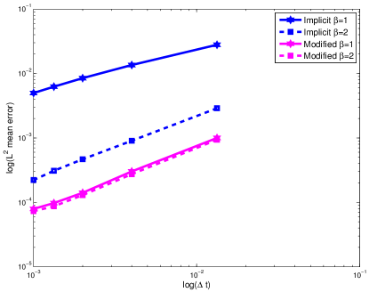
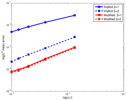
Figure 1: Convergence in the root mean square $L^{2}$ norm at $T=1$ as a function of $\Delta t$ for (40). We show convergence for noise where $\beta\in\{1,2\}$ and $\delta=0.05$ in relation (36) for finite element (a) and finite volume (b) space discretizations. We also show convergence of the standard semi–implicit scheme for the finite volume discretization. We used here 30 realizations. Note that graphs with finite element and finite volume methods give the same errors. Note that $\beta=2$ represents here the case $\beta=2-\epsilon$, with positive $\epsilon$ small enough.

Figure 2 shows convergence with exponential correlation (37). Again the new modified scheme is more accurate than the standard semi-implicit Euler–Maruyama scheme. We observe numerically a slower rate of convergence of $0.2098$ (for $b_{1}=b_{2}=0.01$) and $0.5918$ (for $b_{1}=b_{2}=0.1$) of the standard scheme compared to $0.9145$ (for $b_{1}=b_{2}=0.01$) and $0.9618$ (for $b_{1}=b_{2}=0.1$) with the modified scheme.

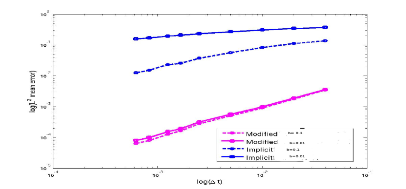
Figure 2: Convergence in the root mean square $L^{2}$ norm at $T=1$ as a function of $\Delta t$ with the noise having exponential correlation function (37) for a finite element discretisaton of (40). We used here 30 realizations and two correlation length, $b=b_{1}=b_{2}=0.1$ and $b=b_{1}=b_{2}=0.01$, $\Gamma=1$.

4.2 Stochastic advection diffusion reaction with mixed boundary conditions

For our second, and more challenging example, we consider the stochastic advection diffusion reaction SPDE (13), with $D=10^{-2}$ and mixed Neumann-Dirichlet boundary conditions on $\Omega=[0,1]\times[0,1]$. The Dirichlet boundary condition is $X=1$ at $\Gamma=\{(x,y):\;x=0\}$ and we use the homogeneous Neumann boundary conditions elsewhere.

Our goal here is to show that with the well known eigenvalues and eigenfunctions of the operator $\varDelta$ with Neumann (or Dirichlet) boundary conditions, we can apply the new scheme to mixed boundary conditions for the operator $A=D\varDelta$ without explicitly having eigenvalues and eigenfunctions of $A$. We also show that the modified scheme is more accurate than the standard semi-implicit Euler–Maruyama method.

Indeed computing the eigenfunctions and eigenvalues of $A$ with this mixed Neumann-Dirichlet boundary conditions is expensive. Let’s examine the boundary condition and put the problem in an equivalent abstract setting as (1). Using the trace operator (see EP ) in Green’s theorem yields

$$dX=(AX+F_{1}(X)+b(X))dt+dW,$$ (45)

where for $v\in H^{1}(\Omega)$

$$(Au,v)=-\int_{\Omega}D\nabla u\nabla v\,dx,$$

and

$$(bu,v)=\int_{\Gamma}\dfrac{\partial u}{\partial\nu_{A}}\gamma_{0}v\,d\sigma,\qquad\gamma_{0}v=v\mid_{\partial\Omega},\,v\in H^{1}(\Omega).$$

In this abstract setting, the linear operator is $A=D\varDelta$ but with homogeneous Neumann boundary. The explicit expression of $b$ is unknown. To deal with high Péclet flows we discretize in space using finite volumes (viewed as the finite element method (see AtThesis ; FV ). The finite volume method uses finite difference approximation of $b=\dfrac{\partial}{\partial\nu_{A}}\mid_{\Gamma}$ (see FV ; EP ). The nonlinear term is then $F=F_{1}+b$ where

$$F_{1}(u)=-\nabla\cdot(\mathbf{q}u)-\frac{u}{(u^{2}+1)},\quad u\in H^{1}(\Omega).$$ (46)

We use a heterogeneous medium with three parallel high permeability streaks, 100 times higher compared to the other part of the medium. This could represent for example a highly idealized fracture pattern. We obtain the Darcy velocity field $\mathbf{q}$ by solving (14) with Dirichlet boundary conditions on $\Gamma_{D}^{1}=\left\{0,1\right\}\times\left[0,1\right]$ and Neumann boundary conditions on $\Gamma_{N}^{1}=\left(0,1\right)\times\left\{0,1\right\}$ such that

$$p = \left\{\begin{array}[]{l}1\quad\text{in}\quad\left\{0\right\}\times\left[0,1\right]\\ 0\quad\text{in}\quad\left\{1\right\}\times\left[0,1\right]\end{array}\right.$$

and $-k\,\nabla p(\mathbf{x},t)\,\cdot\mathbf{n}=0$ in $\Gamma_{N}^{1}$. Provided $\mathbf{q}$ is bounded, since $b$ is linear, $F_{1}$ and thus $F$ satisfies Assumption 2.2 (b). We can write the semi-discrete finite volume method as

$$dX^{h}=(A_{h}X^{h}+P_{h}F_{1}(X^{h})+P_{h}b(X^{h}))+P_{h}P_{N}dW,$$ (48)

where here $A_{h}$ is the space discretization of $D\varDelta$ using only homogeneous Neumann boundary conditions and $P_{h}b(X^{h})$ comes from the approximation of diffusion flux on the Dirichlet boundary condition side (see FV ; AtThesis ). Thus we can form the noise using eigenfunctions of $\varDelta$ with full Neumann boundary conditions for the system with mixed boundary conditions. We use the noise given by (36) and compute the reference solutions using a time step of $\Delta t=1/7680$. Figure 3 shows the convergence of the modified method and the standard semi-implicit method with noise that is $H^{\beta}$ in space with $\beta\in\{1,2\}$. We observe that the temporal convergence order is close to $1/3$ for all the schemes. We observe a reduction order of convergence in Theorem 3.2. This reduction order is high, this is probably due to the velocity $\mathbf{q}$. Note that we still obtain an improvement in the accuracy over the standard semi-implicit method. Figure 3 shows the streamlines of the velocity field, computed from the elliptic equation (14). Figure 3 shows a sample reference solution with $\beta=1$ and Figure 3 shows the mean of 1000 realizations of the reference solutions also for $\beta=1$.

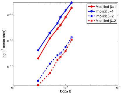
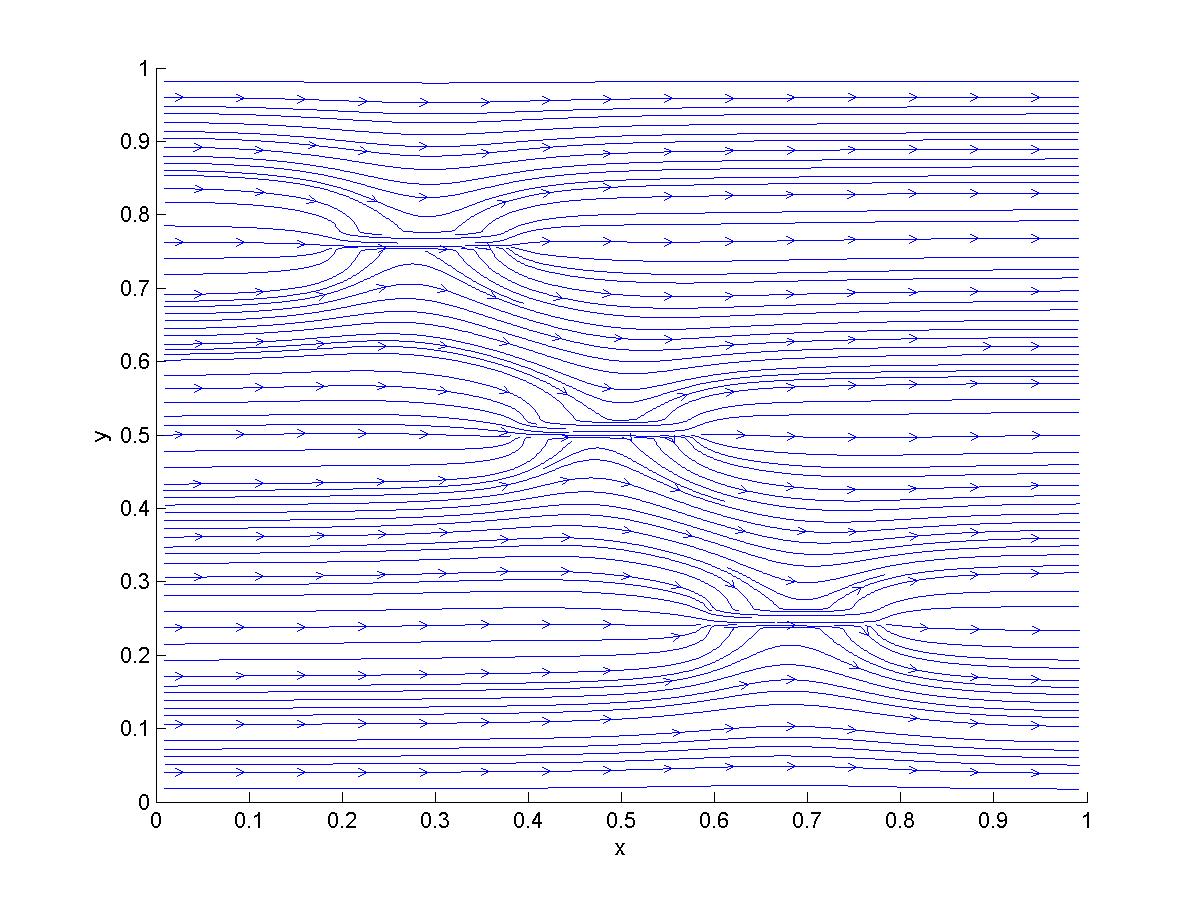
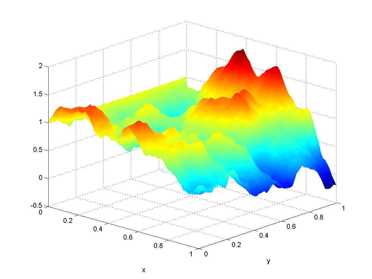
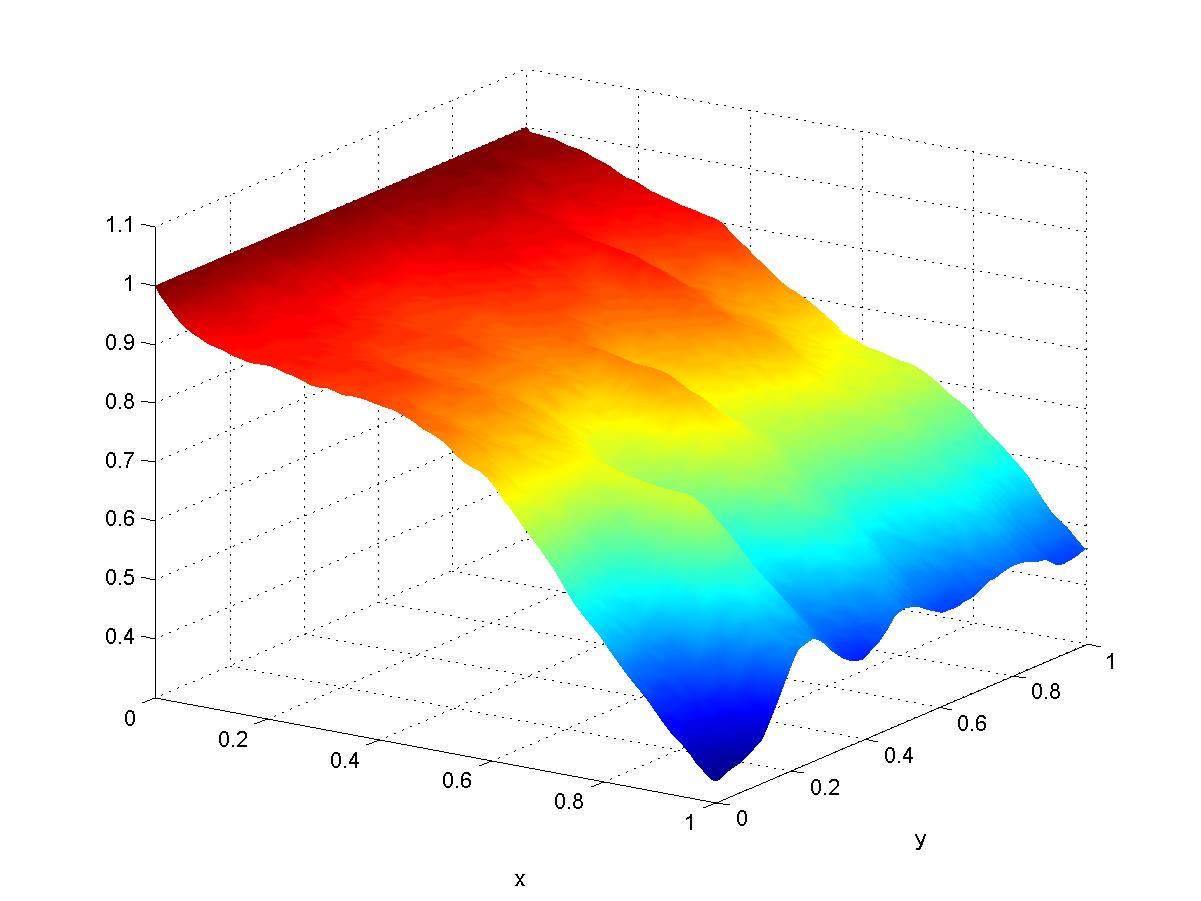
Figure 3: (a) Convergence of the root mean square $L^{2}$ norm at $T=1$ as a function of $\Delta t$ with 1000 realizations with $\Delta x=\Delta y=1/100$, $X_{0}=0$ for (1). The noise is white in time and in $H^{\beta}$ in space $\beta\in\{1,2\}$ (with $\epsilon=0.05$ in (36)). The temporal order of convergence in time is $1/3$. In (b) we plot the streamlines of the velocity field found from solving (14). In (c) we show a sample reference solution for $\beta=1$ with $\Delta t=1/7680$ while (d) displays the mean of 1000 realizations of reference solutions for $\beta=1$.

5 Proofs of the main results

5.1 Some preparatory results

We introduce the Riesz representation operator $R_{h}:V\rightarrow V_{h}$ defined by

$$(-AR_{h}v,\chi)=(-Av,\chi)=a(v,\chi)\qquad\qquad v\in V,\;\forall\chi\in V_{h}.$$ (49)

Under the regularity assumptions on the triangulation and in view of the $V-$ellipticity (16), it is well known (see lions ) that the following error bound holds for $v\in V\cap H^{r}(\Omega),$ $r\in\{1,2\}$

$$\|R_{h}v-v\|+h\|R_{h}v-v\|_{H^{1}(\Omega)}\leq Ch^{r}\|v\|_{H^{r}(\Omega)}.$$ (50)

It follows that for $v\in V\cap H^{r}(\Omega)$ $r\in\{1,2\}$

$$\|R_{h}v-v\|\leq Ch^{r}\|v\|_{H^{r}(\Omega)}.$$ (51)

Since $P_{h}$ is the $L^{2}$ orthogonal projection and $R_{h}v\in V_{h}$, we therefore have

$$\|P_{h}v-v\|=\underset{\chi\in V_{h}}{\inf}\|\chi-v\|\leq Ch^{r}\|v\|_{H^{r}(\Omega)}.$$ (52)

Since

$$\|P_{h}v-v\|\leq C\|v\|,\,v\in H,$$ (53)

We therefore have by interpolation theory

$$\|P_{h}v-v\|\leq Ch^{r}\|v\|_{r},\,v\in\mathcal{D}((-A)^{r}),\,\,0\leq r\leq 2.$$ (54)

This inequality plays a key role in our convergence proofs. A similar inequality for the interpolation operator $I_{h}$ is given in (EP, , Theorem 3.25, Theorem 3.29) or in (lions, , (2.11), pp.799). We start by examining the deterministic linear problem. Find $u\in V$ such that

$$u^{\prime}=Au\qquad\text{given}\quad u(0)=v,\quad t\in(0,T].$$ (55)

The corresponding semi–discretization in space is : find $u_{h}\in V_{h}$ such that $u_{h}^{\prime}=A_{h}u_{h}$ where $u_{h}^{0}=P_{h}v$. The full discretization of (55) using implicit Euler in time is given by

$$u_{h}^{n+1}=(\text{I}-\Delta t\;A_{h})^{-(n+1)}\;P_{h}v=S_{h,\Delta t}^{n+1}\;P_{h}v.$$ (56)

We consider the error at $t_{n}=n\Delta t$ and define the operator $T_{n}$ below

$$u(t_{n})-u_{h}^{n}=(S(t_{n})-(I-\Delta t\,A_{h})^{-n}\;P_{h})v=:T_{n}v.$$ (57)

Lemma 1

Let $0\leq\nu\leq r\leq 2$. For $v\in\mathcal{D}((-A)^{\nu/2})$, there exists a constant $C>0$ such that the following estimate holds on the numerical approximation to (55) by (56)

$$\|u(t_{n})-u_{h}^{n}\| = \|T_{n}v\|\leq Ct_{n}^{-\frac{r-\nu}{2}}(h^{r}+\Delta t^{r/2})\|v\|_{\nu}.$$ (58)

Proof

The proof can be found in (kruse, , Lemma 4.3).

Lemma 2

Let $X$ be the mild solution of (1) given in (3), such that (18) of Assumption 2.2 is satisfied for $0<\beta<2$. Let $t_{1},t_{2}\in[0,T]$, $t_{1}<t_{2}$. Assume that $X_{0}\in L_{2}(\mathbb{D},\mathcal{D}((-A)^{\beta/2}$ then we have the following.

(i) If $F$ satisfies the linear growth condition $\|F(X)\|\leq C\left(1+\|X\|\right)$, for $\sigma=\min(\beta/2,1/2)$ then

$$\mathbf{E}\|X(t_{2})-X(t_{1})\|^{2} \leq C(t_{2}-t_{1})^{2\sigma}\left(\mathbf{E}\|X_{0}\|_{\beta}^{2}+\underset{0\leq s\leq T}{\sup}\mathbf{E}\|X(s)\|^{2}+1\right).$$

(ii) If $X$ is a $H^{1}(\Omega)$-valued process and $F$ satisfies the linear growth condition

$$\|F(X)\|\leq C\left(1+\|X\|_{H^{1}(\Omega)}\right),$$ (59)

then

$$\mathbf{E}\|X(t_{2})-X(t_{1})\|^{2} \leq C(t_{2}-t_{1})^{\beta}\left(\mathbf{E}\|X_{0}\|_{\beta}^{2}+\underset{0\leq s\leq T}{\sup}\mathbf{E}\|X(s)\|_{H^{1}(\Omega)}^{2}+1\right).$$

Proof

See (xia, , (2.13) of Theorem 2.4) for the proof of part i). This proof can easily be updated for part ii) as we can bound $\|F(X(s))\|$ by (59).

5.2 Proof of Theorem 3.1

Recall that

$$X(t_{m}) = S(t_{m})X_{0}+\underset{k=0}{\sum^{m-1}}\int_{t_{k}}^{t_{k+1}}S(t_{m}-s)F(X(s))ds+\int_{0}^{t_{m}}S(t_{m}-s)dW(s)$$

$$= \overline{X}(t_{m})+O(t_{m}).$$

We now estimate $\left(\mathbf{E}\|X(t_{m})-X_{m}^{h}\|^{2}\right)^{1/2}$. By construction of the approximation from (29) and (28) we have that

$$X(t_{m})-X_{m}^{h}$$ (60)

$$= \overline{X}(t_{m})+O(t_{m})-\left(Z_{m}^{h}+P_{h}P_{N}O(t_{m})\right)$$

$$= \left(\overline{X}(t_{m})-Z_{m}^{h}\right)+\left(P_{N}(O(t_{m}))-P_{h}P_{N}(O(t_{m}))\right)+\left(O(t_{m})-P_{N}(O(t_{m}))\right)$$

$$= I+II+III,$$

and $Z_{m}^{h}$ is given by (28). Then

$$\left(\mathbf{E}\|X(t_{m})-X_{m}^{h}\|^{2}\right)^{1/2}\leq\left(\mathbf{E}\|I\|^{2}\right)^{1/2}+\left(\mathbf{E}\|II\|^{2}\right)^{1/2}+\left(\textbf{E}\|III\|^{2}\right)^{1/2}$$

and we estimate each term. Since the first term will require the most work we estimate $II$ and $III$ first. Let us examine $\left(\mathbf{E}\|II\|^{2}\right)^{1/2}$. To do this we use the finite element estimate (54), the regularity of the noise and the fact that $P_{N}$ is bounded. Then for $0\leq\beta\leq 2$ , if $O(t_{m})\in\mathcal{D}((-A)^{\frac{\beta}{2}})$ we have

$$\mathbf{E}\|II\|^{2}\leq Ch^{2\beta}\mathbf{E}\|P_{N}(O(t_{m}))\|_{\beta}^{2}\leq Ch^{2\beta}\mathbf{E}\|O(t_{m})\|_{\beta}^{2}.$$

Using the Ito isometry, (xia, , Lemma 3.2) and (18) of Assumption 2.2 yields

$$\mathbf{E}\|II\|^{2} \leq Ch^{2\beta}\int_{0}^{t_{m}}\|(-A)^{\beta/2}S(t_{m}-s)Q^{1/2}\|_{\mathcal{L}_{2}(H)}^{2}ds$$

$$\leq Ch^{2\beta}\|(-A)^{(\beta-1)/2}Q^{1/2}\|_{\mathcal{L}_{2}(H)}^{2}.$$

For the third term $III$ we have

$$\mathbf{E}\|III\|^{2} = \mathbf{E}\|(\text{I}-P_{N})O(t_{m})\|^{2}$$

$$= \mathbf{E}\|(\text{I}-P_{N})(-A)^{-\beta/2}(-A)^{\beta/2}O(t_{m})\|^{2},$$

and so using again (xia, , Lemma 3.2), (18) of Assumption 2.2

$$\mathbf{E}\|III\|^{2} \leq \|(\text{I}-P_{N})(-A)^{-\beta/2}\|_{L(L^{2}(\Omega))}^{2}\mathbf{E}\|(-A)^{\beta/2}O(t_{m})\|^{2}$$

$$\leq \|(-A)^{(\beta-1)/2}Q^{1/2}\|_{\mathcal{L}_{2}(H)}^{2}\left(\underset{j\in\mathbb{N}^{d}\backslash\mathcal{I}_{N}}{\inf}\lambda_{j}\right)^{-\beta}$$

$$\leq C\left(\underset{j\in\mathbb{N}^{d}\backslash\mathcal{I}_{N}}{\inf}\lambda_{j}\right)^{-\beta}.$$

To estimate $I$, we follow the approach in xia

$$I = S(t_{m})X_{0}-S_{h,\Delta t}^{(m)}P_{h}X_{0}$$

$$+ \underset{k=0}{\sum^{m-1}}\int_{t_{k}}^{t_{k+1}}S(t_{m}-s)F(X(s))ds-\underset{k=0}{\sum^{m-1}}\left(\int_{t_{k}}^{t_{k+1}}S_{h,\Delta t}^{(m-k)}P_{h}F(X_{k}^{h})ds\right)$$

$$= I_{1}+I_{2},$$

then

$$\mathbf{E}\|I\|^{2}\leq 2\left(\mathbf{E}\|I_{1}\|^{2}+\mathbf{E}\|I_{2}\|^{2}\right).$$

According to Lemma 1, for $X_{0}\in L_{2}\left(\mathbb{D},\mathcal{D}((-A)^{\beta/2})\right),\,0<\beta<2$ we have

$$\left(\mathbf{E}\|I_{1}\|^{2}\right)^{1/2}\leq C(h^{\beta}+\Delta t^{\beta/2}).$$ (61)

To estimate $\mathbf{E}\|I_{2}\|^{2}$ we have

$$I_{2} = \underset{k=0}{\sum^{m-1}}\int_{t_{k}}^{t_{k+1}}\left(S(t_{m}-t_{k})-S_{h,\Delta t}^{(m-k)}P_{h}\right)F(X(s))ds$$

$$+\underset{k=0}{\sum^{m-1}}\int_{t_{k}}^{t_{k+1}}\left(S(t_{m}-s)-S(t_{m}-t_{k})\right)F(X(s))ds$$

$$+\underset{k=0}{\sum^{m-1}}\int_{t_{k}}^{t_{k+1}}S_{h,\Delta t}^{(m-k)}P_{h}\left(F(X(s)-F(X(t_{k}))\right)ds$$

$$+\underset{k=0}{\sum^{m-1}}\int_{t_{k}}^{t_{k+1}}S_{h,\Delta t}^{(m-k)}P_{h}\left(F(X(t_{k}))-F(X_{k}^{h})\right)ds$$

$$= I_{2}^{1}+I_{2}^{2}+I_{2}^{3}+I_{2}^{4}.$$

Using again Lemma 1, for $0<\beta<2$ we have

$$\left(\mathbf{E}\|I_{2}^{1}\|^{2}\right)^{1/2}$$

$$\leq \underset{k=0}{\sum^{m-1}}\int_{t_{k}}^{t_{k+1}}\left(\mathbf{E}\|\left(S(t_{m}-t_{k})-S_{h,\Delta t}^{(m-k)}P_{h}\right)F(X(s))\|^{2}\right)^{1/2}ds$$

$$\leq C(h^{(\beta)}+\Delta t^{\beta/2}\left(\underset{k=0}{\sum^{m-1}}\int_{t_{k}}^{t_{k+1}}(t_{m}-t_{k})^{-\beta/2}ds\right)^{1/2}\left(1+\underset{0\leq s\leq T}{\sup}\mathbf{E}\|(X(s))\|^{2}\right)^{1/2}$$

$$\leq C(h^{\beta}+\Delta t^{\beta/2})\left(\int_{0}^{t_{m}}(t_{m}-t_{k})^{-\beta/2}ds\right)^{1/2}$$

$$\leq C(h^{\beta}+\Delta t^{\beta/2}).$$

Let us estimate $\left(\mathbf{E}\|I_{2}^{2}\|^{2}\right)^{1/2}$. By Proposition 1, for $0\leq t_{1}<t_{2}\leq T$ we have

$$\|S(t_{2})-S(t_{1})\|_{L(L^{2}(\Omega))} = \|(-A)S(t_{1})(-A)^{-1}\left(\mathbf{I}-S(t_{2}-t_{1})\right)\|_{L(L^{2}(\Omega))}$$

$$\leq \dfrac{(t_{2}-t_{1})}{t_{1}}.$$

Splitting the estimation and using (5.2) in the second part yields

$$\left(\mathbf{E}\|I_{2}^{2}\|^{2}\right)^{1/2} \leq \left(\underset{k=0}{\sum^{m-1}}\int_{t_{k}}^{t_{k+1}}\|S(t_{m}-s)-S(t_{m}-t_{k})\|_{L(L^{2}(\Omega))}ds\right)$$

$$\times\left(\underset{0\leq s\leq T}{\sup}\mathbf{E}\|F(X(s))\|^{2}\right)^{1/2}$$

$$\leq C\left(\int_{t_{m-1}}^{t_{m}}\|S(t_{m}-s)-S(t_{m}-t_{m-1})\|_{L(L^{2}(\Omega))}ds\right.$$

$$\left.+\underset{k=0}{\sum^{m-2}}\int_{t_{k}}^{t_{k+1}}\left(\dfrac{s-t_{k}}{t_{m}-s}\right)ds\right).$$

Using the fact that the operator $S(t)$ is bounded yields

$$\int_{t_{m-1}}^{t_{m}}\|S(t_{m}-s)-S(t_{m}-t_{m-1})\|_{L(L^{2}(\Omega))}ds\leq C\Delta t,$$

and then

$$\left(\mathbf{E}\|I_{2}^{2}\|^{2}\right)^{1/2} \leq C\left(\Delta t+\underset{k=0}{\sum^{m-2}}\left((m-k-1)\Delta t\right)^{-1}\int_{t_{k}}^{t_{k+1}}\left(s-t_{k}\right)ds\right)$$

$$\leq C\left(\Delta t+\Delta t\underset{k=0}{\sum^{m-2}}\left(m-k-1\right)^{-1}\right).$$

Noting that the sum above is bounded by $\ln(M)$ we have

$$\left(\textbf{E}\|I_{2}^{2}\|^{2}\right)^{1/2} \leq C(\Delta t+\Delta t|\ln(\Delta t)|).$$

The estimation of $\mathbf{E}\|I_{2}^{3}\|^{2}$ follows the one in xia using Lemma 2. We provide some keys steps, the main difference comes from the different space discretization. By Taylor expansion

$$(X(s)-F(X(t_{k}))$$

$$= F^{\prime}(X(t_{k}))(X(s)-X(t_{k}))+RF$$

$$= F^{\prime}(X(t_{k}))\left((S(s-t_{k})-I)X(t_{k})+\int_{t_{k}}^{s}(S(s-\tau)F(X(\tau))d\tau+\int_{t_{k}}^{s}(S(s-\tau)dW(\tau)\right)$$

where $RF=\int_{0}^{1}F^{\prime\prime}(X(t_{k}))+r(X(s)-X(t_{k}))(X(s)-X(t_{k}),X(s)-X(t_{k}))dr$. Then,

$$\left(\mathbf{E}\|I_{2}^{3}\|^{2}\right)^{1/2}$$

$$= \left(\mathbf{E}\Big{\|}\underset{k=0}{\sum^{m-1}}\int_{t_{k}}^{t_{k+1}}S_{h,\Delta t}^{(m-k)}P_{h}F^{\prime}(X(t_{k}))\left((S(s-t_{k})-I)X(t_{k})\right)ds\Big{\|}^{2}\right)^{1/2}$$

$$+ \left(\mathbf{E}\Big{\|}\underset{k=0}{\sum^{m-1}}\int_{t_{k}}^{t_{k+1}}S_{h,\Delta t}^{(m-k)}P_{h}F^{\prime}(X(t_{k}))\int_{t_{k}}^{s}(S(s-\tau)F(X(\tau))d\tau ds\Big{\|}^{2}\right)^{1/2}$$

$$+ \left(\mathbf{E}\Big{\|}\underset{k=0}{\sum^{m-1}}\int_{t_{k}}^{t_{k+1}}S_{h,\Delta t}^{(m-k)}P_{h}F^{\prime}(X(t_{k}))\int_{t_{k}}^{s}(S(s-\tau)dW(\tau)ds\Big{\|}^{2}\right)^{1/2}$$

$$+ \left(\mathbf{E}\Big{\|}\underset{k=0}{\sum^{m-1}}\int_{t_{k}}^{t_{k+1}}S_{h,\Delta t}^{(m-k)}P_{h}RFds\Big{\|}^{2}\right)^{1/2}$$

$$= I_{21}^{3}+I_{22}^{3}+I_{23}^{3}+I_{24}^{3}.$$

Let us estimate $I_{21}^{3}$. Assumption 2.2 yields

$$I_{21}^{3}$$

$$\leq \underset{k=0}{\sum^{m-1}}\int_{t_{k}}^{t_{k+1}}\left(\mathbf{E}\Big{\|}S_{h,\Delta t}^{(m-k)}P_{h}F^{\prime}(X(t_{k}))\left((S(s-t_{k})-I)X(t_{k})\right)\Big{\|}^{2}\right)^{1/2}ds$$

$$\leq \underset{k=0}{\sum^{m-1}}\int_{t_{k}}^{t_{k+1}}\|S_{h,\Delta t}^{(m-k)}(-A_{h})^{\delta/2}\|_{L(L^{2}(\Omega))}$$

$$\times\left(\mathbf{E}\Big{\|}(-A_{h})^{-\delta/2}P_{h}F^{\prime}(X(t_{k}))\left((S(s-t_{k})-I)X(t_{k})\right)\Big{\|}^{2}\right)^{1/2}ds$$

The operator $S_{h,\Delta t}$ satisfies the smoothing properties analogous to $S(t)$ independently of $h$ (see for example Stig ; ElliottLarsson ), we find for $t_{m}=m\Delta t>0$

$$S_{h,\Delta t}^{m}(-A_{h})^{\delta/2}\leq Ct_{m}^{-\delta/2}.$$

Note that for $u\in H=L^{2}(\Omega)$

$$\|(-A_{h})^{-\frac{\delta}{2}}P_{h}u\|=\underset{v_{h}\in V_{h}}{\sup}\dfrac{((-A_{h})^{-\delta/2}P_{h}u,v_{h})}{\|v_{h}\|}=\underset{v_{h}\in V_{h}}{\sup}\dfrac{(P_{h}u,(-A_{h}^{*})^{-\delta/2}v_{h})}{\|v_{h}\|}.$$ (62)

Using the definition of $P_{h}$ we have

$$\|(-A_{h})^{-\frac{\delta}{2}}P_{h}u\| = \underset{v_{h}\in V_{h}}{\sup}\dfrac{(u,(-A_{h}^{*})^{-\delta/2}v_{h})}{\|v_{h}\|}=\underset{w_{h}\in V_{h}}{\sup}\dfrac{(u,w_{h})}{\|(-A_{h}^{*})^{\delta/2}v_{h}\|}$$ (63)

$$\leq C\underset{w_{h}\in V_{h}}{\sup}\dfrac{(u,w_{h})}{\|v_{h}\|_{\delta}}=\|u\|_{-\delta}=\|(-A)^{-\delta/2}u\|.$$

Using (63) and (5.2) yields

$$I_{21}^{3} \leq C\underset{k=0}{\sum^{m-1}}\int_{t_{k}}^{t_{k+1}}(t_{m}-t_{k})^{-\delta/2}\left(\mathbf{E}\Big{\|}(-A)^{-\delta/2}F^{\prime}(X(t_{k}))\left((S(s-t_{k})-I)X(t_{k})\right)\Big{\|}^{2}\right)^{1/2}ds$$

The rest of the estimation follows (xia, , $I_{31}$) using Lemma 2, and we have

$$I_{21}^{3}\leq C(\Delta t^{\min(\beta,1)}).$$

It is obvious that $I_{22}^{3}\leq C\Delta t.$ The estimation of $I_{23}^{3}$ follows from (xia, , $I_{33}$) by replacing $P_{N}$ by $P_{h}$ and $E(t_{m}-s)$ by $S_{h,\Delta t}^{(m-k)}$ to get $I_{23}^{3}\leq C\Delta t^{\min(1+\beta,2)}.$ The estimation of $I_{24}^{3}$ follows from (xia, , $I_{34}$) by replacing $P_{N}$ by $P_{h}$ and $E(t_{m}-s)$ by $S_{h,\Delta t}^{(m-k)}$ and we finally have $I_{24}^{3}\leq\Delta t^{\min(\beta,1)}.$
Putting the estimates on $I_{21}^{3}$, $I_{22}^{3}$, $I_{23}^{3}$ and $I_{24}^{3}$ together we see that

$$\left(\ \mathbf{E}\|I_{2}^{2}\|^{2}\right)^{1/2}\leq C\Delta t^{\min(\beta,1)}.$$ (64)

For $\mathbf{E}\|I_{2}^{3}\|^{2}$, we obviously have

$$\left(\mathbf{E}\|I_{2}^{3}\|^{2}\right)^{1/2}\leq C\underset{k=0}{\sum^{m-1}}\int_{t_{k}}^{t_{k+1}}\left(\mathbf{E}\|X(t_{k})-X_{k}^{h}\|^{2}\right)^{1/2}ds.$$ (65)

Combining the estimates of $\mathbf{E}\|I\|^{2}$ and $\mathbf{E}\|II\|^{2}$ and applying the discrete Gronwall lemma completes the proof.

5.3 Proof of Theorem 3.2

The estimation of $I$ and $II$ is the same as before. We now estimate the term $I$ from (60) when there is non-zero advection. As above we have

$$I = T_{m}X_{0}+\underset{k=0}{\sum^{m-1}}\int_{t_{k}}^{t_{k+1}}S(t_{m}-s)F(X(s))-S_{h,\Delta t}^{(m-k)}P_{h}F(Z_{k}^{h}+P_{h}P_{N}O(t_{k}))ds$$ (66)

$$= T_{m}X_{0}+\underset{k=0}{\sum^{m-1}}\int_{t_{k}}^{t_{k+1}}S_{h,\Delta t}^{(m-k)}P_{h}(F(X(t_{k}))-F(Z_{k}^{h}+P_{h}P_{N}O(t_{k}))))ds$$

$$+\underset{k=0}{\sum^{m-1}}\int_{t_{k}}^{t_{k+1}}S_{h,\Delta t}^{(m-k)}P_{h}(F(X(s))-F(X(t_{k})))ds$$

$$+\underset{k=0}{\sum^{m-1}}\int_{t_{k}}^{t_{k+1}}(S(t_{m}-t_{k})-S_{h,\Delta t}^{(m-k)}P_{h})F(X(s))ds$$

$$+\underset{k=0}{\sum^{m-1}}\int_{t_{k}}^{t_{k+1}}(S(t_{m}-s)-S(t_{m}-t_{k}))F(X(s))ds$$

$$= I_{1}+I_{2}+I_{3}+I_{4}+I_{5}.$$

The estimation of $I_{1}$ is the same as for Theorem 3.1. If $F$ satisfies Assumption 2.2(b), using (63) with $\delta=1$ yields

$$(\mathbf{E}\|I_{2}\|^{2})^{1/2}$$

$$\leq \underset{k=0}{\sum^{m-1}}\int_{t_{k}}^{t_{k+1}}\left(\mathbf{E}\|S_{h,\Delta t}^{(m-k)}P_{h}\left(F(X(t_{k}))-F(Z_{k}^{h}+P_{h}P_{N}O(t_{k}))\right)\|^{2}\right)^{1/2}ds$$

$$= \underset{k=0}{\sum^{m-1}}\int_{t_{k}}^{t_{k+1}}\left(\mathbf{E}\|S_{h,\Delta t}^{(m-k)}(-A_{h})^{1/2}(-A_{h})^{-1/2}P_{h}\left(F(X(t_{k}))-F(Z_{k}^{h}+P_{h}P_{N}O(t_{k}))\right)\|^{2}\right)^{1/2}ds$$

$$\leq C\underset{k=0}{\sum^{m-1}}\int_{t_{k}}^{t_{k+1}}(t_{m}-t_{k})^{-1/2}\left(\mathbf{E}\|F(X(t_{k}))-F(Z_{k}^{h}+P_{h}P_{N}O(t_{k}))\|_{-1}^{2}\right)^{1/2}ds$$

$$\leq C\underset{k=0}{\sum^{m-1}}\int_{t_{k}}^{t_{k+1}}(t_{m}-t_{k})^{-1/2}\left(\mathbf{E}\|X(t_{k})-X_{k}^{h}\|^{2}\right)^{1/2}ds.$$

Let us estimate $(\mathbf{E}\|I_{3}\|^{2})^{1/2}$. Once again using the Lipschitz condition and smoothing property of $S_{h,\Delta t}$

$$(\mathbf{E}\|I_{3}\|^{2})^{1/2} \leq C\underset{k=0}{\sum^{m-1}}\int_{t_{k}}^{t_{k+1}}(t_{m}-t_{k})^{-1/2}\left(\mathbf{E}\|F(X(s))-F(X(t_{k}))\|_{-1}\right)^{1/2}ds$$

$$\leq C\underset{k=0}{\sum^{m-1}}\int_{t_{k}}^{t_{k+1}}(t_{m}-t_{k})^{-1/2}(\mathbf{E}\|X(s)-X(t_{k})\|^{2})^{1/2}ds$$

Since

$$\underset{k=0}{\sum^{m-1}}\int_{t_{k}}^{t_{k+1}}(t_{m}-t_{k})^{-1/2}ds\leq 2\sqrt{T}.$$

Then if $X_{0}\in L_{2}(\mathbb{D},\mathcal{D}((-A)^{\beta/2})),\,0<\beta<2$ such that $X(t)$ is a $H^{1}(\Omega)$- valued process

$$(\mathbf{E}\|I_{3}\|^{2})^{1/2}\leq C(\Delta t)^{\min(\beta/2,1/2)}\left(\mathbf{E}\|X_{0}\|_{\beta}^{2}+\underset{0\leq s\leq T}{\sup}\mathbf{E}\|X(s)\|_{H^{1}(\Omega)}^{2}+1\right)^{1/2},$$

From Lemma 1, for $0\leq\beta<2$ such that $X(t)$ is a $H^{1}(\Omega)$- valued process, we have

$$(\mathbf{E}\|I_{4}\|^{2})^{1/2} \leq \underset{k=0}{\sum^{m-1}}\int_{t_{k}}^{t_{k+1}}\left(\mathbf{E}\|T_{m}(t_{m}-t_{k})F(X(s))\|^{2}\right)^{1/2}ds$$

$$\leq C(h^{\beta}+\Delta t^{\beta/2})\left(\underset{k=0}{\sum^{m-1}}\int_{t_{k}}^{t_{k+1}}(t_{m}-t_{k})^{-\beta/2}ds\right)\left(\underset{0\leq s\leq T}{\sup}\mathbf{E}\|F(X(s))\|^{2}\right)^{1/2}$$

$$\leq C(h^{\beta}+\Delta t^{\beta/2})\left(1+\left(\underset{0\leq s\leq T}{\sup}\mathbf{E}\|X(s)\|_{H^{1}(\Omega)}^{2}\right)^{1/2}\right)$$

$$\leq C(h^{\beta}+\Delta t^{\beta/2})$$

As in the estimation of $I_{2}^{2}$ in the previous section, if $X(t)$ is a $H^{1}(\Omega)$- valued process we have

$$(\mathbf{E}\|I_{5}\|^{2})^{1/2} \leq C(\Delta t+\Delta t|\ln(\Delta t)|).$$

Combining our estimates $\left(\mathbf{E}\|I\|^{2}\right)^{1/2},\left(\mathbf{E}\|II\|^{2}\right)^{1/2}$ and $\left(\mathbf{E}\|III\|^{2}\right)^{1/2}$ and using the discrete Gronwall lemma concludes the proof.

5.4 Proof of Proposition 2

Let $b$ and $\lambda$ be two real numbers, then the following result holds

$$\int_{-\infty}^{+\infty}\exp\left(-\dfrac{\pi}{4}\left(\frac{x^{2}}{b^{2}}\right)\right)\cos(\lambda x)dx=2b\exp\left[-\dfrac{1}{\pi}\left(\lambda b\right)^{2}\right].$$ (67)

Recall DaPZ that the covariance operator $Q$ may be defined for $f\in L^{2}(\Omega)$ by

$$Qf(x)=\int_{\Omega}C_{r}(x,y)f(y)dy.$$

Indeed we have

$$4b_{1}b_{2}\int_{0}^{L_{1}}\int_{0}^{L_{2}}C_{r}((x_{1},y_{1});(x_{2},y_{2}))\cos(\lambda_{i}^{(1)}x_{2})\cos(\lambda_{j}^{(2)}y_{2})dy_{2}dx_{2}$$

$$= \Gamma\;\int_{0}^{L_{1}}\exp\left(-\dfrac{\pi}{4}\left(\dfrac{\left(x_{2}-x_{1}\right)^{2}}{b_{1}^{2}}\right)\right)\cos(\lambda_{i}^{(1)}x_{2})dx_{2}$$

$$\times\int_{0}^{L_{2}}\exp\left(-\dfrac{\pi}{4}\left[\dfrac{\left(y_{2}-y_{1}\right)^{2}}{b_{2}^{2}}\right]\right)\cos(\lambda_{j}^{(2)}y_{2})dy_{2}$$

$$= \Gamma\;\int_{-x_{1}}^{L_{1}-x_{1}}\exp\left(-\dfrac{\pi}{4}\left(\dfrac{x^{2}}{b_{1}^{2}}\right)\right)\cos(\lambda_{i}^{(1)}(x+x_{1}))dx$$

$$\times\int_{-y_{1}}^{L_{2}-y_{1}}\exp\left(-\dfrac{\pi}{4}\left(\dfrac{x^{2}}{b_{2}^{2}}\right)\right)\cos(\lambda_{j}^{(2)}(x+y_{1})dx).$$

For $b_{i}\ll L_{i}$, because of the strong decay, we approximate the integral in the finite domain by the integral in infinite domain where we can evaluate exactly

$$4b_{1}b_{2}\int_{0}^{L_{1}}\int_{0}^{L_{2}}C_{r}((x_{1},y_{1});(x_{2},y_{2}))\cos(\lambda_{i}^{(1)}x_{2})\cos(\lambda_{j}^{(2)}y_{2})dy_{2}dx_{2}$$

$$\approx \Gamma\;\int_{-\infty}^{+\infty}\exp\left(-\dfrac{\pi}{4}\left(\dfrac{x^{2}}{b_{1}^{2}}\right)\right)\cos(\lambda_{i}^{(1)}(x+x_{1}))dx$$

$$\times\int_{-\infty}^{+\infty}\exp\left(-\dfrac{\pi}{4}\left(\dfrac{x^{2}}{b_{2}^{2}}\right)\right)\cos(\lambda_{j}^{(2)}(x+y_{1}))dx$$

$$= 4b_{1}b_{2}\cos(\lambda_{i}^{(1)}\,x_{1})\cos(\lambda_{j}^{(2)}\,y_{1})\,\Gamma\,\exp\left(-\dfrac{1}{\pi}\left((\lambda_{i}^{(1)}b_{1})^{2}+(\lambda_{j}^{(2)}b_{2})^{2}\right)\right).$$

It is important to notice that we have used the fact that

$$\int_{-\infty}^{+\infty}\exp\left(-\dfrac{\pi}{4}\left(\dfrac{x^{2}}{b_{i}^{2}}\right)\right)\cos(\lambda_{j}^{(i)}x)dx = 2b_{i}\exp\left[-\dfrac{1}{\pi}\left((\lambda_{j}^{(i)}b_{i})^{2}\right)\right]\;\;\;\;i\in\left\{1,2\right\}$$

by (67) and

$$\int_{-\infty}^{+\infty}\exp\left(-\dfrac{\pi}{4}\left(\dfrac{x^{2}}{b_{i}^{2}}\right)\right)\sin(\lambda_{j}^{(i)}x)dx = 0$$

because the integrand is an odd function. Then the corresponding values of $\left\{q_{i,j}\right\}_{i+j>0}$ in the representation (2) is given by

$$q_{i,j}=\Gamma\exp\left[-\dfrac{1}{2\pi}\left((\lambda_{i}^{(1)}b_{1})^{2}+(\lambda_{j}^{(2)}b_{2})^{2}\right)\right].$$

Acknowledgements

We would like to thank Dr A. Jentzen for very useful discussions at an early stage of this paper. These were made possible through an arc–daad grant number 1333. Antoine Tambue was also funded by the Overseas Research Students Awards Scheme (ORSAS), Heriot Watt University and Robert Bosch Stiftung through the AIMS ARETE chair programme.

References

- (1) Allen, E.J., Novosel, S.J., Zhang, Z.: Finite element and difference approximation of some linear stochastic partial differential equations. Stochastics Stochastics Rep. 64(1-2), 117–142 (1998)
- (2) Bear, J.: Dynamics of Fluids in Porous Media. Dover (1988)
- (3) Bedient, P., Rifai, H., Newell, C.: Ground Water Contamination: Transport and Remediation. Prentice Hall PTR , Englewood Cliffs, New Jersey 07632 (1994)
- (4) Chow, P.L.: Stochastic Partial Differential Equations. Applied Mathematics and nonlinear Science. Chapman & Hall / CRC (2007). ISBN-1-58488-443-6
- (5) Da Prato, G., Zabczyk, J.: Stochastic Equations in Infinite Dimensions, Encyclopedia of Mathematics and its Applications, vol. 44. Cambridge University Press, Cambridge (1992)
- (6) Elliott, C.M., Larsson, S.: Error estimates with smooth and nonsmooth data for a finite element method for the Cahn-Hilliard equation. Math. Comp. 58, 603–630 (1992)
- (7) Eymard, R., Gallouet, T., Herbin, R.: Finite volume methods. In: P.G. Ciarlet, J.L. Lions (eds.) Handbook of Numerical Analysis, vol. 7, pp. 713–1020. North-Holland (2003)
- (8) Fujita, H., Suzuki, T.: Evolutions problems (part1). In: P.G. Ciarlet, J.L. Lions (eds.) Handbook of Numerical Analysis, vol. II, pp. 789–928. North-Holland (1991)
- (9) Hausenblas, E.: Approximation for semilinear stochastic evolution equations. Potential Analysis 18(2):141–186 (2003)
- (10) Henry, D.: Geometric theory of semilinear parabolic equations. No. 840 in Lecture notes in mathematics. Springer (1981)
- (11) Jentzen, A.: Pathwise numerical approximations of SPDEs. Potential Analysis 31(4):375–404 (2009)
- (12) Jentzen, A.: Higher order pathwise numerical approximations of SPDES with additive noise. SIAM J. Num. Anal. 49(2), 642–667 (2011)
- (13) Jentzen, A., Kloeden, P.E.: Overcoming the order barrier in the numerical approximation of SPDEs with additive space-time noise. Proc. R. Soc. A 465(2102):649–667 (2009)
- (14) Jentzen, A., Kloeden, P.E., Winkel, G.: Efficient simulation of nonlinear parabolic SPDES with additive noise. Annals of Applied Probability 21(3):908–950 (2011)
- (15) Katsoulakis, M.A., Kossioris, G., Lakkis, O.: Noise regularization and computations for the 1-dimensional stochastic Allen–Cahn problem. Interfaces and Free Boundaries 9(1), 1–30 (2007). DOI: 10.4171/IFB/154
- (16) Knabner, P., Angermann, L.: Numerical methods for elliptic and parabolic partial differential equations solution. Springer (2000)
- (17) Kossioris, G.T., Zouraris, G.E.: Fully-discrete finite element approximations for a fourth-order linear stochastic parabolic equation with additive space-time white noise. ESAIM p. 289 (2010). DOI: 10.1051/m2an/2010003
- (18) Kovács, M., Larsson, S., Lindgren, F.: Strong convergence of the finite element method with truncated noise for semilinear parabolic stochastic equations with additive noise. Numer.Algor. 53, 309–320 (2010)
- (19) Kovács, M., Lindgren, F., Larsson, S.: Spatial approximation of stochastic convolutions. J. Comput. Appl. Math. 235, 3554–3570 (2011)
- (20) Larsson, S.: Nonsmooth data error estimates with applications to the study of the long-time behavior of finite element solutions of semilinear parabolic problems (1992). Preprint 1992-36, Department of Mathematics, Chalmers University of Technology
- (21) Larsson, S.: Semilinear parabolic partial differential equations — theory, approximation and application. In: G. Ekhaguere, C.K. Ayo, M.B. Olorunsaiye (eds.) New Trends in the Mathematical and Computer Sciences, vol. 3, pp. 153–194 (2006). ISBN: 978–37246–2–2
- (22) G. J. Lord, C. E. Powell and T. Shardlow An Introduction to Computational Stochastic PDEs CUP, 2014
- (23) Lord, G., Tambue, A.: Stochastic exponential integrators for finite element discretization of SPDE for multiplicative and additive noise. IMA Journal of Numerical Analysis (2012), doi:10.1093/imanum/drr059 (2012)
- (24) Lord, G.J., Tambue, A.: Stochastic exponential integrators for finite element discretization of SPDEs with additive noise (2010). Http://arxiv.org/abs/1005.5315,
- (25) R. Kruse. Optimal error estimates of galerkin finite element methods for stochastic partial differential equations with multiplicative noise. IMA Journal of Numerical Analysis, 34(1)(2014) 217–251.
- (26) Prévôt, C., Röckner, M.: A Concise Course on Stochastic Partial Differential Equations. Springer (2007). ISBN-10: 3540707808
- (27) Shardlow, T.: Numerical simulation of stochastic PDEs for excitable media. J. Comput. Appl. Math. 175(2), 429–446 (2005).
- (28) Tambue, A.: Efficient numerical methods for porous media flow. Ph.D. thesis, Department of Mathematics, Heriot–Watt University (2010)
- (29) Thomée, V.: Galerkin finite element methods for parabolic problems. Springer Series in Computational Mathematics (1997)
- (30) Xiaojie Wang, and Ruisheng Qi. A note on an accelerated exponential Euler method for parabolic SPDEs with additive noise. Applied Mathematics Letters 46 (2015) 31–37.
- (31) Yan, Y.: Semidiscrete Galerkin approximation for a linear stochastic parabolic partial differential equation driven by an additive noise. BIT Numerical Mathematics 44(4), 829–847 (2004). DOI:10.1007/s10543-004-3755-5
- (32) Yan, Y.: Galerkin finite element methods for stochastic parabolic partial differential equations. SIAM J. Num. Anal. 43(4), 1363–1384 (2005)