A fast solver for linear systems
with displacement structure

Abstract

We describe a fast solver for linear systems with reconstructable Cauchy-like structure, which requires $O(rn^{2})$ floating point operations and $O(rn)$ memory locations, where $n$ is the size of the matrix and $r$ its displacement rank. The solver is based on the application of the generalized Schur algorithm to a suitable augmented matrix, under some assumptions on the knots of the Cauchy-like matrix. It includes various pivoting strategies, already discussed in the literature, and a new algorithm, which only requires reconstructability. We have developed a software package, written in Matlab and C-MEX, which provides a robust implementation of the above method. Our package also includes solvers for Toeplitz(+Hankel)-like and Vandermonde-like linear systems, as these structures can be reduced to Cauchy-like by fast and stable transforms. Numerical experiments demonstrate the effectiveness of the software.

Keywords: displacement structure, Cauchy-like, Toeplitz(+Hankel)-like, Vandermonde-like, generalized Schur algorithm, augmented matrix, Matlab toolbox.

1 Introduction

The idea to connect the solution of some linear problems to suitable augmented matrices has often been used in linear algebra; see, e.g., [4, 6, 26] for an application to full rank least squares problems. More recently, it was proposed [17] to solve various computational problems involving Toeplitz matrices by evaluating a Schur complement of a suitable augmented matrix.

The reason for this approach lies in the fact that Toeplitz matrices, as well as other classes of structured matrices, can be expressed as the solution of a displacement equation [9, 18], and that this property is inherited by their Schur complements of any order. This fact allows one to store a structured matrix of dimension $n$ in $O(n)$ memory locations and, which is most important, to apply a fast implementation of the Gauss triangularization method (the generalized Schur algorithm) operating directly on the displacement information associated to the matrix [10, 13, 15]; see also [19, 20] for a review.

In this paper we use the mathematical tools above mentioned to devise a fast algorithm to solve the linear system

$$C\mathbf{x}=\mathbf{b},$$ (1)

where $\mathbf{b}\in{\mathbb{C}}^{n}$ and $C\in{\mathbb{C}}^{n\times n}$ is a Cauchy-like matrix; this means that

$$C_{ij}=\dfrac{\boldsymbol{\phi}_{i}^{*}\,\boldsymbol{\psi}_{j}}{t_{i}-s_{j}},$$ (2)

where $\boldsymbol{\phi}_{i},\boldsymbol{\psi}_{j}\in{\mathbb{C}}^{r}$, $t_{i},s_{j}\in{\mathbb{C}}$, $i,j=1,\dots,n$, and the asterisk denotes the conjugate transpose.

Given a matrix

$$M=\begin{bmatrix}A&B\\ C&D\end{bmatrix},$$

with $A\in{\mathbb{C}}^{n\times n}$ invertible, we denote its Schur complement of order $n$ by

$${\mathcal{S}}_{n}(M)=D-CA^{-1}B.$$

We associate to the system (1) the augmented matrix

$$\mathcal{A}_{C,\mathbf{b}}=\begin{bmatrix}C&\mathbf{b}\\ -I_{n}&O\end{bmatrix},$$ (3)

where $I_{n}$ is the identity matrix of size $n$ and $O$ is a null matrix. Note that $\mathcal{A}_{C,\mathbf{b}}$ is Cauchy-like too; see Section 2. We will apply the generalized Schur algorithm (GSA) to $\mathcal{A}_{C,\mathbf{b}}$, to compute the solution of the system (1) as the Schur complement

$${\mathcal{S}}_{n}(\mathcal{A}_{C,\mathbf{b}})=C^{-1}\mathbf{b}.$$

A similar approach was used in [25] to solve structured least square problems.

It is remarkable that other classes of structured linear systems can be reduced to Cauchy-like systems by fast transforms (see [10, 14]), for example the systems whose matrix is either Toeplitz, Hankel, or Vandermonde. So, this approach is quite general.

As observed in [10, 13], the advantage of applying the GSA to a Cauchy-like matrix is that such a structure is invariant under rows/columns exchanges, so it is easy to embed a pivoting strategy in the algorithm. The problem of choosing a pivoting technique for Cauchy matrices is addressed in [8, 11, 29].

Our approach requires $O(n^{2})$ floating point operations and $O(n)$ memory locations. On the contrary, the approach adopted in [10] consists of explicitly computing (and storing) the LU factorization of $C$, hence requiring $O(n^{2})$ locations.

We developed a software package, called drsolve, which includes a Cauchy-like solver, some interface routines for other structured linear systems, and various conversion and auxiliary routines. The package is written in Matlab [22] for the most part. The Cauchy-like solver has also been implemented in C language, with extensive use of the BLAS library [7], and it has been linked to Matlab via the MEX (Matlab executable) interface library. The software includes a device to detect numerical singularity or ill-conditioning of the coefficient matrix.

Among the other software for structured linear systems publicly available, we would like to mention the Toeplitz Package [3], written in a Russian-American collaboration, and toms729 [12], based on a look-ahead Levinson algorithm, which we will use in our numerical experiments. Various computer programs for structured problems have been developed by the MaSe-team [21], coordinated by Marc Van Barel, and by the members of our research group [30], coordinated by Dario Bini.

This paper is organized as follows: in Section 2 we recall the displacement equations of some classes of structured matrices, and the rules to convert them to Cauchy-like form. In Sections 3 and 4, we describe the algorithms for solving a Cauchy-like linear system, and the pivoting techniques, respectively, that we have implemented. In Section 5 we give some details on the software package, and in Section 6 we discuss the results of a widespread numerical experimentation.

2 Displacement structure

A matrix $A\in{\mathbb{C}}^{n\times n}$ is said to satisfy a Sylvester displacement equation if

$$EA-AF=GH^{*},$$ (4)

where $G,H\in{\mathbb{C}}^{n\times r}$ are full rank matrices, called the generators, $E,F\in{\mathbb{C}}^{n\times n}$ are the displacement matrices, and $r$ is the displacement rank [9, 16, 18]. This representation is particularly relevant when $r$ is significantly smaller than $n$.

A Cauchy-like matrix (2) satisfies equation (4) with $E=D_{\mathbf{t}}=\operatorname{diag}(t_{1},\dots,t_{n})$, $F=D_{\mathbf{s}}=\operatorname{diag}(s_{1},\dots,s_{n})$, and

$$G=\begin{bmatrix}\boldsymbol{\phi}_{1}&\cdots&\boldsymbol{\phi}_{n}\end{bmatrix}^{*},\qquad H=\begin{bmatrix}\boldsymbol{\psi}_{1}&\cdots&\boldsymbol{\psi}_{n}\end{bmatrix}^{*}.$$ (5)

Any matrix $A$ satisfying (4) can be converted to a Cauchy-like one if both $E$ and $F$ are diagonalizable. In fact, if $E=UD_{\mathbf{t}}U^{-1}$ and $F=VD_{\mathbf{s}}V^{-1}$, then (4) becomes

$$D_{\mathbf{t}}C-CD_{\mathbf{s}}=\widetilde{G}\,\widetilde{H}^{*},$$

where $C=U^{-1}AV$, $\widetilde{G}=U^{-1}G$, and $\widetilde{H}=V^{*}H$. The same transformation converts a linear system $A\mathbf{x}=\mathbf{b}$ to $C\widetilde{\mathbf{x}}=\widetilde{\mathbf{b}}$, where $\widetilde{\mathbf{b}}=U^{-1}\mathbf{b}$ and $\mathbf{x}=V\widetilde{\mathbf{x}}$. This transformation is numerically effective for large matrices if $U$ and $V$ are unitary and the computation is fast.

$$\begin{array}[]{l|cc|cccc}\lx@intercol\hfil\textnormal{structure}\hfil\lx@intercol\vrule\lx@intercol&E&F&U&V&D_{\mathbf{t}}&D_{\mathbf{s}}\\ \hline\cr\textnormal{Cauchy-like}&D_{\mathbf{t}}&D_{\mathbf{s}}\\ \textnormal{Toeplitz-like}&Z_{1}&Z_{-1}&F_{1}&F_{-1}&D_{1}&D_{-1}\\ \textnormal{Toeplitz+Hankel-like}&Y_{0}&Y_{1}&\mathcal{S}&\mathcal{C}&D_{\mathcal{S}}&D_{\mathcal{C}}\\ \textnormal{Vandermonde-like}&D_{\mathbf{w}}&Z_{\phi}^{*}&I_{n}&F_{\phi}&D_{\mathbf{w}}&D_{\phi}^{*}\\ \hline\cr\end{array}$$

Table 1: Displacement matrices for some structured classes.

Some well-known classes of structured matrices which fall within this framework are reported in Table 1; see [10, 13, 14]. The corresponding displacement matrices are defined as follows:

$$D_{\mathbf{v}}=\operatorname{diag}(v_{1},\dots,v_{n}),\quad Z_{\phi}=\begin{bmatrix}&\!\phi\\ I_{n-1}\end{bmatrix},\quad Y_{\delta}=\begin{bmatrix}\,\,\delta\,\,&1&0&\ldots&0\\[-2.84526pt] 1&0&1&\ddots&\vdots\\[-2.84526pt] 0&1&\ddots&\ddots&0\\[-2.84526pt] \vdots&\ddots&\ddots&0&1\\ 0&\ldots&0&1&\,\,\delta\,\,\end{bmatrix},$$

where $|\phi|=1$ and $\delta=0,1$. Their spectral factorization is analytically known, as

$$Z_{\phi}=F_{\phi}D_{\phi}F_{\phi}^{*},\qquad Y_{0}=\mathcal{S}D_{\mathcal{S}}\mathcal{S},\qquad Y_{1}=\mathcal{C}D_{\mathcal{C}}\mathcal{C}^{T},$$

where, setting $\omega={\mathrm{e}}^{\frac{2\pi{\mathbf{i}}}{n}}$, $q_{1}=2^{-1/2}$, $q_{\ell}=1$, $\ell=2,\dots,n$, and denoting by $\phi^{1/n}$ the minimal phase $n$th root of $\phi$,

$$F_{1} =\Bigl{(}\tfrac{1}{\sqrt{n}}\omega^{-k\ell}\Bigr{)}_{k,\ell=0}^{n-1}, D_{1} =\operatorname{diag}\bigl{(}\omega^{k}\bigr{)}_{k=0}^{n-1},$$

$$F_{\phi} =\operatorname{diag}\bigl{(}\phi^{-k/n}\bigr{)}_{k=0}^{n-1}\cdot F_{1}, D_{\phi} =\phi^{1/n}\cdot D_{1},$$

and

$$\mathcal{S} =\Bigl{(}\sqrt{\tfrac{2}{n+1}}\sin\tfrac{k\ell\pi}{n+1}\Bigr{)}_{k,\ell=1}^{n}, D_{\mathcal{S}} =\operatorname{diag}\bigl{(}2\cos\tfrac{k\pi}{n+1}\bigr{)}_{k=1}^{n},$$

$$\mathcal{C} =\Bigl{(}\sqrt{\tfrac{2}{n}}q_{\ell}\cos\tfrac{(2k-1)(\ell-1)\pi}{2n}\Bigr{)}_{k,\ell=1}^{n}, D_{\mathcal{C}} =\operatorname{diag}\bigl{(}2\cos\tfrac{(k-1)\pi}{n}\bigr{)}_{k=1}^{n}.$$

The classes listed in Table 1 generalize the classical Cauchy, Toeplitz, Hankel and Vandermonde matrices. The generators reported below allow one to immerse such structured matrices into the corresponding displacement class:

1. Cauchy matrices $C=(\frac{1}{t_{i}-s_{j}})_{i,j=1}^{n}$: we have $G=H=[1\dots 1]^{T}$;

2. Toeplitz matrices $T=(t_{i-j})_{i,j=0}^{n-1}$:

   $$G=\left[\begin{array}[]{@{}r@{}c@{}lc@{}}&&t_{0}&1\\ t_{1-n}&+&t_{1}&0\\ &\vdots&&\vdots\\ t_{-1}&+&t_{n-1}&0\end{array}\right],\qquad\overline{H}=\left[\begin{array}[]{@{}cr@{}c@{}l@{}}0&t_{n-1}&-&t_{-1}\\ \vdots&&\vdots\\ 0&t_{1}&-&t_{1-n}\\ 1&t_{0}\end{array}\right];$$

3. Toeplitz+Hankel matrices $K=(t_{i-j}+h_{i+j})_{i,j=0}^{n-1}$:

   $$G =\left[\begin{array}[]{@{}r@{}lrrr@{}l@{}}t_{0}-t_{1}&+h_{0}&-1&0&t_{-n+1}&+h_{n-1}-h_{n}\\ t_{1}-t_{2}&+h_{1}-h_{0}&0&0&t_{-n+2}-t_{-n+1}&+h_{n}-h_{n+1}\\ &\vdots&\vdots&\vdots&&\vdots\\ t_{n-2}-t_{n-1}&+h_{n-2}-h_{n-3}&0&0&t_{-1}-t_{-2}&+h_{2n-3}-h_{2n-2}\\ t_{n-1}&+h_{n-1}-h_{n-2}&0&-1&t_{0}-t_{-1}&+h_{2n-2}\end{array}\right],$$

   $$H^{*} =\left[\begin{array}[]{@{}cr@{}lcr@{}lc@{}}-1&&0&\cdots&&0&0\\ t_{-1}&t_{-2}&+h_{0}&\cdots&t_{-n+1}&+h_{n-3}&h_{n-2}\\ h_{n}&t_{n-1}&+h_{n+1}&\cdots&t_{2}&+h_{2n-2}&t_{1}\\ 0&&0&\cdots&&0&-1\end{array}\right];$$

4. Vandermonde matrices $W=(w_{i}^{n-j})_{i,j=1}^{n}$:

   $$G^{T}=\begin{bmatrix}w_{1}^{n}-\overline{\phi}&w_{2}^{n}-\overline{\phi}&\cdots&w_{n}^{n}-\overline{\phi}\end{bmatrix},\quad H^{T}=\begin{bmatrix}1&0&\cdots&0\end{bmatrix},$$

   with $w_{i}^{n}\neq\phi$, $i=1,\ldots,n$.

Any Hankel matrix can be trivially transformed into Toeplitz by reverting the order of its rows, so there is not need to treat this class separately.

Our Matlab routines to convert each displacement structure to Cauchy-like are listed in Table 2. For example, t2cl and tl2cl transform a Toeplitz and a Toeplitz-like matrix, respectively, into a Cauchy-like matrix. A complete description of each routine in the package is available using the Matlab help command. Fast routines to apply the matrices $F_{\phi}$, $\mathcal{S}$, $\mathcal{C}$, and their inverses, to a vector are provided in the functions ftimes, stimes and ctimes; see Table 3.

Remark 2.1

A Cauchy-like matrix is uniquely identified by its displacement and generators if $t_{i}\neq s_{j}$, for any $i$, $j$. Conversely, if there exist indices $k$, $\ell$ such that $t_{k}=s_{\ell}$, then $\boldsymbol{\phi}_{k}^{*}\boldsymbol{\psi}_{\ell}=0$, and $C_{k\ell}$ cannot be recovered by (2); in such a case the matrix $C$ is said to be partially reconstructable.

Remark 2.2

A Toeplitz-like matrix of size $m\times n$ has displacement structure with respect to any pair of displacement matrices $Z_{\xi}$ and $Z_{\eta}$, with $\xi,\eta\in{\mathbb{C}}$. The choice $\xi=1$ and $\eta={\mathrm{e}}^{{\mathbf{i}}\pi\frac{\gcd(m,n)}{m}}$ has been proved in [25] to be optimal, under the constraints $|\xi|=|\eta|=1$, in the sense that it ensures that the minimum value assumed by the denominator in (2) is as large as possible.

Remark 2.3

If the displacement structure of a matrix $A$ is known, it is immediate to obtain a structured representation for its adjoint and its inverse. In fact, from (4) it follows that

$$F^{*}A^{*}-A^{*}E^{*} =-HG^{*},$$

$$FA^{-1}-A^{-1}E =(-A^{-1}G)(H^{*}A^{-1}),$$

so that $A^{*}$ has displacement matrices $(F^{*},E^{*})$ and generators $(-H,G)$, while $A^{-1}$ has displacement matrices $(F,E)$. Its generators $(\tilde{G},\tilde{H})$ are the solutions of the linear systems

$$A\tilde{G}=-G,\qquad A^{*}\tilde{H}=H,$$

and can be computed by any of the algorithms described in the following sections.

Our approach to solve a linear system characterized by any of the above discussed displacement structures is to preliminarily transform it to a Cauchy-like system, and to apply an optimized implementation of the generalized Schur algorithm to the augmented matrix (3). We briefly describe here the displacement structure of this augmented matrix. Let us consider the linear system (1), where $\mathbf{x},\mathbf{b}\in{\mathbb{C}}^{n\times d}$, $d>1$ in the case of multiple right hand sides. The matrix $\mathcal{A}_{C,\mathbf{b}}$ associated to the system inherits a displacement structure, as the following equation holds

$$D_{\left[\begin{smallmatrix}\mathbf{t}\raisebox{4.83694pt}{}\\ \mathbf{s}\end{smallmatrix}\right]}\,\mathcal{A}_{C,\mathbf{b}}-\mathcal{A}_{C,\mathbf{b}}\,D_{\left[\begin{smallmatrix}\mathbf{s}\raisebox{4.2679pt}{}\\ \gamma\mathbf{e}\end{smallmatrix}\right]}=\begin{bmatrix}G&(D_{\mathbf{t}}-\gamma I_{n})\mathbf{b}\\ 0&0\end{bmatrix}\begin{bmatrix}H&0\\ 0&I_{d}\end{bmatrix}^{*},$$ (6)

for any $\gamma\in{\mathbb{C}}$, where $\mathbf{e}=[1,\dots,1]^{T}\in{\mathbb{R}}^{d}$ and $G$, $H$ are given in (5). This proves that $\mathcal{A}_{C,\mathbf{b}}$ is a Cauchy-like matrix of displacement rank $r+d$.

We assume that $C$ is reconstructable. Even so, the diagonal entries of the $(2,1)$-block of $\mathcal{A}_{C,\mathbf{b}}$ are nonreconstructable, and the off-diagonal ones are reconstructable if and only if there are no repetitions in $\mathbf{s}$, i.e., $s_{i}\neq s_{j}$ for $i\neq j$. The blocks $(1,2)$ and $(2,2)$ are reconstructable whenever $\gamma\neq t_{i},s_{i}$, $i=1,\ldots,n$.

It is possible to associate the augmented matrix (3) to linear systems having any of the structures reported in Table 1, but the original structure is preserved only in the Cauchy-like case. Moreover, these structures are not pivoting invariant. For these reasons, we do not consider this approach competitive with the one we follow, in particular for what regards stability.

3 Solution of a Cauchy-like linear system

Let $C\in{\mathbb{C}}^{n\times n}$ be a nonsingular Cauchy-like matrix; we want to solve the linear system (1) where $\mathbf{x},\mathbf{b}\in{\mathbb{C}}^{n\times d}$. In this Section we describe the core of our solver, that is an implementation of the generalized Schur algorithm (GSA) for the augmented Cauchy-like matrix $\mathcal{A}_{C,\mathbf{b}}$ (3), assuming that $C$ has an LU factorization; several pivoting strategies to treat the general case will be described in Section 4. We start describing the GSA for computing the LU factorization of a rectangular Cauchy-like matrix $A$ by recursive Schur complementation, then we apply such factorization to the case $A=\mathcal{A}_{C,\mathbf{b}}$.

We introduce some notation which will be needed throughout this paper. Let $\mathbf{v}=(v_{1},\dots,v_{n})^{T}$ be a vector of size $n$ and let $A=(a_{ij})$ be an $m\times n$ matrix. We use Matlab notation for componentwise division (./) and for subindexing (:), i.e.,

$$\mathbf{v}\texttt{./}\mathbf{w} =(v_{1}/w_{1},\ldots,v_{n}/w_{n})^{T},$$

$$A_{2:7,:} =(a_{ij}),\quad i=2,\dots,7,\ j=1,\dots,n,$$

and define $\hat{\mathbf{v}}=(v_{2},\dots,v_{n})^{T}$ and $\hat{A}=A_{2:m,2:n}$. Moreover, in the algorithms $a\leftarrow b$ means the usual assignment of $b$ to the variable $a$.

3.1 GSA for Cauchy-like matrices

The first step of Gauss algorithm applied to a matrix $A\in{\mathbb{C}}^{m\times n}$ computes the factorization

$$A=\begin{bmatrix}d&\mathbf{u}^{*}\\ \textnormal{{\boldmath$\ell$}}&\hat{A}\end{bmatrix}=\begin{bmatrix}1\\ \frac{1}{d}\textnormal{{\boldmath$\ell$}}&I_{m-1}\end{bmatrix}\begin{bmatrix}d&\mathbf{u}^{*}\\ &{\mathcal{S}}_{1}(A)\end{bmatrix},$$ (7)

where ${\mathcal{S}}_{1}(A)=\hat{A}-\frac{1}{d}\textnormal{{\boldmath$\ell$}}\mathbf{u}^{*}$ is the first Schur complement of $A$. In Lemma 1.1 of [10] it has been proved that, if $A$ is a Cauchy-like matrix with generators $G\in{\mathbb{C}}^{m\times r}$, $H\in{\mathbb{C}}^{n\times r}$, and displacement vectors $\mathbf{t}\in{\mathbb{C}}^{m}$, $\mathbf{s}\in{\mathbb{C}}^{n}$, i.e., if it satisfies the displacement equation

$$D_{\mathbf{t}}A-AD_{\mathbf{s}}=GH^{*},$$ (8)

then ${\mathcal{S}}_{1}(A)$ is a Cauchy-like matrix too, satisfying the equation

$$D_{\hat{\mathbf{t}}}\,{\mathcal{S}}_{1}(A)-{\mathcal{S}}_{1}(A)\,D_{\hat{\mathbf{s}}}=\tilde{G}\,\tilde{H}^{*}.$$

Here the generators $\tilde{G}$, $\tilde{H}$ are defined by

$$\begin{bmatrix}0\\ \tilde{G}\end{bmatrix}=G-\begin{bmatrix}1\\ \frac{1}{d}\textnormal{{\boldmath$\ell$}}\end{bmatrix}G_{1,:}\,,\qquad\begin{bmatrix}0\\ \tilde{H}\end{bmatrix}=H-\begin{bmatrix}1\\ \frac{1}{\overline{d}}\mathbf{u}\end{bmatrix}H_{1,:}\,.$$ (9)

The GSA consists of the recursive application of the decomposition (7) to ${\mathcal{S}}_{1}(A)$, operating on the data which define the displacement structure. At the $k$-th iteration, the quantities $d$, $\ell$ and $\mathbf{u}$ are computed using formula (2); then the generators are updated according to (9). It’s important to remark that the step $k$ of GSA computes the generators of ${\mathcal{S}}_{k}(A)$, since ${\mathcal{S}}_{k}(A)={\mathcal{S}}_{1}\bigl{(}{\mathcal{S}}_{k-1}(A)\bigr{)}$, and that each ${\mathcal{S}}_{k}(A)$ is reconstructable if $A$ is.

If the LU factors of $A$ are required, then the vectors $\frac{1}{d}\textnormal{{\boldmath$\ell$}}$ and $[d\;\mathbf{u}^{*}]$ must be stored at each iteration: after the $p$-th iteration, $p(m+n-p)$ memory locations are required to store these vectors, and a partial LU factorization of $A$ is computed

$$A=\begin{bmatrix}A_{11}&A_{12}\\ A_{21}&A_{22}\end{bmatrix}=\begin{bmatrix}L&\\ A_{21}U^{-1}&I_{m-p}\end{bmatrix}\begin{bmatrix}U&L^{-1}A_{12}\\ &{\mathcal{S}}_{p}(A)\end{bmatrix},$$ (10)

where $A_{11}=LU\in{\mathbb{C}}^{p\times p}$. If the LU factors are not required, it is possible to discard $d$, $\ell$ and $\mathbf{u}$ after the computation of $\tilde{G}$ and $\tilde{H}$. This is the case we are interested in, since our aim is to compute ${\mathcal{S}}_{n}(\mathcal{A}_{C,\mathbf{b}})$.

The GSA for the computation of the Schur complement ${\mathcal{S}}_{p}(A)$ is described in Algorithm 1. The memory locations required by the algorithm are $(m+n)(r+2)$. The computational cost is $p((4r+1)\alpha+1)$ floating point operations (flops), if the input is real, and $2p(5(\alpha+1)+8r(\alpha+\frac{1}{4}))$ flops, if the input is complex, where $\alpha=m+n-p$, and assuming 2 flops for each complex sum, 6 for each product and 10 for each division. The algorithm outputs the displacement matrices and the generators of ${\mathcal{S}}_{p}(A)$.

• Require: $m,n,r,p\in{\mathbb{N}}^{+}$ s.t. $p<\min(m,n)$

• Require: $\mathbf{t}\in{\mathbb{C}}^{m}$, $\mathbf{s}\in{\mathbb{C}}^{n}$, $G\in{\mathbb{C}}^{m\times r}$, $H\in{\mathbb{C}}^{n\times r}$ s.t. $t_{i}\neq s_{j}$, $\forall i,j$

• $H\leftarrow H^{*}$

• for $k=1$ to $p$

• $d\leftarrow(G_{k,:}\cdot H_{:,k})/(t_{k}-s_{k})$

• if $d=0$ then stop

• $\textnormal{{\boldmath$\ell$}}\leftarrow(G_{k+1:m,:}\cdot H_{:,k})./(t_{k+1:m}-s_{k})$

• $\mathbf{u}\leftarrow(G_{k,:}\cdot H_{:,k+1:n})./(t_{k}-s_{k+1:n}^{T})$

• $G_{k+1:m,:}\leftarrow G_{k+1:m,:}-\textnormal{{\boldmath$\ell$}}\cdot(\frac{1}{d}G_{k,:})$

• $H_{:,k+1:n}\leftarrow H_{:,k+1:n}-(\frac{1}{d}H_{:,k})\cdot\mathbf{u}$

• end for

• Output: $\mathbf{t}_{p+1:m}$, $\mathbf{s}_{p+1:n}$, $G_{p+1:m,:}$, $(H_{:,p+1:n})^{*}$

Algorithm 1 GSA for computing ${\mathcal{S}}_{p}(A)$, assuming $D_{\mathbf{t}}A-AD_{\mathbf{s}}=GH^{*}$.

Remark 3.1

Algorithm 1 requires that the Cauchy-like matrix $A$ is reconstructable. If it is not, the algorithm must be modified in order to store the nonreconstructable entries. This can be done by employing part of the generators, since after the step $k$ the first $k$ rows of both $G$ and $H$ become unused.

3.2 GSA for the augmented matrix $\mathcal{A}_{C,\mathbf{b}}$

To compute ${\mathcal{S}}_{n}(\mathcal{A}_{C,\mathbf{b}})$ we apply $n$ steps of the GSA to the matrix $\mathcal{A}_{C,\mathbf{b}}$; in this case the factorization (10) reads

$$\mathcal{A}_{C,\mathbf{b}}=\begin{bmatrix}C&\mathbf{b}\\ -I_{n}&0\end{bmatrix}=\begin{bmatrix}L&\\ -U^{-1}&I_{n}\end{bmatrix}\begin{bmatrix}U&L^{-1}\mathbf{b}\\ &{\mathcal{S}}_{n}(\mathcal{A}_{C,\mathbf{b}})\end{bmatrix},$$ (11)

and it emphasizes the fact that $L$ and $U^{-1}$ are computed by columns, and $U$ by rows. We observe that, in this case, the reconstructability requirement in line 2 of Algorithm 1 is not satisfied. This causes no problems when $s_{i}\neq s_{j}$, $\forall i\neq j$, since the nonreconstructable entries of $\mathcal{A}_{C,\mathbf{b}}$ are located along the diagonal of its $(2,1)$-block, and are known to be $-1$. On the contrary, in the presence of repeated entries in the vector $\mathbf{s}$, Algorithm 1 is not applicable; an algorithm to treat this case will be proposed in Section 3.3.

One can simultaneously compute the solution of $d$ linear systems, by setting $\mathbf{x},\mathbf{b}\in{\mathbb{C}}^{n\times d}$ in Algorithm 1; see (6). A straightforward application yields a cost of $(8r+8d+2)n^{2}+O(n)$ flops if the input is real, and $(32r+32d+20)n^{2}+O(n)$ flops if the input is complex. This cost can be reduced thanks to the following remarks.

Since in general the right hand side $\mathbf{b}$ is unstructured, it is convenient to store it as a matrix, rather than by means of the displacement relation (6). We adapted our algorithm in order to explicitly store the $d$ rightmost columns of $\mathcal{A}_{C,\mathbf{b}}$, i.e., $\left[\begin{smallmatrix}\mathbf{b}\\ 0\end{smallmatrix}\right]$, and to perform “traditional” Gauss elimination on them. Accordingly, we used the displacement equation

$${\mathcal{D}}_{\left[\begin{smallmatrix}\mathbf{t}\raisebox{4.83694pt}{}\\ \mathbf{s}\end{smallmatrix}\right]}\,\left[\begin{array}[]{@{}c@{}}C\\ -I_{n}\end{array}\right]-\left[\begin{array}[]{@{}c@{}}C\\ -I_{n}\end{array}\right]\,D_{\mathbf{s}}=\begin{bmatrix}G_{C}\\ 0\end{bmatrix}H_{C}^{*}$$ (12)

to represent the $n$ leftmost columns of $\mathcal{A}_{C,\mathbf{b}}$.

By the particular structure of $\mathcal{A}_{C,\mathbf{b}}$ (see (11)), the step $k$ of Algorithm 1 yields a vector $\textnormal{{\boldmath$\ell$}}\in{\mathbb{C}}^{2n-k}$ whose last $n-k$ entries vanish, so that it can be stored in a vector of length $n$. A consequence is that, at step $k$, the GSA only needs to modify the rows from $k+1$ to $n+k$ of $\mathcal{A}_{C,\mathbf{b}}$, and to do so only such rows are changed in the left generator. Given its initial form (see (12)), only $n$ rows of the left generator are essential, regardless the index $k$. To optimize the memory access, we reuse the first $k$ rows of $G_{C}$ to store the rows of the left generator ranging from $n+1$ to $n+k$; see also Remark 3.1. The same procedure is applied to the vector $\ell$ and to the submatrix $\left[\begin{smallmatrix}\mathbf{b}\\ 0\end{smallmatrix}\right]$, whose essential part is stored in $\mathbf{b}$.

• Require: $n,r,d\in{\mathbb{N}}^{+}$

• Require: $\mathbf{t},\mathbf{s}\in{\mathbb{C}}^{n}$; $G,H\in{\mathbb{C}}^{n\times r}$; $\mathbf{b}\in{\mathbb{C}}^{n\times d}$

• Require: s.t. $t_{i}\neq s_{j}$, $\forall i,j$, and $s_{i}\neq s_{j}$, $\forall i\neq j$

• $H\leftarrow H^{*}$

• for $k=1$ to $n$

• $\textnormal{{\boldmath$\ell$}}\leftarrow(G\cdot H_{:,k})./([s_{1:k-1};t_{k:n}]-s_{k})$

• if $\ell_{k}=0$ then stop

• $\mathbf{u}\leftarrow(G_{k,:}\cdot H_{:,k+1:n})./(t_{k}-s_{k+1:n}^{T})$

• $d\leftarrow\ell_{k}$

• $\ell_{k}\leftarrow-1$

• $\mathbf{g}\leftarrow\frac{1}{d}G_{k,:}$

• $G_{k,:}\leftarrow\mathbf{0}$

• $G\leftarrow G-\textnormal{{\boldmath$\ell$}}\cdot\mathbf{g}$

• $\mathbf{f}\leftarrow\frac{1}{d}\mathbf{b}_{k,:}$

• $\mathbf{b}_{k,:}\leftarrow\mathbf{0}$

• $\mathbf{b}\leftarrow\mathbf{b}-\textnormal{{\boldmath$\ell$}}\cdot\mathbf{f}$

• $H_{:,k+1:n}\leftarrow H_{:,k+1:n}-(\frac{1}{d}H_{:,k})\cdot\mathbf{u}$

• end for

• Output: $\mathbf{x}\leftarrow\mathbf{b}$

Algorithm 2 Solver for $C\mathbf{x}=\mathbf{b}$, assuming $D_{\mathbf{t}}C-CD_{\mathbf{s}}=GH^{*}$ ($s_{i}\neq s_{j}$).

This leads to Algorithm 2. We observe that it approximately needs $(2r+d+2)n$ memory locations: the storage is then linear in $n$, while the original GKO algorithm [10] requires $O(n^{2})$ locations. Moreover, the storage required by Algorithm 2 is almost minimal, since it uses only two extra $n$-vectors besides the right hand side $\mathbf{b}$ and the displacement data of $C$. The required flops are $(6r+2d+\frac{3}{2})n^{2}+O(n)$ in the real case and $(24r+8d+15)n^{2}+O(n)$ in the complex case. If we compare it to Algorithm 1 when $r=2$, which is the case that occurs when we solve Toeplitz systems, the required flops scale to $61\%$ if $d=1$ and $45\%$ if $d=4$.

The requirements $t_{i}\neq s_{j}$, $\forall i,j$, and $s_{i}\neq s_{j}$, $\forall i\neq j$, guarantee that $\mathcal{A}_{C,\mathbf{b}}$ is reconstructable, apart from the diagonal entries of its $(2,1)$-block.

3.3 The case of multiple $s_{i}$

As already observed in Section 3.2, if some repetitions occur in the vector $\mathbf{s}$, then Algorithm 2 is not applicable, because the upper triangular part of the $(2,1)$-block of $\mathcal{A}_{C,\mathbf{b}}$ has some off-diagonal entries which are not reconstructable, and thus the vector $\ell$ cannot be computed by line 5 of Algorithm 2. It is worth noting that no entry of $\mathbf{s}$ (or of $\mathbf{t}$) can be repeated more than $r$ times, otherwise $C$ would be singular.

To overcome this difficulty there are at least two possibilities. Both are based on a permutation of $\mathbf{s}$, which induces a change of variable in $C\mathbf{x}=\mathbf{b}$, as shown in the following trivial proposition.

Proposition 3.2

Let $C\in{\mathbb{C}}^{n\times n}$, $\mathbf{t},\mathbf{s}\in{\mathbb{C}}^{n}$, $G,H\in{\mathbb{C}}^{n\times r}$, $\mathbf{b}\in{\mathbb{C}}^{n\times d}$, and assume that

$$D_{\mathbf{t}}C-CD_{\mathbf{s}}=GH^{*}.$$

If $Q$ is a permutation matrix, then

$$D_{\mathbf{t}}\widetilde{C}-\widetilde{C}D_{\tilde{\mathbf{s}}}=G\widetilde{H}^{*},$$

where $\widetilde{C}=CQ^{T}$, $\tilde{\mathbf{s}}=Q\mathbf{s}$, and $\widetilde{H}=QH$. When $C$ is nonsingular, the solution of $C\mathbf{x}=\mathbf{b}$ is related to the one of $\widetilde{C}\tilde{\mathbf{x}}=\mathbf{b}$ via $\tilde{\mathbf{x}}=Q\mathbf{x}$.

3.3.1 Redundant-injective splitting of $\mathbf{s}$

The simplest way to deal with repeated entries in $\mathbf{s}$ in Algorithm 2 is to choose $Q$ such that $\tilde{\mathbf{s}}=Q\mathbf{s}=\left[\begin{smallmatrix}\tilde{\mathbf{s}}_{1}\\ \tilde{\mathbf{s}}_{2}\end{smallmatrix}\right]$, where $\tilde{\mathbf{s}}_{2}\in{\mathbb{C}}^{\nu}$ has no repetitions and $\nu$ is as large as possible. We also partition $\tilde{\mathbf{x}}=Q\mathbf{x}=\left[\begin{smallmatrix}\tilde{\mathbf{x}}_{1}\\ \tilde{\mathbf{x}}_{2}\end{smallmatrix}\right]$ and $\mathbf{b}=\left[\begin{smallmatrix}\mathbf{b}_{1}\\ \mathbf{b}_{2}\end{smallmatrix}\right]$ so that $\tilde{\mathbf{x}}_{2},\mathbf{b}_{2}\in{\mathbb{C}}^{\nu\times d}$. Since $C$ is invertible, $\nu\geqslant\lceil n/r\rceil$.

By adapting Algorithm 2 to the augmented matrix

$$\mathcal{B}_{\widetilde{C},\mathbf{b}}=\begin{bmatrix}\widetilde{C}&\mathbf{b}\\ J_{\nu}&0\end{bmatrix},\qquad J_{\nu}=\begin{bmatrix}0&-I_{\nu}\end{bmatrix}\in{\mathbb{R}}^{\nu\times n},$$

we obtain ${\mathcal{S}}_{n}(\mathcal{B}_{\widetilde{C},\mathbf{b}})=-J_{\nu}\widetilde{C}^{-1}\mathbf{b}=\tilde{\mathbf{x}}_{2}$. Then, the vector $\tilde{\mathbf{x}}_{1}$ can be computed by solving the system

$$\widetilde{C}_{11}\tilde{\mathbf{x}}_{11}=(\mathbf{b}_{1}-\widetilde{C}_{12}\tilde{\mathbf{x}}_{2}),$$ (13)

where the matrix $\bigl{[}\widetilde{C}_{11}\,\widetilde{C}_{12}\bigr{]}$ contains the first $n-\nu$ rows of $\widetilde{C}$.

This approach is simple, but has two main disadvantages. The first one is that we need extra storage for $\widetilde{C}_{11}$ and $\widetilde{C}_{12}$, since the initial generators get overwritten during the algorithm. The second is that it is reasonable to solve the system (13) by an unstructured method only if $n-\nu$ is small. If this condition is not met, a possible strategy is to apply recursively the same technique to $\widetilde{C}_{11}$, but this approach would lead, in the worst case, to $r-1$ recursive steps.

Remark 3.3

We observe that when applying our Matlab implementation of Algorithm 2 to a Cauchy-like matrix with repetitions in $\mathbf{s}$, only $n-\nu$ components of the computed solution vector are affected by the overflows caused by nonreconstructable entries (i.e., they are Inf or NaN), while the remaining $\nu$ components are correct. This is due to Matlab full implementation of IEEE floating-point arithmetic.

3.3.2 Gathering of $\mathbf{s}$

A different way to deal with repeated entries in $\mathbf{s}$ happens to be very effective both from the point of view of storage and computational cost.

Let $\sigma_{j}$, $j=1,\dots,\nu$, be the distinct entries of $\mathbf{s}$, each with multiplicity $\mu_{j}$, and choose a permutation matrix $Q$ such that each subset of repeated components is gathered, i.e., occupies contiguous entries in $\tilde{\mathbf{s}}=Q\mathbf{s}$. It follows that $\tilde{\mathbf{s}}$ can be partitioned as

$$\tilde{\mathbf{s}}=\begin{bmatrix}\boldsymbol{\sigma}^{(1)}\\[-2.84526pt] \vdots\\[2.84526pt] \boldsymbol{\sigma}^{(\nu)}\end{bmatrix},\quad\textnormal{where}\quad\boldsymbol{\sigma}^{(j)}=\sigma_{j}\left[\begin{smallmatrix}1\\[-2.84526pt] \vdots\\[2.84526pt] 1\end{smallmatrix}\right]\in{\mathbb{C}}^{\mu_{j}}\quad\textnormal{and}\quad\sum_{j=1}^{\nu}\mu_{j}=n.$$

The order of the $\sigma_{j}$ is not important and $Q$ is not unique. Since $C$ is nonsingular, $\mu_{j}\leqslant r$, $j=1,\dots,\nu$.

Changing variable according to Proposition 3.2 causes the nonreconstructable entries in the $(2,1)$-block of $\mathcal{A}_{\widetilde{C},\mathbf{b}}$ to be grouped in the square blocks $\mathcal{T}_{j}$, $j=1,\dots,\nu$, each one of size $\mu_{j}$, located along the diagonal of the $(2,1)$-block. If a $\sigma_{j}$ occurs only once in $\tilde{\mathbf{s}}$ ($\mu_{j}=1$) then $\mathcal{T}_{j}$ is a scalar.

If we apply Algorithm 2 to the system $\widetilde{C}\tilde{\mathbf{x}}=\mathbf{b}$, the vector $\ell$ computed at step $k$ intersects only one nonreconstructable block, say $\mathcal{T}_{j(k)}$, and we define $\alpha_{k}$ to be the column index in $\mathcal{A}_{\widetilde{C},\mathbf{b}}$ of the first column of $\mathcal{T}_{j(k)}$. Since the $(2,1)$-block of $\mathcal{A}_{\widetilde{C},\mathbf{b}}$ is upper triangular and has $-1$ along its diagonal, during the algorithm we need to explicitly store and update the strictly upper triangular part of each $\mathcal{T}_{j}$. Moreover, at step $k$ we need to store only the first $k-\alpha_{k}+1$ rows of $\mathcal{T}_{j(k)}$, i.e., those ranging from $n+\alpha_{k}$ to $n+k$. These rows fit in a natural way into $H_{\alpha_{k}:k,:}$ since $\mu_{j(k)}\leqslant r$; see also Remark 3.1. The update of $\mathcal{T}_{j(k)}$ is performed by standard Gaussian elimination, as we do for the rightmost columns of $\mathcal{A}_{\widetilde{C},\mathbf{b}}$.

The above technique can be embedded in Algorithm 2, to make it applicable in the presence of repeated entries in the vector $\mathbf{s}$. The result is a general method, outlined in Algorithm 3, for the solution of a Cauchy-like linear system whose coefficient matrix is reconstructable and nonsingular. Besides the vector $\boldsymbol{\alpha}=[\alpha_{1},\dots,\alpha_{n}]^{T}$, we use the auxiliary vector $\boldsymbol{\omega}=[\omega_{1},\dots,\omega_{n}]^{T}$, where $\omega_{k}$ is the column index in $\mathcal{A}_{\widetilde{C},\mathbf{b}}$ of the last column of $\mathcal{T}_{j(k)}$. The vectors $\boldsymbol{\alpha}$ and $\boldsymbol{\omega}$ can be constructed in Matlab with library functions at negligible cost; obviously, in the code the computation involving the permutation matrix $Q$ is handled via a vector of indices.

• Require: $n,r,d\in{\mathbb{N}}^{+}$

• Require: $\mathbf{t},\mathbf{s}\in{\mathbb{C}}^{n}$; $G,H\in{\mathbb{C}}^{n\times r}$; $\mathbf{b}\in{\mathbb{C}}^{n\times d}$ s.t. $t_{i}\neq s_{j}$, $\forall i,j$

• Compute: $Q$, $\boldsymbol{\alpha}$, $\boldsymbol{\omega}$ (see text)

• $H\leftarrow(QH)^{*}$

• $\mathbf{s}\leftarrow Q\mathbf{s}$

• for $k=1:n$

• $\textnormal{{\boldmath$\ell$}}_{1:\alpha_{k}-1}\leftarrow(G_{1:\alpha_{k}-1,:}\cdot H_{:,k})./(s_{1:\alpha_{k}-1}-s_{k})$

• if $\alpha_{k}<k$ then $\textnormal{{\boldmath$\ell$}}_{\alpha_{k}:k-1}\leftarrow(H_{k-\alpha_{k},\alpha_{k}:k-1})^{T}$

• $\textnormal{{\boldmath$\ell$}}_{k:n}\leftarrow(G_{k:n,:}\cdot H_{:,k})./(t_{k:n}-s_{k})$

• { lines from 6 to 16 of Algorithm 2 }

• if $k<\omega_{k}$

• $\gamma\leftarrow k-\alpha_{k}+1$

• $\delta\leftarrow\omega_{k}-\alpha_{k}$

• $H_{\gamma:\delta,k}\leftarrow 0$

• $H_{\gamma:\delta,\alpha_{k}:k}\leftarrow H_{\gamma:\delta,\alpha_{k}:k}-(\frac{1}{d}\mathbf{u}_{1:\omega_{k}-k})^{T}\cdot(\textnormal{{\boldmath$\ell$}}_{\alpha_{k}:k})^{T}$

• end if

• end for

• Output: $\mathbf{x}\leftarrow Q^{T}\mathbf{b}$

Algorithm 3 Solver for $C\mathbf{x}=\mathbf{b}$, assuming $D_{\mathbf{t}}C-CD_{\mathbf{s}}=GH^{*}$ (mult. knots).

Whenever the vector $\ell$ intersects a block $\mathcal{T}_{j}$, some of its entries have to be extracted from $H$; see lines 5.1–5.3 in Algorithm 3. The update of the nonreconstructable block $\mathcal{T}_{j(k)}$ is performed at lines 16.1–16.6. This strategy of handling repetitions in $\mathbf{s}$ does not increase the overall complexity with respect to Algorithm 2.

We note that this approach can be numerically effective also when some entries of the displacement vector $\mathbf{s}$ are very close. In this case, in order to avoid small denominators in formula (2), it may be convenient to approximate the system matrix by collapsing the clustered entries in $\mathbf{s}$, and then apply Algorithm 3. This possibility will be explored in Section 6.

4 Pivoting strategies

Algorithms 2 and 3 require that the LU factorization of $C$ exists. Both to avoid this requirement, and for stability issues, it is important to introduce a pivoting strategy in the algorithms. Any such strategy should not increase the computational cost and the amount of memory required, which are $O(n^{2})$ and $O(n)$, respectively. This condition is met by partial pivoting, while complete pivoting would raise the computational cost to $O(n^{3})$, since it requires the explicit computation of a full matrix at each step. In [29] and [11], the authors propose some approximations to complete pivoting, which keep the computational cost quadratic. We adapted these strategies to our augmented matrix approach for solving a Cauchy-like linear system, keeping the storage linear. We implemented three variations of Algorithm 2, in the case there are no repetitions in $\mathbf{s}$, to include:

• partial pivoting (Algorithm 4);

• Sweet & Brent’s pivoting [29] (Algorithm 5);

• Gu’s pivoting and generator scaling technique [11] (Algorithm 6).

We also implemented partial pivoting for Algorithm 3, i.e., for the case when there are repetitions in $\mathbf{s}$; see Algorithm 4. In this case, only partial pivoting is suitable, since it preserves the ordering of $\tilde{\mathbf{s}}$, as it will be made clear in the following. For comparison issues only, we included complete pivoting in Algorithm 7.

Since our goal is to compute the solution to system (1) as the Schur complement of order $n$ of the augmented matrix (3), pivoting must be performed only on the first $n$ rows and columns of $\mathcal{A}_{C,\mathbf{b}}$ (or $\mathcal{A}_{\widetilde{C},\mathbf{b}}$). If we operate only on rows, factorization (11) is replaced by

$$\mathcal{P}\mathcal{A}_{C,\mathbf{b}}=\begin{bmatrix}P&\\ &I_{n}\end{bmatrix}\begin{bmatrix}C&\mathbf{b}\\ -I_{n}&0\end{bmatrix}=\begin{bmatrix}L&\\ -U^{-1}&I_{n}\end{bmatrix}\begin{bmatrix}U&L^{-1}P\mathbf{b}\\ &C^{-1}\mathbf{b}\end{bmatrix},$$ (14)

while if both rows and columns are permuted, it is convenient to apply the factorization

$$\mathcal{P}\mathcal{A}_{C,\mathbf{b}}\mathcal{Q}^{T} =\begin{bmatrix}P&\\ &Q\end{bmatrix}\begin{bmatrix}C&\mathbf{b}\\ -I_{n}&0\end{bmatrix}\begin{bmatrix}Q^{T}&\\ &I_{d}\end{bmatrix}$$ (15)

$$=\begin{bmatrix}L&\\ -U^{-1}&I_{n}\end{bmatrix}\begin{bmatrix}U&L^{-1}P\mathbf{b}\\ &QC^{-1}\mathbf{b}\end{bmatrix}.$$

In (15), when columns $i$ and $j$ are swapped, we also exchange rows $n+i$ and $n+j$ of the augmented matrix. This unusual permutation does not affect the computation, as the GSA performs the same arithmetic operations using a different rows ordering, with the only difference of computing a permutation $Q\mathbf{x}$ of the system solution. The advantage of this approach is that the nonreconstructable entries stay along the diagonal of the $(2,1)$-block.

As mentioned above, we applied only partial pivoting to Algorithm 3, as column pivoting induces a permutation in the right displacement vector $\tilde{\mathbf{s}}$. So, in this case only factorization (14) is employed, replacing $C$ by $\widetilde{C}$.

4.1 Partial pivoting

Partial pivoting can be included in Algorithms 2 and 3 by inserting two instructions before line 6, as shown in Algorithm 4.

• { Insert in Algorithm 2 and 3: }

• find $i$ such that $|\ell_{i}|=\max|\textnormal{{\boldmath$\ell$}}_{k:n}|$

• if $i\neq k$ then swap rows $k,i$ of $G$, $\mathbf{t}$, $\ell$, $\mathbf{b}$

Algorithm 4 Solver for $C\mathbf{x}=\mathbf{b}$ with partial pivoting.

4.2 Sweet & Brent pivoting

In [29], an error analysis is performed for the LU factorization computed by the GSA with partial pivoting, in the case of Cauchy and Toeplitz matrices. Sweet and Brent obtained an upper bound for the error depending on the LU factors, as one might expect, and on the generator growth factors. In fact they showed that, when the displacement rank is larger than 1, there can be a large growth in the generators entries, and this is reflected in the solution error.

In order to approximate complete pivoting, which would increase the stability of the algorithm, Sweet and Brent proposed to choose the pivot, at step $k$, by searching both the $k$th column and the $k$th row. The maxima

$$p_{1}=|\ell_{i_{1}}|=\max_{i=k+1,\ldots,n}|\ell_{i}|\qquad\textnormal{and}\qquad p_{2}=|u_{i_{2}}|=\max_{j=k+1,\ldots,n}|u_{j}|,$$

are compared with the actual pivot $d$; see (7). If $d<\max\{p_{1},p_{2}\}$, then if $p_{1}\geqslant p_{2}$ the rows $k$ and $i_{1}$ are swapped, otherwise the columns $k$ and $i_{2}$ are swapped. Applying this pivoting strategy to the augmented matrix (3), whenever $d<p_{1}<p_{2}$ we also swap the rows $n+k$ and $n+i_{2}$, according to factorization (15). This originates Algorithm 5.

• Require: $n,r,d\in{\mathbb{N}}^{+}$

• Require: $\mathbf{t},\mathbf{s}\in{\mathbb{C}}^{n}$; $G,H\in{\mathbb{C}}^{n\times r}$; $\mathbf{b}\in{\mathbb{C}}^{n\times d}$

• Require: s.t. $t_{i}\neq s_{j}$, $\forall i,j$, and $s_{i}\neq s_{j}$, $\forall i\neq j$

• $H\leftarrow H^{*}$

• $Q\leftarrow I_{n}$

• for $k=1$ to $n$

• $\textnormal{{\boldmath$\ell$}}_{k:n}\leftarrow(G_{k:n}\cdot H_{:,k})./(t_{k:n}-s_{k})$

• $\mathbf{u}_{k+1:n}\leftarrow(G_{k,:}\cdot H_{:,k+1:n})./(t_{k}-s_{k+1:n}^{T})$

• find $i_{1}$ such that $p_{1}:=|\ell_{i_{1}}|=\max|\textnormal{{\boldmath$\ell$}}_{k:n}|$

• find $i_{2}$ such that $p_{2}:=|u_{i_{2}}|=\max|\mathbf{u}_{k+1:n}|$

• if $p_{1}=p_{2}=0$ then stop

• else if $p_{2}>p_{1}$

• swap columns $k,i_{2}$ of $H$, $\mathbf{s}$, $Q^{T}$

• $u_{i_{2}}\leftarrow\ell_{k}$

• $\textnormal{{\boldmath$\ell$}}_{k:n}\leftarrow(G_{k:n}\cdot H_{:,k})./(t_{k:n}-s_{k})$

• else if $i_{1}>k$

• swap rows $k,i_{1}$ of $G$, $\mathbf{t}$, $\ell$, $\mathbf{b}$

• $\mathbf{u}_{k+1:n}\leftarrow(G_{k,:}\cdot H_{:,k+1:n})./(t_{k}-s_{k+1:n}^{T})$

• end if

• $\textnormal{{\boldmath$\ell$}}_{1:k-1}\leftarrow(G_{1:k-1}\cdot H_{:,k})./(s_{1:k-1}-s_{k})$

• { Insert lines 8–16 from Algorithm 2 }

• end for

• Output: $\mathbf{x}\leftarrow Q^{T}\mathbf{b}$

Algorithm 5 Solver for $C\mathbf{x}=\mathbf{b}$ with Sweet and Brent’s pivoting.

4.3 Gu’s pivoting

In [11] a different approach was proposed to prevent the generator growth. At each step a compact QR factorization of the left generator $G$ (see (8)) is computed, and the triangular factor is transferred to the right generator, i.e.,

$$GH^{*}=(UR)H^{*}=U(HR^{*})^{*}=\tilde{G}\tilde{H}^{*},$$

where $R\in{\mathbb{C}}^{r\times r}$ is upper triangular, and $U$ is a matrix with orthonormal columns having the same size than $G$. This procedure has the effect of keeping the 2-norm of the left generator constant across the iterations. Moreover, it is immediate to observe that the $j$th column of the right generator $\tilde{H}^{*}$ has the same 2-norm than the corresponding column of the product $GH^{*}$.

Gu’s approximation of complete pivoting consists of selecting the column $j_{\text{max}}$ of $\tilde{H}^{*}$ having the largest 2-norm, and swapping the columns $k$ and $j_{\text{max}}$ of the system matrix before performing partial pivoting. Moreover, he observes that in most cases it is sufficient to apply this procedure every $K$ steps, instead than at each iteration $k$, and uses the value $K=10$ in his numerical experiments.

To adapt Gu’s technique to our augmented matrix approach, we compute the QR factorization of the last $n-k+1$ rows of $G$, and update the generators accordingly; see Algorithm 6.

• Require: $n,r,d,K\in{\mathbb{N}}^{+}$

• Require: $\mathbf{t},\mathbf{s}\in{\mathbb{C}}^{n}$; $G,H\in{\mathbb{C}}^{n\times r}$; $\mathbf{b}\in{\mathbb{C}}^{n\times d}$

• Require: s.t. $t_{i}\neq s_{j}$, $\forall i,j$, and $s_{i}\neq s_{j}$, $\forall i\neq j$

• $H\leftarrow H^{*}$

• $Q\leftarrow I_{n}$

• for $k=1$ to $n$

• if mod$(k,K)=1$ and $k\leqslant n-r+1$

• $[U,\,R]=\textnormal{qr}(G_{k:n,:},0)$ // compact QR factorization

• $G_{1:k-1,:}\leftarrow G_{1:k-1,:}R^{-1}$

• $G_{k:n,:}\leftarrow U$

• $H_{:,k:n}\leftarrow R\cdot H_{:,k:n}$

• find $i_{2}$ such that $||H_{:,i_{2}}||_{2}=\max_{k\leqslant j\leqslant n}||H_{:,j}||_{2}$

• if $i_{2}\neq k$ then swap columns $k,i_{2}$ of $H$, $\mathbf{s}$, $Q^{T}$

• end if

• $\textnormal{{\boldmath$\ell$}}\leftarrow(G\cdot H_{:,k})./([s_{1:k-1};t_{k:n}]-s_{k})$

• find $i_{1}$ such that $|\ell_{i}|=\max|\textnormal{{\boldmath$\ell$}}_{k:n}|$

• if $i_{1}\neq k$ then swap rows $k,i_{1}$ of $G$, $\mathbf{t}$, $\ell$, $\mathbf{b}$

• { Insert lines 6–16 from Algorithm 2 }

• end for

• Output: $\mathbf{x}\leftarrow Q^{T}\mathbf{b}$

Algorithm 6 Solver for $C\mathbf{x}=\mathbf{b}$ with Gu’s pivoting.

4.4 Complete pivoting

To test the effectiveness of the described pivoting techniques, we implemented complete pivoting in Algorithm 7. The overall computational cost is $O(n^{3})$, since the algorithm requires at step $k$ the reconstruction of a square submatrix of size $n-k+1$ by formula (2). To keep storage linear with respect to $n$, we compute its columns one at a time, saving the largest entry and its position in the column.

• Require: $n,r,d\in{\mathbb{N}}^{+}$

• Require: $\mathbf{t},\mathbf{s}\in{\mathbb{C}}^{n}$; $G,H\in{\mathbb{C}}^{n\times r}$; $\mathbf{b}\in{\mathbb{C}}^{n\times d}$

• Require: s.t. $t_{i}\neq s_{j}$, $\forall i,j$, and $s_{i}\neq s_{j}$, $\forall i\neq j$

• $H\leftarrow H^{*}$

• $Q\leftarrow I_{n}$

• for $k=1$ to $n$

• for $j=k$ to $n$

• $\mathbf{v}_{k:n}\leftarrow(G_{k:n,:}\cdot H_{:,j})./(t_{k:n}-s_{j})$

• find $r_{j},c_{j}$ such that $c_{j}:=|\mathbf{v}_{r_{j}}|=\max|\mathbf{v}_{k:n}|$

• end for

• find $i_{2}$ such that $c_{i_{2}}=\max(\mathbf{c}_{k:n})$

• $i_{1}\leftarrow r_{i_{2}}$

• if $i_{1}\neq k$ then swap rows $k,i_{1}$ of $G$, $\mathbf{t}$, $\mathbf{b}$

• if $i_{2}\neq k$ then swap columns $k,i_{2}$ of $H$, $\mathbf{s}$, $Q^{T}$

• { Insert lines 5–16 from Algorithm 2 }

• end for

• Output: $\mathbf{x}\leftarrow Q^{T}\mathbf{b}$

Algorithm 7 Solver for $C\mathbf{x}=\mathbf{b}$ with complete pivoting.

4.5 Singularity detection

A robust linear system solver should be able to detect singularity and to warn the user about ill-conditioning. Matlab backslash operator, in the case of a square, non sparse matrix $A$, performs the first task by checking if a diagonal element of the $U$ factor of $A$, computed by the dgetrf routine of LAPACK [1], is exactly zero. Ill-conditioning is detected by estimating the 1-norm condition number of the linear system by the dgecon routine of LAPACK, and a warning is issued if the estimate rcond is less than $\texttt{eps}=2^{-52}$.

In our code we check the singularity in the same way, and we detect ill-conditioning by computing the 1-norm condition number of the $U$ factor, not to increase the overall computational load. In fact, as factorization (11) shows, we compute the matrix $U$ by rows (line 7 of Algorithm 2) and $U^{-1}$ by columns (line 5). So, it is easy to obtain the 1-norm of $U^{-1}$, and to update step by step the sums of the columns of $U$. If the reciprocal of the resulting condition number is less than eps, a warning is displayed.

5 Package description

Our package is written for the most part in Matlab [22], and it has been developed using version 7.9 (R2009b) on Linux, but we tested it on various other versions, starting from 7.4. Full documentation for every function in the package is accessible via the Matlab help command, and the code itself is extensively commented.

The package is available at the web page

http://bugs.unica.it/~gppe/soft/

and it is distributed as a compressed archive file. By uncompressing it, the directory drsolve which contains the software is created. This directory must be added to the Matlab search path, either by the addpath command or using the menus available in the graphical user interface. Depending on the operating system and the Matlab version, some additional work may be required; the details of the installation are discussed in the README.txt file, located in the drsolve directory.

After the installation, the user should execute the script validate.m in the subdirectory drsolve/validate. It will check that the installation is correct, that all the files work properly, and it will give some hints on how to fix installation problems.

The core of the package is the function clsolve, which contains the Matlab implementation of Algorithms 2–7. Since these algorithms are heavily based on for loops, which in general degrade the performance of Matlab code, we reimplemented this function in C language, using the Matlab C-MEX interface. The MEX library allows to compile a Fortran or C subroutine, which can be called by Matlab with the usual syntax. To optimize the C code and to take advantage from the computer architecture, we made an extensive use of the BLAS library [7], keeping at a minimum the use of explicit for loops. When the clsolve function is called, the compiled version is executed, if it is available, otherwise the Matlab version is executed, issuing a warning message.

The C code is contained in the drsolve/src subdirectory. Its compilation is straightforward on Linux and Mac OS X (and we expect the same behaviour on other Unix based platforms), while it is a bit more involved on Matlab for Windows, which officially supports the MEX library only for some commercial compilers. Some further difficulties are due to the presence of complex variables in the code, which are not supported by the minimal C compiler (lcc) distributed with Matlab for Windows, and the need to link the BLAS and LAPACK [1] libraries. We produced executables on Windows using a porting of the GNU-C compiler [28] and the “MEX configurer” Gnumex [27]. Executables for various versions of Matlab on Linux, Mac OS X, and Windows, are provided in our package; see the README.txt file for details on the compilation process, and on the activation of the available executables.

An important technical remark which affects the 64-bit operating systems is the following. Starting from Matlab 7.8, the type of the integer variables used in the BLAS and LAPACK libraries provided with Matlab changed from int to ptrdiff_t. This has no effect on 32-bit architectures, but on 64-bit systems the size of the variables changed from 4 to 8 bytes. For this reason, to compile our C-MEX program clsolve.c, running Matlab version 7.7 or less on a 64-bit system, it is necessary to uncomment one of the first lines of the program, which is clearly highlighted in the code.

Besides the algorithms for solving Cauchy-like linear systems, coded in the function clsolve, the package includes six simple interface programs, listed in Table 2, to solve linear systems with the displacement structures discussed in Section 2. All these functions transform the system into a Cauchy like one by using the corresponding conversion routine (see Table 2), call clsolve to compute the solution, and then recover the solution of the initial system.

structure	solver	conversion
Cauchy-like	clsolve
Toeplitz	tsolve	t2cl
Toeplitz-like	tlsolve	tl2cl
Toeplitz+Hankel	thsolve	th2cl
Toeplitz+Hankel-like	thlsolve	thl2cl
Vandermonde	vsolve	v2cl
Vandermonde-like	vlsolve	vl2cl

Table 2: Solvers and conversion routines.

For example, given the Cauchy-like system $C\mathbf{x}=\mathbf{b}$, with displacement $D_{\mathbf{t}}C-CD_{\mathbf{s}}=GH^{*}$, the commands

piv = 1;
x = clsolve(G,H,t,s,b,piv);

solve the system by Algorithm 4, i.e., with partial pivoting. The piv variable is used to select the solution algorithm. To solve a Toeplitz linear system $T\mathbf{x}=\mathbf{b}$ with Gu’s pivoting, one can issue the following commands

piv = 4;
x = tsolve(c,r,b,piv);

where c and r denote the first column and the first row of $T$, respectively.

The conversion routines and the test programs rely on some auxiliary routines, listed in Table 3. The most relevant routines perform fast matrix products involving the unitary matrices $F_{\phi}$, $\mathcal{S}$, and $\mathcal{C}$, introduced in Section 2. The routines stimes and ctimes, concerning the Toeplitz+Hankel-like structure, require the Matlab commands dst and dct/idct, available in the PDE Toolbox and in the Signal Processing Toolbox, respectively.

ftimes	compute $F_{\phi}\mathbf{v}$	ttimes	compute $T\mathbf{v}$
ctimes	compute $\mathcal{C}\mathbf{v}$	cltimes	compute $C\mathbf{v}$
stimes	compute $\mathcal{S}\mathbf{v}$	cl2full	assemble $C$
nroots1	$n$th roots of ${\mathrm{e}}^{{\mathbf{i}}\phi}$

Table 3: Auxiliary routines.

The subdirectory drsolve/test contains the test programs which reproduce the numerical experiments discussed in the next section.

6 Numerical results

In this Section we present a selection of numerical experiments, aimed to verify the effectiveness of our package, and to compare its performance with other methods.

The numerical results were obtained with Matlab 7.9 (Linux 64-bit version), on a single processor computer (AMD Athlon 64 3200+) with 1.5 Gbyte RAM, running Debian GNU/Linux 5.0. Each numerical experiment can be repeated by running the corresponding script in the drsolve/test directory. Except where explicitly noted, the C-MEX version of the clsolve function was used. In the experiments, the right hand side of each linear system corresponds to the solution $(1,\ldots,1)^{T}$, errors are measured using the infinity norm, and execution times are expressed in seconds.

	disp. rank	$\operatorname{cond}(A)$	errors	exec. time
Vandermonde	1	$5.0\cdot 10^{3}$	$4.3\cdot 10^{-13}/8.3\cdot 10^{-13}$	$0.80/26.52$
Toeplitz	2	$3.5\cdot 10^{4}$	$1.3\cdot 10^{-12}/4.6\cdot 10^{-12}$	$0.87/25.12$
Toeplitz+Hankel	4	$5.0\cdot 10^{5}$	$1.6\cdot 10^{-7}/1.5\cdot 10^{-11}$	$2.82/22.86$
Cauchy-like	5	$4.5\cdot 10^{3}$	$2.7\cdot 10^{-12}/5.5\cdot 10^{-13}$	$3.04/22.20$

Table 4: Errors and execution times in the solution of random complex linear systems of size 2048, belonging to four different structured classes. The two figures in the rightmost columns are obtained by drsolve with partial pivoting, and by Matlab backslash, respectively.

The first test concerns the solution of a complex linear system of size 2048, whose matrix is either Vandermonde, Toeplitz, Toeplitz+Hankel, or Cauchy-like; in the last case the displacement rank is 5. The linear systems were constructed from random complex data; see the file test1.m for details. The errors and execution times, reported in Table 4, were obtained by the solvers listed in Table 2, with partial pivoting, and by Matlab backslash. It can be seen that in all cases the structured solver is much faster, as expected, and that there is a significant loss in accuracy only in the Toeplitz+Hankel case, where the condition number is larger.

Figure 1: Execution time on a single processor computer (left) and on a quad-core computer (right) for a random real Toeplitz system of size $2^{k}$, $k=8,\ldots,15$.

In Figure 1 the performance in terms of execution time is further investigated. In this case, a random real Toeplitz system of size $2^{k}$, $k=8,\ldots,15$, is solved by tsolve and thsolve with partial pivoting (setting to zero the Hankel part of the input matrix), and by the subroutine toms729 [12], based on a look-ahead Levinson algorithm, with the pmax parameter set to 10; a Matlab MEX gateway for this subroutine is available [2]. These methods are also compared, for $n\leq 4096$, to Matlab backslash, and to a modified version of tsolve (the corresponding data are labelled as “no MEX”), which calls the Matlab implementation of clsolve. The computation is repeated on a 4 processors computer (Intel Core2 Quad Q6600), running the same operating system and Matlab version. It results that tsolve is about 6 times faster when the compiled version of clsolve is called. Moreover, toms729 is faster than our solvers, although it has the same order of complexity.

Figure 2: Error comparison between different pivoting techniques for a random real Toeplitz system of size $2^{k}$, $k=8,\ldots,15$.

Figure 2 reports the errors in the solution of the same set of real Toeplitz linear systems. In this case, the different pivoting strategies implemented in our package are compared; the results related to total pivoting were computed only for $n\leq 4096$. This figure shows that Sweet and Brent’s pivoting (label “S&B”) and Gu’s pivoting may produce a very good approximation to total pivoting, leading to a significant improvement in accuracy; we verified that the execution time is not significantly affected by the additional load required by these pivoting techniques.

Figure 3: Error comparison between different solvers for a random real Toeplitz system (left) and a Gaussian system (right) of size $2^{k}$, $k=8,\ldots,15$.

In Figure 3 we compare the accuracy of three of our Toeplitz solvers, namely tsolve with partial and Gu’s pivoting, and thsolve with partial pivoting (setting to zero the Hankel part of the matrix), to toms729 and Matlab backslash. These methods are applied to the same set of Toeplitz linear systems used in the previous experiments, and to Gaussian linear systems, whose matrix is defined by

$$a_{ij}=\sqrt{\frac{\sigma}{2\pi}}{\mathrm{e}}^{-\frac{\sigma}{2}(i-j)^{2}},\quad\sigma=0.3,$$

and whose asymptotic condition number is $6.96\cdot 10^{6}$ [23]. The fact that Gu’s pivoting produces very accurate results, generally comparable to Matlab backslash, is confirmed. Moreover, the toms729 and thsolve functions are often less stable than the other methods, and there are cases in which partial pivoting leads to a substantial error amplification. The data displayed in Figures 1–3 were computed by the scripts test2.m and test3.m.

Figure 4: Growth of the right generator $H$ of the perturbed Bini-Boito example, when three different pivoting techniques are applied.

It is reported in the literature (see, e.g., [29]) that the generalized Schur algorithm may cause a large growth of the generators entries, causing the error on the solution to be much larger than expected when standard Gaussian elimination with partial pivoting is applied. One such example is described in [5], where the Sylvester matrix of two polynomials is considered. It is known that the rank deficiency of a Sylvester matrix equals the degree of the polynomials GCD. We consider a matrix of size 512, corresponding to two random polynomials with a common factor of degree 20, and, since any Sylvester matrix is Toeplitz-like, we convert it to a Cauchy-like matrix. The generators of the matrix are then perturbed in order to make it nonsingular, and the resulting system is solved by clsolve, with either partial, Gu’s or total pivoting; see test4.m.

The largest absolute value of the right generator entries at each iteration is reported in Figure 4. It is clear that, in this example, Gu’s pivoting prevents generator growth as much as total pivoting, while partial pivoting produces an exponential growth. We remark that the norm of the solution errors corresponding to partial, Gu’s, total pivoting, and Matlab backslash, are $1.1$, $1.1\cdot 10^{-5}$, $2.5\cdot 10^{-6}$, and $3.5\cdot 10^{-6}$, respectively.

	partial	Gu	total	backslash
S&B displacement	$3.3\cdot 10^{-3}$	$4.3\cdot 10^{-3}$	$4.5\cdot 10^{-3}$	$6.5\cdot 10^{-5}$
alternative displ.	$1.0\cdot 10^{-14}$	$1.3\cdot 10^{-14}$	$4.6\cdot 10^{-14}$	$7.7\cdot 10^{-15}$
$\max_{k}|G_{1}^{(k)}|/|G_{1}^{(0)}|$	$1.6$	$12.4$	$1.6$
$\max_{k}|H_{1}^{(k)}|/|H_{1}^{(0)}|$	$11.3$	$1.0$	$11.3$

Table 5: Solution of the Sweet and Brent example, with two different choices of generators. The first two lines reports the errors in the solution of the linear system by clsolve (various pivoting) and backslash. For the first generators pair, the last two lines display the ratios between the maximum entry of the generators computed at each iteration step, and the maximum entry of the initial generators.

We applied the same methods to the solution of an example proposed by Sweet and Brent in [29]. We consider a Cauchy-like matrix with knots on the unit circle, having the following generators

$$G_{1}=\begin{bmatrix}\mathbf{e}&\mathbf{e}+\tau\mathbf{f}\end{bmatrix},\quad H_{1}=\begin{bmatrix}\mathbf{e}&-\mathbf{e}\end{bmatrix},$$ (16)

with $\mathbf{e}=n^{-1/2}(1,\ldots,1)^{T}$, $\mathbf{f}=n^{-1/2}(-1,1,\ldots,(-1)^{n})^{T}$, and $\tau=10^{-12}$. These generators produce huge cancellations when the elements of the matrix are recovered. To better investigate this example, we also considered the generators

$$G_{2}=-\tau\mathbf{f},\quad H_{2}=\mathbf{e},$$

which give an equivalent representation of the matrix, preventing cancellation; see test5.m. From Table 5, it results that there is no growth associated to the generators (16) given by Sweet and Brent, and that the loss of accuracy is mainly due to the cancellation in the product $G_{1}H_{1}^{*}$.

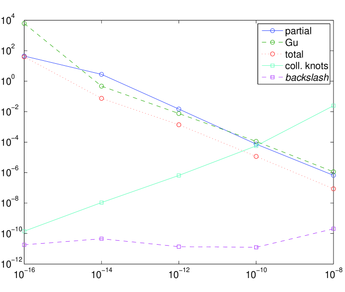
Figure 5: Error in the solution of a Cauchy-like linear system of size 260 with almost multiple knots. Each knot is repeated 5 times, with a different random perturbation producing a relative error less than $\tau$; the values of $\tau$ are reported on the horizontal axis.

Algorithm 3 can be applied to a Cauchy-like matrix with multiple knots; see Section 3.3. We verified that its numerical performance is not influenced by the knots multiplicity and that, when $s_{i}\neq s_{j}$, $\forall i\neq j$, it is roughly as accurate as Algorithm 2, so we prefer to investigate here the particular situation of almost multiple knots. In the script test6.m, we construct a Cauchy-like matrix of size $260$ and displacement rank 5, with random generators. Its knots are obtained starting from 52 equispaced points on the unit circle, and replicating them 4 times, each time with a perturbation producing a relative error less than $\tau$. Figure 5 reports the errors obtained solving the resulting linear system for $\tau=10^{-8},10^{-10},\ldots,10^{-16}$. Our clsolve function was applied with various pivoting techniques; the results labelled as “coll. knots” were obtained by collapsing the knots, i.e., removing the perturbation $\tau$, and then solving the system using Algorithm 4, which includes partial pivoting. In this way, a different system is solved, since the matrix is perturbed, but when $\tau$ tends to zero this approach is much more accurate than Algorithm 2. The condition number of the matrix is about $10^{5}$ for any $\tau$; this fact is confirmed by the results obtained by Matlab backslash.

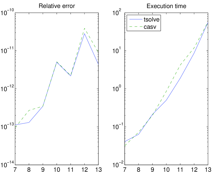
Figure 6: Comparison between tsolve with partial pivoting and the function casv from [24]. Both methods are applied to random real Toeplitz systems of size $2^{k}$, $k=7,\ldots,13$.

While working on this paper, we became aware of another approach to apply the generalized Schur algorithm to a Cauchy-like matrix, using partial pivoting, and requiring $O(n)$ memory locations [24]. As the author kindly sent us the code developed for his paper, we report a comparison of his method and tsolve with partial pivoting. Figure 6 reports the errors and the execution times obtained by applying the Matlab version of both methods to the solution of random real Toeplitz linear systems; the results were computed by suitably modifying the script test2.m. It results that the algorithms are essentially equivalent. Performing the same test using the compiled versions of both methods produces the same errors, but our implementation appears to run faster. We believe that this is due to a different level of code optimization.

References

- [1] E. Anderson, Z. Bai, C. Bischof, J. Demmel, J. Dongarra, J. Du Croz, A. Greenbaum, S. Hammarling, A. McKenney, S. Ostrouchov, and D. Sorensen. LAPACK Users’ Guide. SIAM, Philadelphia, 1992.
-
[2]
A. Aricò and G. Rodriguez.
toms729gw: a Matlab (Fortran) MEX Gateway for TOMS
Algorithm 729, by P. C. Hansen and T. Chan.
University of Cagliari, 2008.
Available at: http://bugs.unica.it/~gppe/soft/. - [3] O. B. Arushanian, M. K. Samarin, V. V. Voevodin, E. Tyrtyshnikov, B. S. Garbow, J. M. Boyle, W. R. Cowell, and K. W. Dritz. The TOEPLITZ Package Users’ Guide. Technical Report ANL-83-16, Argonne National Laboratory, 1983.
- [4] R. H. Bartels, G. H. Golub, and M. A. Saunders. Numerical techniques in mathematical programming. In Nonlinear Programming (Proc. Sympos., Univ. of Wisconsin, Madison, Wis., 1970), pages 123–176. Academic Press, New York, 1970.
- [5] D.A. Bini and P. Boito. A fast algorithm for approximate polynomial gcd based on structured matrix computations. In Numerical Methods for Structured Matrices and Applications: Georg Heinig memorial volume. Birkhäuser, Basel, 2010. To appear.
- [6] Å. Björck. Pivoting and stability in the augmented system method. In Numerical Analysis 1991 (Dundee, 1991), volume 260 of Pitman Res. Notes Math. Ser., pages 1–16. Longman Sci. Tech., Harlow, 1992.
- [7] L. S. Blackford, J. Demmel, J. Dongarra, I. Duff, S. Hammarling, G. Henry, M. Heroux, and L. Kaufman. An updated set of basic linear algebra subprograms (BLAS). ACM Trans. Math. Software, 28(2):135–151, 2002.
- [8] D. Calvetti and L. Reichel. Factorizations of Cauchy matrices. J. Comput. Appl. Math., 86(1):103–123, 1997.
- [9] B. Friedlander, M. Morf, T. Kailath, and L. Ljung. New inversion formulas for matrices classified in terms of their distance from Toeplitz matrices. Linear Algebra Appl., 27:31–60, 1979.
- [10] I. Gohberg, T. Kailath, and V. Olshevsky. Fast Gaussian elimination with partial pivoting for matrices with displacement structure. Math. Comp., 64(212):1557–1576, 1995.
- [11] M. Gu. Stable and efficient algorithms for structured systems of linear equations. SIAM J. Matrix Anal. Appl., 19(2):279–306, 1998.
- [12] P. C. Hansen and T. F. Chan. Fortran subroutines for general Toeplitz systems. ACM Trans. Math. Software, 18(3):256–273, 1992.
- [13] G. Heinig. Inversion of generalized Cauchy matrices and other classes of structured matrices. In Linear Algebra for Signal Processing (Minneapolis, MN, 1992), volume 69 of IMA Vol. Math. Appl., pages 63–81. Springer, New York, 1995.
- [14] G. Heinig and A. Bojanczyk. Transformation techniques for Toeplitz and Toeplitz-plus-Hankel matrices. I. Transformations. Linear Algebra Appl., 254:193–226, 1997.
- [15] G. Heinig and A. Bojanczyk. Transformation techniques for Toeplitz and Toeplitz-plus-Hankel matrices. II. Algorithms. Linear Algebra Appl., 278(1-3):11–36, 1998.
- [16] G. Heinig and K. Rost. Algebraic Methods for Toeplitz-Like Matrices and Operators, volume 13 of Operator Theory: Advances and Applications. Birkhäuser Verlag, Basel, 1984.
- [17] T. Kailath and J. Chun. Generalized displacement structure for block-Toeplitz, Toeplitz-block, and Toeplitz-derived matrices. SIAM J. Matrix Anal. Appl., 15(1):114–128, 1994.
- [18] T. Kailath, S. Y. Kung, and M. Morf. Displacement ranks of matrices and linear equations. J. Math. Anal. Appl., 68(2):395–407, 1979.
- [19] T. Kailath and A. H. Sayed. Displacement structure: theory and applications. SIAM Rev., 37(3):297–386, 1995.
- [20] T. Kailath and A. H. Sayed, editors. Fast Reliable Algorithms for Matrices with Structure, Philadelphia, PA, 1999. Society for Industrial and Applied Mathematics (SIAM).
-
[21]
Katholieke Universiteit Leuven, Department of Computer Science.
MaSe-Team (Matrices having Structure), 2010.
Available at: http://www.cs.kuleuven.ac.be/~marc/software/. - [22] The MathWorks, Natick. Matlab ver. 7.9, 2009.
- [23] C.V.M. van der Mee and S. Seatzu. A method for generating infinite positive self-adjoint test matrices and Riesz bases. SIAM Journal on Matrix Analysis and Applications, 26(4):1132–1149, 2005.
- [24] F. Poloni. A note on the -storage implementation of the GKO algorithm and its adaptation to Trummer-like matrices. Numer. Algorithms, 2010. To appear.
- [25] G. Rodriguez. Fast solution of Toeplitz- and Cauchy-like least-squares problems. SIAM J. Matrix Anal. Appl., 28(3):724–748 (electronic), 2006.
- [26] I. H. Siegel. Deferment of computation in the method of least squares. Math. Comp., 19:329–331, 1965.
-
[27]
SourceForge.net.
Gnumex, 2000.
Available at: http://gnumex.sourceforge.net/. -
[28]
SourceForge.net.
MinGW, 2008.
Available at: http://www.mingw.org/. - [29] D. R. Sweet and R. P. Brent. Error analysis of a fast partial pivoting method for structured matrices. In F. T. Luk, editor, Advanced Signal Processing Algorithms, volume 2563, pages 266–280, San Diego, 1995. SPIE.
-
[30]
University of Pisa, Department of Mathematics.
Structured matrix analysis: numerical methods and applications,
2010.
Available at: http://bezout.dm.unipi.it/.