CUDA simulations of active dumbbell suspensions

Abstract

We describe and analyze CUDA simulations of hydrodynamic interactions in active dumbbell suspensions. GPU-based parallel computing enables us not only to study the time-resolved collective dynamics of up to a several hundred active dumbbell swimmers but also to test the accuracy of effective time-averaged models. Our numerical results suggest that the stroke-averaged model yields a relatively accurate description down to distances of only a few times the dumbbell’s length. This is remarkable in view of the fact that the stroke-averaged model is based on a far-field expansion. Thus, our analysis confirms that stroke-averaged far-field equations of motion may provide a useful starting point for the derivation of hydrodynamic field equations.

I Introduction

The derivation of effective hydrodynamic equations from microscopic or mesoscopic models presents a key problem of non-equilibrium statistical physics 2005ToYuRa . Standard techniques typically involve severe approximations such as, for example, factorization of correlation functions, truncation of hierarchies, closure conditions, etc. Understanding the details of such approximations is crucial for identifying the range of applicability of the resulting field equations. If a complex fluid is made up of active constituents (e.g., bacteria or other micro-organisms) that propel themselves by quasi-periodic swimming mechanisms 1977Pu ; 2009HaMa , then one usually faces the additional task of approximating the explicitly time-dependent microscopic dynamics with a set of coarse-grained, time-averaged equations of motion. Aiming at a better quantitative understanding of this commonly employed approximation, the present paper provides a detailed comparison between the microscopic dynamics of actively driven, spring-based dumbbells and those of a time-averaged analytic model derived from far-field expansion 2008LaBa ; 2008AlYe .

Owing to the fact that hydrodynamic interactions are long-range, simulations of the full time-resolved dynamics of $S=N/2$ dumbbells (each consisting of two spheres) are numerically expensive, scaling as $N^{2}$. However, in the deterministic limit case and/or additive noise limit 1982HaTh , the dynamics is well suited to parallel computations. Very recently, GPU-based codes have been used for various statistical mechanics problems, yielding speed-ups on the order of 20-100 times a CPU-only solution 2009GeEtAl ; 2009PrEtAl ; 2009JaKo ; 2009ThEtAl . Here, we implement a straightforward $N^{2}$ solution of the hydrodynamic equations of motion, a communications-intensive task which is difficult to parallelize in traditional clusters. For a moderate population size (up to a few thousand particles), this method decreases the computation time by a factor of 100 compared with conventional CPU simulations on standard consumer hardware. Hence, we identify GPU computing as a promising approach for future simulations of active particle suspensions (details of the numerical implementation are summarized in Sec. V).

Passive (non-driven) dumbbell models have been widely investigated in polymer science and related fields over the past decades (see, e.g., Refs. 1969Da ; 1982TaZa ; 1989Oet ; 1993AlFr ; 2007SeNe ; 2008BaScZi ; 2008SuLiGe ). Very recently, several authors 2008LaBa ; 2008AlYe ; 2009BaMaPNAS considered active, internally driven dumbbells as prototype systems for collective swimming at zero Reynolds number, $\mathcal{R}=0$. Loosely speaking, one can say that active dumbbell systems constitute a sort of ‘Ising model’ of collective swimming, i.e., they represent strongly simplified models which can be treated by analytical means, thus providing useful insights. Active dumbbells are particularly well-suited to identifying the role of hydrodynamic long-range interactions in collective micro-swimming. This is because isolated deterministic dumbbells are prevented from self-motility by Purcell’s scallop theorem 1977Pu . Hence, any effective motion in deterministic dumbbell systems is caused by hydrodynamic interactions between different dumbbells.

In a recent paper, Alexander and Yeomans 2008AlYe have derived analytical expressions for the effective far-field interactions of symmetric, active dumbbells in three dimensions (3d). Specifically, they showed that the effective hydrodynamic pair interaction decays with distance $|D|$ as $|D|^{-4}$. Considering 1d motions, Lauga and Bartolo 2008LaBa extended this result to asymmetric dumbbells and found that in this case the hydrodynamic interaction decays less strongly as $|D|^{-3}$. While these studies have led to novel insights into interplay between swimmer symmetry and effective long-distance interaction scaling, a detailed comparison of microscopic and stroke-averaged models is still lacking. The present paper intends to close this gap with respect to symmetric dumbbells.

For this purpose, we shall first introduce a microscopic spring-based dumbbell model (Sec. II) that can be readily implemented in GPU-based computer simulations. In the limit of an infinitely stiff spring, our model reduces to a shape-driven dumbbell model as considered in Refs. 2008LaBa ; 2008AlYe . The corresponding 3d stroke-averaged equations of motion will be discussed in Sec. III. After having confirmed that the stroke-averaged model reproduces the main features of the microscopic model simulations in 1d, we perform similar comparative studies for 3d arrays of symmetric dumbbells. Generally, we find that the stroke-averaged dynamics yields relatively accurate description of the microscopic model down to distances of only a few times the dumbbells’ length. This is remarkable in view of the fact that the stroke-averaged model is based on a far-field expansion. Thus, at least for the model considered here, our results suggest that stroke-averaged far-field interaction models may indeed provide a useful starting point for the derivation of hydrodynamic field equations.

II Microscopic modeling of active dumbbells

We shall begin by summarizing the “microscopic” model equations of the spring-based dumbbells simulated in our computer experiments. The corresponding stroke-averaged equations of motion will be discussed in Sec. III. To keep the discussion in this part as general as possible – and as reference for future work – we shall formulate the model for “Brownian” dumbbells, even though the discussion in the subsequent sections will be restricted to the deterministic limit.

We consider a system of $S$ identical dumbbells. Each dumbbell consists of two spheres, of radius $a$. At very low Reynolds numbers, inertia is negligible and the state of the system at time $t$ is completely described by the spheres’ position coordinates $\{\boldsymbol{X}_{\alpha}\}=\{X_{(\alpha i)}(t)\}$ with $\alpha=1,\ldots,2S$ labeling the spheres, and $i=1,2,3$ the space dimension (throughout, we adopt the Einstein summation convention for repeated lower Latin indices). Neglecting rotations of the spheres, the dynamics is governed by the Ito-Langevin equations 1972MuAg ; 1976Bi ; 2009DuLa ; 2003LiDu ; 2007SeNe ; 2009DuZa

$$\dot{X}_{(\alpha i)}(t) = \sum_{\beta}\mathcal{H}_{(\alpha i)(\beta j)}F_{(\beta j)}+$$ (1a)

$$\sum_{\beta}(k_{B}\mathcal{T})^{1/2}C_{(\alpha i)(\beta k)}\,\xi_{(\beta k)}(t),$$

where $$k_{B} \mathcal{T} \dot{X}:=\mathrm{d}X/\mathrm{d}t \xi_{(\gamma k)}(t)$$ denotes the Boltzmann constant and the temperature of the surrounding fluid (). Equation (1a) corresponds to the overdamped limit of Stokesian dynamics 1988BrBo . The Gaussian white noise models stochastic interactions with the surrounding liquid molecules and is characterized by 1998GaHaJuMa

$$\langle\xi_{(\alpha i)}(t)\rangle = 0,$$ (1b)

$$\langle\xi_{(\alpha i)}(t)\xi_{(\beta j)}(t^{\prime})\rangle = \delta_{\alpha\beta}\,\delta_{ij}\,\delta(t-t^{\prime}).$$ (1c)

The hydrodynamic interaction tensor $\mathcal{H}$ couples the deterministic force components $F_{(\beta i)}$ that act on the individual spheres. Generally, the vector $F=\{F_{(\beta i)}\}$ comprises contributions from internal forces, e.g., those required to bind and oscillate spheres in an active dumbbell, as well as from external force fields (gravity, etc.).

The amplitude of the noise force is determined by the fluctuation dissipation theorem, which is satisfied if $C$ is constructed from $\mathcal{H}$ by Cholesky decomposition, i.e.,

$$2\mathcal{H}_{(\alpha i)(\beta j)}=\sum_{\gamma}C_{(\alpha i)(\gamma k)}C_{(\beta j)(\gamma k)}.$$ (2)

In our numerical simulations, $\mathcal{H}$ is given by the Rotne-Prager-Yamakawa-Mazur tensor 1969RoPr ; 1970Ya ; Oseen ; HappelBrenner ; 1982Ma

$$\mathcal{H}_{(\alpha i)(\alpha j)} = \frac{\delta_{ij}}{\gamma_{\alpha}}=\frac{\delta_{ij}}{6\pi\mu a_{\alpha}}$$ (3a)

$$\mathcal{H}_{(\alpha i)(\beta j)} = \frac{1}{8\pi\mu\,r_{\alpha\beta}}\biggl{(}\delta_{ij}+\frac{r_{\alpha\beta i}r_{\alpha\beta j}}{r_{\alpha\beta}^{2}}\biggr{)}+$$ (3b)

$$\frac{2a^{2}}{24\pi\mu\;r_{\alpha\beta}^{3}}\biggl{(}\delta_{ij}-3\frac{r_{\alpha\beta i}r_{\alpha\beta j}}{r_{\alpha\beta}^{2}}\biggr{)},\qquad$$

where $r_{\alpha\beta i}:=x_{\alpha i}-x_{\beta i}$, $\alpha\neq\beta$, and $r_{\alpha\beta}:=|\boldsymbol{x}_{\alpha}-\boldsymbol{x}_{\beta}|$. Analytical formulas presented below are based on an Oseen approximation, which neglects the second line in Eq. (3b). The diagonal components (3a) describe Stokesian friction in a fluid of viscosity $\mu$. The off-diagonal components (3b) model hydrodynamic interactions between different spheres. Note that $\mathcal{H}$ is positive definite for $r_{\alpha\beta}>2a$ and divergence-free, $\partial_{(\beta j)}\mathcal{H}_{(\alpha i)(\beta j)}\equiv 0$ with $\partial_{(\beta i)}:=\partial/\partial x_{(\beta i)}$, implying that the Cholesky-decomposition (2) is well-defined.

To completely specify the model, we still need to fix the intra-dumbbell force. To this end, consider the dumbbell $\sigma$, formed by spheres $\alpha=2\sigma-1$ and $\beta=2\sigma$, and denote its length by $d^{\sigma}(t):=|\boldsymbol{X}_{\beta}(t)-\boldsymbol{X}_{\alpha}(t)|$. Neglecting external force fields from now on, we shall assume that the two spheres are connected by a harmonic spring of variable length $L^{\sigma}(t)$, i.e., $F_{(\beta i)}=-\partial_{(\beta i)}U$ where

$$U=\sum_{\sigma}U^{\sigma},\qquad U^{\sigma}(t,d^{\sigma})=\frac{k_{0}}{2}\,[d^{\sigma}-L^{\sigma}(t)]^{2},\;$$

with $L^{\sigma}(t)=\ell+\lambda\sin(\omega t+\varphi^{\sigma})$ denoting the time-dependent equilibrium length of the spring, and $\ell$ the mean length such that $\ell>2a+\lambda$. The dumbbell swimmer is called passive if the stroke amplitude $\lambda=0$, and active if $|\lambda|>0$. As discussed below, the phase parameter $\varphi^{\sigma}$ is important for the interaction between two or more dumbbells.

For the overdamped description (1) to remain valid, the driving must be sufficiently slow. More precisely, we have to impose that $T_{\gamma}\ll T_{0}\ll T$, where $T:=2\pi/\omega$ is the driving period, $T_{0}:=2\pi/\sqrt{k_{0}/M}$ the oscillator period for a sphere of mass $M$, and $T_{\gamma}:=M/\gamma$ the characteristic damping time. This restriction ensures that the dumbbells behave similar to shape-driven swimmers, i.e., $d^{\sigma}\simeq L^{\sigma}(t)$ is a useful approximation in analytical calculations.

With the above assumptions, the $N$-particle PDF $f(t,\{x_{(\alpha i)}\})$ of the stochastic process $\{X_{(\alpha i)}(t)\}$ from Eq. (1) is governed by the Kirkwood-Smoluchowski equation

$$\partial_{t}f=\sum_{\alpha,\beta}\partial_{(\alpha i)}\mathcal{H}_{(\alpha i)(\beta j)}\left\{\left[\partial_{(\beta j)}U\right]f+k_{B}\mathcal{T}\partial_{(\beta j)}f\right\}.$$ (5)

For time-independent potentials, the stationary solution of this equation is given by the Boltzmann distribution, $f\propto~{}e^{-U/(k_{B}\mathcal{T})}$. However, in the remainder, we shall focus on the deterministic limit case, formally obtained by putting $\mathcal{T}=0$ in Eqs. (1a), which is justified for sufficiently big spheres.

III Stroke-averaged hydrodynamic pair interactions

In this part we will summarize the stroke-averaged equations of motion for the case of 3d symmetric, deterministic dumbbell swimmers (a detailed derivation, which differs slightly from that in Ref. 2008AlYe but yields equivalent results, is given in the Appendix). In Sec. IV, the dynamics resulting from these effective equations of motion for the dumbbell positions and orientations will be compared with numerical simulations of the microscopic model equations (1). From now on all consideration refers to the deterministic limit case.

III.1 General stroke-averaging procedure

We characterize each dumbbell by its direction vector

$$\tilde{\boldsymbol{N}}^{\sigma}(t)=\frac{\boldsymbol{X}_{2\sigma}-\boldsymbol{X}_{2\sigma-1}}{|\boldsymbol{X}_{2\sigma}-\boldsymbol{X}_{2\sigma-1}|},\qquad\sigma=1,\ldots,S$$ (6a)

and its geometric center

$$\tilde{\boldsymbol{R}}^{\sigma}(t):=\frac{1}{2}\left(\boldsymbol{X}_{2\sigma}+\boldsymbol{X}_{2\sigma-1}\right).$$ (6b)

Note that for symmetric dumbbells the geometric center coincides with the center of hydrodynamic stress HappelBrenner ; 2009BaMaPNAS .

The basic idea of the stroke-averaging procedure 2008LaBa ; 2008AlYe ; 2009DuZa is to focus on the dynamics of averaged position and orientation coordinates $\boldsymbol{R}(t)$ and $\boldsymbol{N}^{\sigma}(t)$, which are defined by

$$\boldsymbol{N}^{\sigma}(t) := \frac{1}{T}\int_{t-T/2}^{t+T/2}\mathrm{d}u\;\tilde{\boldsymbol{N}}^{\sigma}(u),$$ (7a)

$$\boldsymbol{R}^{\sigma}(t) := \frac{1}{T}\int_{t-T/2}^{t+T/2}\mathrm{d}u\;\tilde{\boldsymbol{R}}^{\sigma}(u).$$ (7b)

Here $T=2\pi/\omega$ denotes the period of a swimming stroke. By assuming that $\tilde{\boldsymbol{N}}^{\sigma}(t)$ and $\tilde{\boldsymbol{R}}^{\sigma}(t)$ are slowly varying functions of time, one can further approximate

$$\dot{\boldsymbol{N}}^{\sigma}\simeq\dot{\tilde{\boldsymbol{N}}}^{\sigma}\;,\qquad\dot{\boldsymbol{R}}^{\sigma}\simeq\dot{\tilde{\boldsymbol{R}}}^{\sigma},\quad\qquad\qquad$$ (8a)

$$\frac{1}{T}\int_{t-T/2}^{t+T/2}\!\!\!\!\mathrm{d}s\;f(\tilde{\boldsymbol{N}}^{\sigma}(s),\tilde{\boldsymbol{R}}^{\sigma}(s))\simeq f({\boldsymbol{N}}^{\sigma}(t),{\boldsymbol{R}}^{\sigma}(t))$$ (8b)

for any sufficiently well-behaved function $f$.

III.2 Stroke-averaged equations of motion

Using the approximations (8), one can derive from the microscopic model equations (1) with $\mathcal{T}=0$ the corresponding deterministic, stroke-averaged, far-field equations of motion 2008LaBa ; 2008AlYe ; 2009DuZa , by making the following simplifying assumptions:

• The dumbbells are force-free and torque-free and approximately shape-driven, i.e.,  $d^{\sigma}:=|\boldsymbol{X}_{2\sigma}-\boldsymbol{X}_{2\sigma-1}|\simeq\ell+\lambda\sin(\omega t+\varphi^{\sigma})$.

• The dumbbells are slender, i.e., sphere radius $a$ and stroke amplitude $\lambda$ have about the same size, but are much smaller than the dumbbell’s mean length $\ell$.

• The ensemble is dilute, meaning that the distance $D^{\sigma\rho}:=|\boldsymbol{D}^{\sigma\rho}|:=|\boldsymbol{R}^{\sigma}-\boldsymbol{R}^{\rho}|$ between dumbbells $\sigma$ and $\rho$ is much larger than $\ell$.

Adopting (i)–(iii) and restricting to two-body interactions, one finds the effective equations of motion

$$\dot{R}_{i}^{\sigma} = \sum_{\rho\neq\sigma}J^{\sigma\rho}_{i},\qquad$$ (9a)

$$\dot{N}_{i}^{\sigma} = -(\delta_{ik}-N^{\sigma}_{i}N^{\sigma}_{k})\;\sum_{\rho\neq\sigma}K^{\sigma\rho}_{k},$$ (9b)

where the stroke-averaged hydrodynamic interaction terms to leading order in $$\lambda/\ell$$ are given by

$$J^{\sigma\rho}_{i} = a\omega\,\sin(\varphi^{\sigma}-\varphi^{\rho})\;\frac{9}{64}\left(\frac{\lambda}{\ell}\right)^{2}\left(\frac{\ell}{|\boldsymbol{D}^{\sigma\rho}|}\right)^{4}\times$$

$$\bigl{\{}N^{\sigma}_{i}(2s+4qr-10sr^{2})+$$

$$\;\;\hat{D}_{i}^{\sigma\rho}(1+2q^{2}-5s^{2}-5r^{2}$$

$$\;\;\;\;-20qsr+35s^{2}r^{2})\bigr{\}},$$

$$K^{\sigma\rho}_{k} = \omega\sin(\varphi^{\sigma}-\varphi^{\rho})\;\frac{15}{64}\left(\frac{a}{\ell}\right)\left(\frac{\lambda}{\ell}\right)^{2}\left(\frac{\ell}{|\boldsymbol{D}^{\sigma\rho}|}\right)^{5}\times$$

$$\;\hat{D}_{k}^{\sigma\rho}\bigl{(}3s+6rq+6sq^{2}-7s^{3}$$

$$\;\;\;-21sr^{2}-42qs^{2}r+63s^{3}r^{2}\bigr{)}.$$

Here, the unit vector $$\hat{\boldsymbol{D}}^{\sigma\rho}:={\boldsymbol{D}^{\sigma\rho}}/{|\boldsymbol{D}^{\sigma\rho}|} \boldsymbol{D}^{\sigma\rho}=\boldsymbol{R}^{\sigma}-\boldsymbol{R}^{\rho} s,r,q$$ gives the orientation of the distance vector , and abbreviate the projections

$$s:=\hat{D}_{j}^{\sigma\rho}N_{j}^{\sigma},\quad r:=\hat{D}_{j}^{\sigma\rho}N_{j}^{\rho},\quad q:=N^{\sigma}_{j}N^{\rho}_{j}.\quad$$ (9d)

One readily observes the following prominent features: (i) The effective translational interactions scale as $\propto|\boldsymbol{D}^{\sigma\rho}|^{-4}$. (ii) The effective rotational interactions scale as $\propto|\boldsymbol{D}^{\sigma\rho}|^{-5}$. (iii) The stroke-averaged interaction terms $J,K$ vanish if the phases $\varphi^{\sigma}$ and $\varphi^{\rho}$ differ by multiples of $\pi$ 2008AlYe . This illustrates the importance of phase (de)tuning in the collective swimming at zero Reynolds number.

IV Microscopic vs. stroke-averaged dynamics

We next compare the predictions of the stroke-averaged equations (9) with numerical results obtained from CUDA simulations of the microscopic spring-based dumbbell model from Sec. II. For this purpose, we first consider 1d aligned dumbbell pairs similar to those studied by Lauga and Bartolo 2008LaBa . The rotational interaction of two dumbbells will be analyzed in Sec. IV.2. Finally, we also study the collective motion of 3d grids of dumbbells (Sec. IV.3). In all cases, the swimmers are assumed to be in an infinite body of fluid initially at rest, i.e., no additional boundary conditions (periodic or otherwise) are imposed.

IV.1 Aligned dumbbell pairs

As long as thermal fluctuations are negligible, aligned dumbbells do not change their orientation and Eq. (9a) reduces to (see  A.1 for an explicit derivation)

$$\dot{R}^{\sigma}=\frac{9}{16}a\omega\sum_{\rho\neq\sigma}\sin(\varphi^{\sigma}-\varphi^{\rho})\;\left(\frac{\lambda}{\ell}\right)^{2}\biggl{(}\frac{\ell}{|D^{\sigma\rho}|}\biggr{)}^{4}\hat{D}^{\sigma\rho},$$

(10)

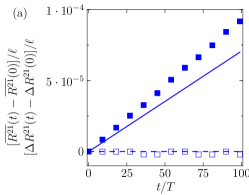
where $\dot{R}^{\sigma}$ denotes the coordinates along the common axis. The lines in Figs. 1 (a) and (b) represent the dynamics of aligned dumbbell pairs ($S=2$) as predicted by Eq. (10). Symbols were obtained from microscopic simulations of the corresponding spring-based model described in Sec. II. Following Lauga and Bartolo 2008LaBa , we quantify collective motion of the dumbbell pairs in terms of their mean collective displacement (solid lines/filled symbols in Fig. 1),

$$\overline{R^{21}}(t)=\frac{1}{2}[R^{2}(t)+R^{1}(t)],\quad$$ (11a)

and their mean relative distance (dashed lines/unfilled symbols in Fig. 1),

$$\Delta R^{21}(t)=R^{2}(t)-R^{1}(t).\quad$$ (11b)

The quantity $\overline{R^{21}}(t)$ characterizes the net motion of the dumbbell pair, whereas $\Delta R^{21}(t)$ indicates whether the dumbbells the move towards or away from each other.

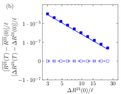
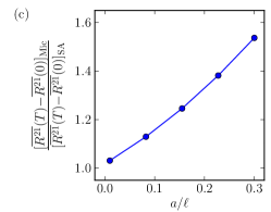
Figure 1: Comparison of exact microscopic motion and effective stroke-averaged dynamics for an aligned dumbbell pair. Lines were obtained by numerical integration of the stroke-averaged equation (10), whereas symbols show the simulation results for the microscopic spring-based dumbbell model described in Sec. II. Solid lines and filled symbols depict the mean displacement $\overline{R^{21}}(t)-\overline{R^{21}}(0)=\{[R^{2}(t)+R^{1}(t)]-[R^{2}(0)+R^{1}(0)]\}/2$ of the geometric centres. Dashed lines and unfilled symbols indicate the relative separation $\Delta R^{21}(t)-\Delta R^{21}(0)=[R^{2}(t)-R^{1}(t)]-[R^{2}(0)-R^{1}(0)]$. (a) Symmetric dumbbells do not change their relative separation and move linearly in time depending on the phase difference $\Delta\varphi=\varphi^{2}-\varphi^{1}$. Simulation parameters are comparable to those of Lauga and Bartolo 2008LaBa : Initial separation $\Delta R^{21}(0)=R^{2}(0)-R^{1}(0)=10\ell$, mean dumbbell length $\ell=5\mu\mathrm{m}$, driving frequency $\omega=500\mathrm{s}^{-1}$ (time on the x-axis is given in units of the stroke period $T=2\pi/\omega$), stroke amplitude $\lambda=0.1\ell$, $a=0.2\ell$, phase difference $\varphi^{2}-\varphi^{1}=\pi/2$. For the microscopic model: spring constants $k_{0}=0.001\mathrm{kg}/\mathrm{s}^{2}$, viscosity $\mu=10^{-3}$ kg/(ms), particle mass density $\varrho=10^{3}$ kg/m³, simulation time step $\Delta t\approx 10^{-4}T$. (b) Distance dependance of the collective motion and separation for aligned dumbbell pairs during a stroke period $T$. Line styles and symbols correspond to the same configurations and simulation parameters as used in (a). Remarkably, the stroke-averaged far-field equation (10) describes the microscopic dumbbell dynamics well down to distances of a few body lengths; however, the deviations from the time-resolved microscopic dynamics accumulate over time, as is evident from (a). The difference between the stroke-averaged dynamics (solid lines) and the microscopic simulations (symbols) in (a) and (b) is due to the choice of a relatively large parameter ratio $a/\ell=0.2$ in these simulations; the results of both methods agree in the limit $a/\ell\to 0$ as illustrated in diagram (c), which shows the ratio of mean swimmer displacements obtained from the microscopic (’Mic’) and stroke-averaged (’SA’) dynamics at constant $\lambda=0.1\ell$ and various choices of $a/\ell$.

.

As is evident from Fig. 1 (a), symmetric dumbbells move in the same direction with identical speeds; the direction of the motion is determined by the phase difference $\varphi^{2}-\varphi^{1}$. As predicted by Eq. (10), the collective displacement over a swimming stroke varies as $|D^{\sigma\rho}|^{-4}$ with the distance between the dumbbells, see Figure 1 (b). Even though the stroke-averaged equations (10) are based on a far-field expansion, they describe the microscopic dynamics of aligned dumbbells well down to distances of a few body lengths.

In this context, it is worthwhile to note that the quantitative difference between the stroke-averaged dynamics (solid lines) and the microscopic simulations (symbols) in Figs. 1 (a) and (b), is due to the relatively large parameter ratio $a/\ell=0.2$ used in these simulations. As shown explicitly in the Appendix, the stroke averaged equations of motion (10) become more accurate in the limit $a/\ell\to 0$. This is confirmed by the numerical results shown in Fig. 1 (c). This diagram depicts the ratio of the average collective swimming speeds (i.e., the collective displacements after a stroke period) obtained by either method for different values of $a/\ell$ at constant stroke-amplitude $\lambda$. We readily observe that this ratio approaches unity in the limit $a/\ell\to 0$. However, in view of the fact that the collective swimming speed is approximately proportional to the sphere radius $a$, see Eq. (10), we opted for a moderate value $a/\ell=0.2$ in all our simulations in order to observe noticeable swimming effects.

IV.2 Two-dimensional rotation of dumbbell pairs

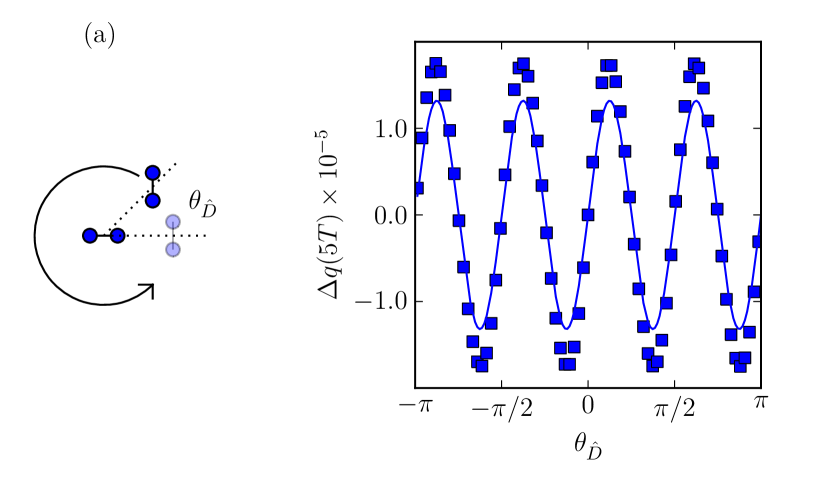
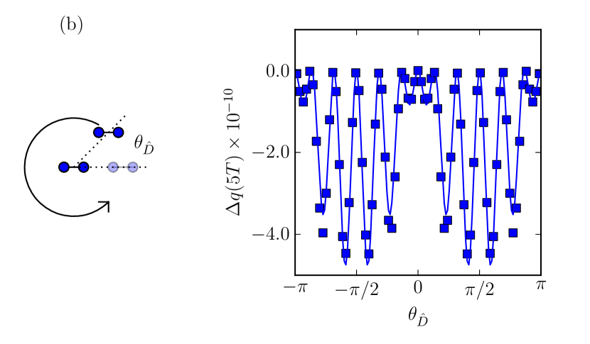
Dumbbells that are arranged in an aligned 1d configuration do not change their orientation. This is different for non-aligned configurations in higher dimensions where hydrodynamic pair interactions can induce rotations. To test the accuracy of the stroke-averaged equation (9b) for the rotational motions in two dimensions, we conducted a series of simulations using the following setup: The first dumbbell (labelled by $\sigma$) was placed at the origin oriented along the $x$-axis, and a second dumbbell ($\rho$) was placed such that the geometric centres were separated by a distance of $5\ell$. By varying the starting position of the second dumbbell along a circle, while keeping the initial projection constant, we can compare numeric and analytic results for various projections $s(t),r(t),q(t)$, as defined in Eq. (9d).

Figure 2 depicts the change of the dumbbells’ relative orientation

$$\Delta q(t):=q(t)-q(0)\;,\qquad q(t):=N^{\sigma}_{j}(t)N^{\rho}_{j}(t)$$ (12)

after five swimming strokes $t=5T$ for two different initial projections (a) $q(0)=0$ and (b) $q(0)=1$. As evident from the diagrams, in both cases the stroke averaged description (9b) correctly reproduces the rotational dynamics of the microscopic spring-based model.

We may thus briefly summarize: The results in Figs. 1 and 2 show that the stroke-averaged equations (9) satisfactorily capture the main features of effective pair interactions in the spring-based microscopic model at moderate-to-low densities (large distances). This corroborates that equations of the type (9) can provide a convenient mesoscopic description which, for example, can be used as a starting point for derivation of coarse-grained macroscopic field theories 2008BaMa . Conversely, the good agreement between the averaged dynamics (9) and the microscopic model simulation provides a helpful confirmation that our CUDA algorithm works correctly even at relatively low densities, when hydrodynamic interactions effects are relatively weak and algorithms may become prone to numerical instabilities.

In the remainder, we shall focus on 3d many-swimmer simulations that fully exploit the virtues of the CUDA parallelization scheme.

Figure 2: Rotational motion of dumbbell pairs; symbols indicate numeric data while lines represent analytics. $\theta_{\hat{D}}$ is the angle between a line connecting the dumbbell’s geometric centres and the $x$-axis; $\Delta q(5T):=q(5T)-q(0)$ where $q(t)$ is the projection of the swimmer orientations $q(t)=N^{1}_{j}(t)N^{2}_{j}(t)$. Initial configurations: (a) $q(0)=0$ and (b) $q(0)=1$ with an initial radial separation of $5\ell$ . One readily observes the good agreement between the microscopic simulations and the analytics.

IV.3 Collective swimming of three-dimensional dumbbell arrays

In this section we will compare the predictions of the stroke-averaged far-field equations (9) with simulations of spring-based dumbbells for 3d dumbbell configurations.

In our simulation the dumbbells’ geometric centers $\boldsymbol{R}^{\sigma}(0)$ are initially placed on a cubic $(x\times x\times x)$-lattice with equidistant spacing $\rho^{-1/3}$, where $\rho$ is the number density of the configuration. Initial orientations $\boldsymbol{N}^{\sigma}(0)$ are sampled uniformly from the unit sphere. For the lattice size we consider values $x=3,5,7,9$ corresponding to a total dumbbell number $S=3^{3},5^{3},7^{3},9^{3}$, respectively. To characterize the collective motion, we measure in our simulations the mean square displacement per particle averaged over different initial conditions, i.e.,

$$\langle\langle R(t)^{2}\rangle\rangle:=\frac{1}{W}\sum^{W}_{w=1}\frac{1}{S}\sum_{\sigma=1}^{S}\left[R^{\sigma}(t;w)-R^{\sigma}(0;w)\right]^{2}$$

where the variable $w=1,\ldots,W$ labels different initial conditions. We distinguish two classes of initial conditions:

• An “optimized” phase distribution: Phases were set such that each dumbbell had a phase of $0$ or $\pi/2$ with all nearest neighbors having the alternate phase in the manner of a 3d “checkerboard”. The corresponding results for the microscopic simulation and the stroke-averaged model are indicated by filled symbols and solid lines in Figs. 3 and 4, respectively.

• A randomized phase distribution: Phases were set to random values evenly distributed on the interval $[0,2\pi)$, with a different distribution for each run. The corresponding results are indicated by unfilled symbols and dashed lines in Figs. 3 and 4, respectively.

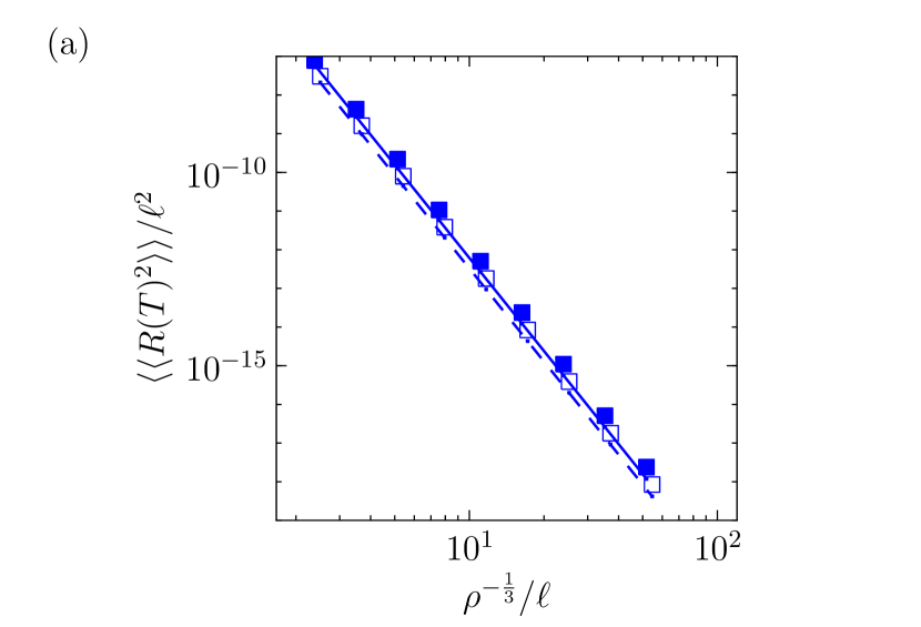
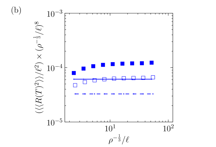
Figure 3: (a) Scaling of the mean square displacement per particle (measured over a period) with number density for two different phase distributions. The diagram depicts the simulation results for a cubic array of $(5\times 5\times 5)=125$ dumbbells, averaged over $W=100$ different runs, each with random initial orientations. Symbols refer to the spring-based model and lines to the stroke-averaged model (9). The collective mean square displacement is proportional to $(\ell\rho^{1/3})^{2\nu}$ with an exponent $\nu=-4$. (b) Mean square displacement rescaled (i.e., multiplied) by $\rho^{-8/3}$. We observe that for an “optimized” phase distribution (filled symbols/solid lines) the effective mean square displacement is larger than for a uniformly random phase distribution (empty symbols/dashed lines). On this scale, statistical error bars (not shown) are smaller than the size of the symbols. The shift between lines and symbols, caused by the relatively large parameter ratio $a/\ell=0.2$ used in these simulations, is consistent with the value expected from Fig. 1 (c).

Fig. 3 illustrates how the mean square displacement over a period, $\langle\langle R(T)^{2}\rangle\rangle$, varies with density $\rho$ – or equivalently with grid spacing – for an array of $(5\times 5\times 5)=125$ dumbbells. As evident from the diagram, the prediction from the stroke-averaged model (9) is in good agreement with the scaling behavior measured for the microscopic model. Furthermore, by comparing filled with unfilled symbols and solid with dashed lines, we note that the collective displacement $\langle\langle R(T)^{2}\rangle\rangle$ is generally smaller for the randomized phase distribution, corroborating the fact that optimizing the phase distributions can considerably enhance the effectiveness of collective motions 2008YaElGo .

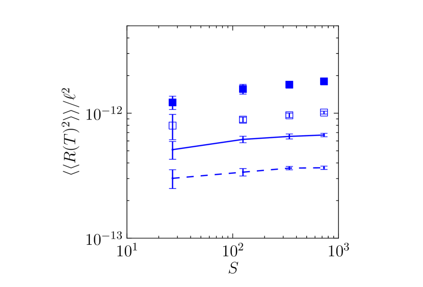
Figure 4 shows how the quantity $\langle\langle R(T)^{2}\rangle\rangle$ scales with the total number $S$ of the dumbbells at fixed density $\rho$. After a slight initial jump from the $(3\times 3\times 3)$ case, adding more swimmers at fixed density $\rho$ produces only a minimal increase in displacement, and the effect appears for both optimized or randomized phase distributions. Again, collective displacement is generally smaller for randomized phase distributions than for optimal phase distributions.

Figure 4: Scaling of the mean square displacement per particle over a period with dumbbell number $S$ at constant density. The diagram depicts the simulation results for collections of dumbbells arranged on a cubic $(x\times x\times x)$-lattice with $x=3,5,7,9$ and spacing $10\ell$, averaged over $W=10$ different random initial orientations. Symbols refer to the spring-based model and lines to the far-field stroke-averaged model (9), beginning from the same initial conditions. Increasing the number of swimmers while keeping the number density constant produces only minimal gains in translational speed. The collective mean square displacement is smallest for $(3\times 3\times 3)=27$ swimmers, which is due to the relatively large number of swimmers with an incomplete set of “nearest neighbors” in this case. We also observe that for an “optimized” phase distribution (filled symbols/solid lines) the effective mean square displacement is larger than for a uniformly random phase distribution (empty symbols/dashed lines). Again, the shift between lines and symbols, caused by the relatively large parameter ratio $a/\ell=0.2$ used in these simulations, is consistent with the value expected from Fig. 1 (c).

V Computational aspects

The numerical results were obtained from parallelized simulations run on graphics processing units (GPUs) using Nvidia’s Compute Unified Device Architecture (CUDA). Compared to conventional CPU programs, GPU algorithms may yield significant speed ups (up to factors of a few hundreds) whenever a problem can be naturally parallelized 2009GeEtAl ; 2009PrEtAl ; 2009JaKo ; 2009ThEtAl , on relatively low-cost consumer-grade hardware. In cases where the problem is small enough to fit on a single device, the resulting software is simpler, easier to test, less costly to implement, and much faster than traditional cluster-based methods. This is the case for deterministic many-swimmer simulations, for stochastic single-swimmer simulations, and also for stochastic many-swimmer simulations with purely additive noise, corresponding to a constant matrix $C$ in Eq. (1).

Most $\mathcal{O}(N^{2})$ problems such as $N$-body simulations with pair interactions involve enough data communication that they are difficult to distribute efficiently, or are costly enough that they must be recast in more numerically tractable forms such as Ewald summation saintillan_smooth_2005 ; brady_stokesian_1988 ; sierou_accelerated_2001 . For cases of a few hundred swimmers, CUDA-based implementations of straightforward $\mathcal{O}(N^{2})$ problems present an excellent method for numerical simulation. We use a simple direct computation of sphere-sphere interactions via the Rotne-Prager-Yamakawa-Mazur tensor, disregarding lubrication forces and close-range interactions due to the dilute nature of the suspensions and slender structure of the dumbbells.

We tested our GPU code on an AMD Phenom X4 940 system running Fedora Linux, using a consumer-level Nvidia GTX 295 GPU and a more research-oriented Tesla C1060 GPU; other tests took place on an Intel i7 860 running Gentoo Linux and a consumer-level GTX 276 GPU. All hardware was capable of double-precision calculation and used version 2.3 of the CUDA toolkit.

Initial testing of a similar but simpler problem (colloids moving under constant applied force, using Oseen interactions and single precision) showed very large benchmarked speed-ups compared with a C-based CPU simulation. For example, with $\sim 2000$ particles, we measured up to a $\sim 450\times$ speed-up when calculating the full hydrodynamic interaction tensor and $\sim 800\times$ speed-up using an un-optimized version of the elegant tiled method described in prins_nbody_2007 . We did not benchmark the current simulation, but estimate the speed-up, while still being significant, to be considerably less due to the complexity of the multi-swimmer problem, additional data transfers from the GPU, and the use of double precision.

Despite the speed advantage of the tiled method, we decided to compute the full hydrodynamic interaction tensor in our simulations, primarily to maintain congruence with existing C code in a battery of automated unit tests and to keep the code as simple as possible. Future implementations will likely reintroduce the tiled calculation to further improve computational efficiency. Generally, it is encouraging that even a relatively straightforward CUDA simulation of the multi-swimmer problem exhibits compelling speed advantages over a CPU-based solution.

The use of double precision is unfortunate in that single precision calculations on CUDA processors show significant performance increases due to better hardware support and memory performance. However, in the case of collective dumbbell motion, the distance moved in each time-step is very small compared to the length of the dumbbells or their position, which caused initial calculations using single precision to fail, as the position incremental during a single timestep fell below the threshold of machine precision. To allow for standardized testing, we elected to use double precision and to accept decreased performance rather than implementing a better accumulation algorithm (such as Kahan summation) based on single precision. For reasons of accuracy, we also chose not to enable Nvidia’s fast-math optimizations. The latter can significantly accelerate the computation of certain numeric functions (particularly trigonometric functions) but this gain comes at the cost of some precision. However, this might represent another opportunity for performance optimization in the future.

Another important issue is the choice of the integrator due to accumulation of errors and the stiffness of the problem. A variety of methods were tested, including Euler, Adams-Bashforth-Moulton, and Runge-Kutta integrators. The approach eventually used was a one-step Heun predictor-corrector method, which produced excellent results and can easily incorporate additive noise for stochastic simulations. The time step for the simulations was chosen based on the smallest dynamical time scale in the problem (given by the spring frequency $T_{0}=2\pi/\sqrt{k_{0}/M}$, see discussion in Sec. II) and then manually reduced until numerical errors were acceptable by ensuring that single dumbbells did not translate and numeric fluctuations were orders of magnitude below the expected motion caused due to hydrodynamic interactions.

The use of a spring-based model created an additional complication: After prescribing the initial position, orientation, and phase of the dumbbell we initially placed the spheres centred at the potential minima. However, numerical integration and finite potential strengths caused the sphere positions to lag very slightly behind the potentials once they began moving periodically. Since the hydrodynamically induced dumbbell motion is of a very small scale compared to the dumbbell size, this initial settling caused a large anomalous motion during the first period of simulation. To rectify this, it was necessary to discard the first period and begin measurements after the lag was established and dumbbell translation was approximately linear. This did cause miniscule deviations of the dumbbells’ mean length $\ell$, amplitude $\lambda$, and phase $\varphi$ from the values specified by the initial conditions, but tuning the potential spring constant to be sufficiently stiff reduced these deviations to acceptable values of a few percent.

While the results shown here are purely deterministic, incorporating noise is relatively straightforward, as the system hydrodynamic tensor $\mathcal{H}$ may be numerically decomposed via Cholesky decomposition 2006Jung ; 2008VoDe . However, even with GPU acceleration this decomposition is prohibitively expensive; in the case of slender dumbbells and dilute suspensions, we advocate a simple additive noise with a constant matrix $C$ as a reasonable approximation in the dilute limit as the off-diagonal terms in Eq. (3) are negligible. We compared the full Cholesky decomposition and an additive-noise approximation in various test runs and found that the results for the collective mean square displacement differed by only a few percent.

VI Conclusions

We have examined the stroke-averaged, far-field equations of motion for symmetric dumbbells, and verified the general properties of this coarse-grained model by comparing with microscopic numerical simulations at relatively low densities. Remarkably, the microscopic and coarse-grained simulations agree well even at intermediate-to-high swimmer densities, where the effective equations of motion are expected to become less accurate. However, it should be kept in mind that at very high densities, when collisions (i.e., steric effects) become relevant, lubrication effects as well as near-field hydrodynamics must be modelled more carefully.

In the case of dumbbells arranged on a 3d grid, the translational speed due to hydrodynamic interaction between dumbbells varies predictably with spacing, tending toward $|D|^{-4}$ decay, where $|D|$ is the distance between dumbbell centres. Due the short range of the effective hydrodynamic interactions for symmetric dumbbells, adding more swimmers at a fixed density has only a minimal impact on dumbbell translational speed. On the other hand, the collective swimming speed can be noticeably increased by replacing a randomized phase distribution with an ordered, “optimal” distribution of phases such that the difference in phase between a periodically-driven dumbbell and its nearest neighbors is $\pi/2$.

Generally, our numerical investigations illustrate that GPU-based simulations of multi-swimmer systems can provide a valuable tool for studying collective motions at very low Reynolds number. Moreover, the CUDA algorithm used in our computer experiments can be readily adapted to simulate hydrodynamic interactions between colloids that can be trapped and manipulated by means of optical tweezers 2009LeEtAl . Such theoretical investigations can help to create more efficient micropumps, e.g., by optimizing the phase relations in oscillating arrays of colloids.

Finally, another long-term objective is to compare many-swimmer simulations with predictions of effective field theories 2002Ra . Our above results suggest that the most promising approach towards achieving this goal may be a two-step procedure: (Step 1) One should try to derive stroke-averaged equations of motion that correctly capture the phase dependence on the level of effective two-particle interactions. As our above discussion has shown, such coarse-grained models can correctly reproduce many of the main features of the microscopic model. Thus, it is sufficient for many purposes to implement the coarse-grained equations into a CUDA environment (step 2). Compared to simulations of the full microscopic dynamics, this may reduce the effective simulation time by an additional factor of 100 or more since the analytic stroke-averaging procedure makes it unnecessary to numerically resolve the smallest dynamical time scales in the system. We hope that our analysis may provide useful guidance for future efforts in this direction.

Acknowledgements.–

J. D. would like to thank Peter Hänggi for many stimulating discussions and the most enjoyable collaboration over the past years. This work was supported by the ONR, USA (J.D.). V. P. acknowledges support from the United States Air Force Institute of Technology. The views expressed in this paper are those of the authors and do not reflect the official policy or position of the United States Air Force, Department of Defense, or the U.S. Government.

Appendix A Stroke-averaging

We derive the stroke-averaged effective interactions between two symmetric, quasi-shape-driven dumbbell swimmers. Each dumbbell consists of two spheres of radius $a$. The swimming stroke of an individual dumbbell is assumed to be both force-free and torque-free.

A.1 One-dimensional case

In one space dimension (1d) we denote the position of the spheres belonging to dumbbell $\sigma$ by $X^{\sigma}_{s}$, $s=1,2$. To characterize position and orientation of the dumbbell, we may introduce center-of-mass and relative coordinates by

$$R^{\sigma} = \frac{1}{2}\left(X_{1}^{\sigma}+X_{2}^{\sigma}\right)$$ (14a)

$$S^{\sigma} = X^{\sigma}_{2}-X_{1}^{\sigma}$$ (14b)

$$N^{\sigma} = (X^{\sigma}_{2}-X_{1}^{\sigma})/|X^{\sigma}_{2}-X_{1}^{\sigma}|;$$ (14c)

hence,

$$X_{1}^{\sigma}=R^{\sigma}-S^{\sigma}/2\;,\qquad X_{2}^{\sigma}=R^{\sigma}+S^{\sigma}/2$$ (14d)

which may also be written as

$$X^{\sigma}_{s}=R^{\sigma}+(-1)^{s}\;S^{\sigma}/2.$$ (14e)

Furthermore, we define the vector connecting two swimmers $\sigma$ and $\rho$ by

$$D^{\sigma\rho} := R^{\sigma}-R^{\rho}$$ (15a)

$$\hat{D}^{\sigma\rho} := (R^{\sigma}-R^{\rho})/|R^{\sigma}-R^{\rho}|.$$ (15b)

The force-free constraint for the dumbbell $\sigma$ can be written as

$$F_{1}^{\sigma}=-F_{2}^{\sigma}=:f^{\sigma},$$ (16)

with $F_{s}^{\sigma}$ denoting the internal forces acting on the first and the second sphere during a swimming stroke. Neglecting thermal fluctuations, the 1d equations of motion can be written as

$$\dot{X}^{\sigma}_{s}=\sum_{\rho,r}H^{\sigma\rho}_{sr}F^{\rho}_{r}.$$ (17)

Here, we sum over all swimmers $\rho=1,\ldots,S$ and the spheres $r=1,2$ of each swimmer. Our goal is to derive from Eq. (17) a stroke-averaged effective equation of motion for $R^{\sigma}$ (for shape-driven dumbbells the motion of $S^{\sigma}$ is trivial in 1d).

The “diagonal” components of the hydrodynamic interaction tensor $H$ are given by the inverse Stokes friction coefficient

$$H^{\sigma\sigma}_{ss}=\gamma^{-1}=(6\pi\mu a)^{-1}.$$ (18)

Adopting the Oseen approximation, the “off-diagonal” components ($s\neq r$) read

$$H^{\sigma\sigma}_{sr}=\frac{\kappa}{|S^{\sigma}|}\;,\qquad H^{\sigma\rho}_{sr}=\frac{\kappa}{|X_{s}^{\sigma}-X_{r}^{\rho}|}$$ (19)

where $\kappa=(4\pi\mu)^{-1}$. It is useful to rewrite

$$X_{s}^{\sigma}-X_{r}^{\rho}=D^{\sigma\rho}+Y^{\sigma\rho}_{sr}$$ (20a)

where

$$Y^{\sigma\rho}_{sr}:=\frac{1}{2}[(-1)^{s}\;S^{\sigma}-(-1)^{r}\;S^{\rho}].$$ (20b)

Using the force free condition (16), we obtain from Eq. (17)

$$\dot{R}^{\sigma} = \sum_{\rho}\frac{1}{2}[(H^{\sigma\rho}_{11}-H^{\sigma\rho}_{12})+(H^{\sigma\rho}_{21}-H^{\sigma\rho}_{22})]f^{\rho}$$ (21a)

$$=: \sum_{\rho}A^{\sigma\rho}f^{\rho}$$

and

$$\dot{S}^{\sigma} = \sum_{\rho}[(H^{\sigma\rho}_{21}-H^{\sigma\rho}_{22})-(H^{\sigma\rho}_{11}-H^{\sigma\rho}_{12})]f^{\rho}$$ (21b)

$$=: \sum_{\rho}B^{\sigma\rho}f^{\rho}$$

Considering approximately shape-driven dumbbells, we have

$$S^{\sigma} = L^{\sigma}(t)\,N^{\sigma},$$

$$|S^{\sigma}| = L^{\sigma}(t),$$

$$\dot{S}^{\sigma} = \dot{L}^{\sigma}(t)\,N^{\sigma},$$ (22)

where the periodic function $L^{\sigma}(t)>0$ describes the shape (length) of the dumbbell at time $t$. Hence, inverting (21b) we obtain the force as a function of the shape

$$f^{\rho}=\sum_{\nu}(B^{-1})^{\rho\nu}\dot{L}^{\nu}(t)\,N^{\nu},$$ (23)

where $B^{-1}$ denotes the inverse of the $(S\times S)$-matrix $B:=(B^{\sigma\rho})$ defined in (21b). Substituting this result into Eq. (21a) yields the following closed equations for the position coordinates

$$\dot{R}^{\sigma}=\sum_{\rho,\nu}A^{\sigma\rho}(B^{-1})^{\rho\nu}\dot{L}^{\nu}(t)\,N^{\nu}.$$ (24)

By means of Eqs. (A.1), we can rewrite the off-diagonal components of the Oseen tensor as

$$H^{\sigma\sigma}_{sr}=\frac{\kappa}{L^{\sigma}},\qquad H^{\sigma\rho}_{sr}=\frac{\kappa}{|D^{\sigma\rho}+Y^{\sigma\rho}_{sr}|}$$ (25a)

where

$$Y^{\sigma\rho}_{sr}=\frac{1}{2}[(-1)^{s}\;L^{\sigma}(t)\,N^{\sigma}-(-1)^{r}\;L^{\rho}(t)\,N^{\rho}]$$

For a system consisting of more than two dumbbells ($S>2$), the rhs. of Eq. (23) contains not only two-body, but also three-body, four-body, …, $S$-body contributions. However, focussing only on the dominant two-body contributions, $B:=(B^{\sigma\rho})$ can be exactly inverted and the rhs. of Eq. (24) can be expanded in the low-density limit corresponding to $|D^{\sigma\rho}|\to\infty$. Averaging the resulting power series over a stroke period $[t-T/2,t+T/2]$ as described in Sec. III.1 and keeping only the leading order contribution, we find the following 1d stroke-averaged equation of motion in two-body approximation

$$\dot{R}^{\sigma}\simeq\frac{9}{16}a\omega\sum_{\rho}\sin(\varphi^{\sigma}-\varphi^{\rho})\left(\frac{\lambda}{\ell}\right)^{2}\biggl{(}\frac{\ell}{|D^{\sigma\rho}|}\biggr{)}^{4}\hat{D}^{\sigma\rho}.$$

A.2 Three-dimensional case

In the 3d case, the derivation of stroke-averaged equations becomes more complicated due to the additional rotational degrees of freedom.

As before, we consider a dilute suspension of $\sigma=1,\ldots,N$ geometrically identical dumbbells of prescribed length $L^{\sigma}(t)$. To characterize the motion of the dumbbells, we define position and orientation vectors by

$$\boldsymbol{R}^{\sigma}(t) := \frac{1}{2}(\boldsymbol{X}^{\sigma 1}+\boldsymbol{X}^{\sigma 2})$$

$$\boldsymbol{N}^{\sigma}(t) := \frac{\boldsymbol{S}^{\sigma}}{|\boldsymbol{S}^{\sigma}|},$$ (26)

with $\boldsymbol{S}^{\sigma}$ denoting the non-normalized orientation vector, i.e., for a shape-driven dumbbell we can write

$$\boldsymbol{S}^{\sigma}(t) := \boldsymbol{X}^{\sigma 2}-\boldsymbol{X}^{\sigma 1}=L^{\sigma}(t)\boldsymbol{N}^{\sigma},$$ (27a)

$$S^{\sigma}(t) := |\boldsymbol{S}^{\sigma}|=L^{\sigma}.$$ (27b)

Similar to Eq. (14e), we can recover the bead coordinates $$\{\boldsymbol{X}^{\sigma 1},\boldsymbol{X}^{\sigma 2}\} \{\boldsymbol{R}^{\sigma},\boldsymbol{N}^{\sigma}\}$$ from by means of

$$\boldsymbol{X}^{\sigma s} = \boldsymbol{R}^{\sigma}+(-1)^{s}\boldsymbol{N}^{\sigma}L^{\sigma}/2.$$ (27c)

As before, we consider shape-driven dumbbells with $L^{\sigma}(t)=\ell+\lambda\sin(\omega t+\varphi^{\sigma})$. From the definition (A.2), one then finds that the exact equations of motion for $\{\boldsymbol{R}^{\sigma},\boldsymbol{N}^{\sigma}\}$ are given by

$$\dot{R}^{\sigma}_{i} = \frac{1}{2}\sum_{s,\rho,r}H_{ij}^{(\sigma s)(\rho r)}F^{\rho r}_{j}$$ (28a)

$$\dot{N}_{i}^{\sigma} = (\delta_{ik}-N^{\sigma}_{i}N^{\sigma}_{k})\times$$

$$\frac{1}{L^{\sigma}}\sum_{\rho\neq\sigma,r}\left[H_{kj}^{(\sigma 2)(\rho r)}-H_{kj}^{(\sigma 1)(\rho r)}\right]F^{\rho r}_{j}$$

The indices $s,r\in\{1,2\}$ label the spheres and, throughout, we use the sum convention $H_{ij}F_{j}:=\sum_{j}H_{ij}F_{j}$ for spatial tensor indices. Restricting ourselves to dilute suspensions of slender dumbbells, we adopt the Oseen approximation for the hydrodynamic interaction tensor, i.e.,

$$H^{(\sigma s)(\sigma s)}_{ij} = (6\pi\mu a)^{-1}\delta_{ij},$$ (29a)

$$H^{(\sigma s)(\sigma r)}_{ij} = \frac{\kappa}{L^{\sigma}}\left(\delta_{ij}+N^{\sigma}_{i}N^{\sigma}_{j}\right),$$ (29b)

$$H^{(\sigma s)(\rho r)}_{ij} = \frac{\kappa}{|\boldsymbol{X}^{\sigma s}-\boldsymbol{X}^{\rho r}|}\times$$

$$\left[\delta_{ij}+\frac{(X_{i}^{\sigma s}-X_{i}^{\rho r})(X_{j}^{\sigma s}-X_{j}^{\rho r})}{|\boldsymbol{X}^{\sigma s}-\boldsymbol{X}^{\rho r}|^{2}}\right]$$

where $\kappa=(8\pi\mu)^{-1}$. To obtain from Eqs. (28) closed stroke-averaged equations for $\left\{\boldsymbol{R}^{\sigma},\boldsymbol{N}^{\sigma}\right\}$, we must

• perform a far-field expansion of the hydrodynamic interaction tensor;

• determine the internal forces $\boldsymbol{F}^{\sigma s}$, required to maintain the dumbbells’ prescribed shape $L^{\sigma}(t)$;

• expand the resulting equations in powers of $(\lambda/\ell)$ and average over a stroke period $[t,t+T].$

A.2.1 Far-field expansion

The Oseen tensor components $H_{ij}$ given in Eq. (29) are functions of the sphere separation vectors $\boldsymbol{X}^{\sigma s}-\boldsymbol{X}^{\rho r}$. By means of Eq. (27c), we may decompose

$$\boldsymbol{X}^{\sigma s}-\boldsymbol{X}^{\rho r}=\boldsymbol{D}^{\sigma\rho}+\boldsymbol{Y}^{(\sigma s)(\rho r)},$$ (30)

where similar to Eqs. (25) we have defined

$$\boldsymbol{D}^{\sigma\rho} := \boldsymbol{R}^{\sigma}-\boldsymbol{R}^{\rho},$$ (31a)

$$\boldsymbol{Y}^{(\sigma s)(\rho r)} := \frac{1}{2}\left[(-1)^{s}\boldsymbol{N}^{\sigma}L^{\sigma}-(-1)^{r}\boldsymbol{N}^{\rho}L^{\rho}\right]$$

Then, for $\sigma\neq\rho$, the Oseen tensor components (LABEL:e:Oseen_c) take the form

$$H_{ij}:=\frac{\kappa}{|\boldsymbol{D}+\boldsymbol{Y}|}\biggl{(}\delta_{ij}+\frac{D_{i}+Y_{i}}{|\boldsymbol{D}+\boldsymbol{Y}|}\frac{D_{j}+Y_{j}}{|\boldsymbol{D}+\boldsymbol{Y}|}\biggr{)}.\qquad$$ (32)

For clarity, we dropped superscripts here using the abbreviations $\boldsymbol{Y}:=\boldsymbol{Y}^{(\sigma s)(\rho r)}$ and $\boldsymbol{D}:=\boldsymbol{D}^{\sigma\rho}$. In the dilute limit, corresponding to $|\boldsymbol{Y}|\ll|\boldsymbol{D}|$ we may perform a far-field (Taylor) expansion of the tensor components $H_{ij}$. For this purpose we define

$$H^{0}_{ij}:=H_{ij}(\boldsymbol{Y}=\boldsymbol{0})=\frac{\kappa}{|\boldsymbol{D}|}\left(\delta_{ij}+\hat{D}_{i}\hat{D}_{j}\right),\qquad$$ (33a)

where

$$\hat{D}_{i}:=\frac{D_{i}}{|\boldsymbol{D}|}$$ (33b)

is the unit vector in the direction of $\boldsymbol{D}$. Reinstating upper indices, the formal Taylor expansion of $H^{(\sigma s)(\rho r)}_{ij}$ at $\boldsymbol{Y}=\boldsymbol{0}$ can be expressed as

$$H^{(\sigma s)(\rho r)}_{ij}=\sum_{q=0}^{\infty}H^{\sigma\rho}_{ij,k_{q}...k_{1}}Y^{(\sigma s)(\rho r)}_{k_{1}}\cdots Y^{(\sigma s)(\rho r)}_{k_{q}},$$

where

$$H^{\sigma\rho}_{ij,k_{q}...k_{1}} := \frac{1}{q!}\,\partial_{k_{1}}\cdots\partial_{k_{q}}H^{0}_{ij}\biggl{|}_{\boldsymbol{D}=\boldsymbol{D}^{\sigma\rho}}$$ (34b)

and $\partial_{k_{j}}:=\partial/\partial D_{k_{j}}$. Explicit expressions for the expansion coefficients $H_{ij,k_{q}...k_{1}}$ with $q=1,2,3,4$ are summarized in  B. The expansion (34) will be used in the next part to compute the interaction forces $\boldsymbol{F}^{\sigma s}$, and, later on, it will also be inserted into the exact equations of motion (28).

A.2.2 Internal forces in two-particle approximation

We wish to determine the internal forces $\boldsymbol{F}^{\sigma s}$ in Eq. (28) by means of an iterative procedure, restricting ourselves to two-body interactions and assuming, as usual, that individual dumbbell swimmers are both force-free and torque-free, i.e.,

$$0 \overset{!}{\equiv} \sum_{s}F_{i}^{\sigma s},$$ (35a)

$$0 \overset{!}{\equiv} T^{\sigma}_{i}(\boldsymbol{y}):=\sum_{s}\epsilon_{ijk}(X^{\sigma s}_{j}-y_{j})F^{\sigma s}_{k},\qquad$$ (35b)

where $\boldsymbol{y}=(y_{j})$ is an arbitrary reference point. Substituting Eq. (35a) into Eq. (35b) we find that

$$0\equiv\epsilon_{ijk}(X^{\sigma 1}_{j}-X^{\sigma 2}_{j})F^{\sigma 1}_{k},$$

or equivalently

$$0\equiv\epsilon_{ijk}N^{\sigma}_{j}F^{\sigma 1}_{k}.$$ (36)

This implies that $\boldsymbol{F}^{\sigma s}$ must be of the form

$$\boldsymbol{F}^{\sigma s}=f^{\sigma s}\boldsymbol{N}^{\sigma},\qquad f^{\sigma 2}=-f^{\sigma 1}.$$ (37)

It thus remains to express the $N$ unknown functions $f^{\sigma 1}$ in terms of $\left\{\boldsymbol{R}^{\sigma},\boldsymbol{N}^{\sigma}\right\}$.

Shape-constraints.–

To determine the unknown functions $f^{\sigma 1}$, we exploit the $N$ independent shape constraints

$$\dot{L}^{\sigma}\overset{!}{=}N^{\sigma}_{i}(\dot{X}^{\sigma 2}_{i}-\dot{X}^{\sigma 1}_{i}).$$ (38)

Inserting the equations of motion for $\boldsymbol{X}^{\sigma s}$, we find the explicit condition

$$\dot{L}^{\sigma}\overset{!}{=}\sum_{\rho,r}N^{\sigma}_{i}\left[H_{ij}^{(\sigma 2)(\rho r)}-H_{ij}^{(\sigma 1)(\rho r)}\right]N^{\rho}_{j}\,f^{\rho r}.$$ (39)

Introducing the convenient abbreviation

$$h^{(\sigma s)(\rho r)}:=N^{\sigma}_{i}\;H_{ij}^{(\sigma s)(\rho r)}\,N^{\rho}_{j},$$ (40)

we can write Eq. (39) as

$$\dot{L}^{\sigma} \overset{!}{=} \sum_{r}\left[h^{(\sigma 2)(\sigma r)}-h^{(\sigma 1)(\sigma r)}\right]f^{\sigma r}+$$ (41)

$$\sum_{\rho\neq\sigma,r}\left[h^{(\sigma 2)(\rho r)}-h^{(\sigma 1)(\rho r)}\right]f^{\rho r}.\qquad$$

Here, we have separated interactions within the dumbbell $\sigma$ from those with other swimmers $\rho\neq\sigma$. Using the force-free constraint (37), Eq. (41) takes the form

$$\dot{L}^{\sigma} \overset{!}{=} b^{\sigma\sigma}f^{\sigma 1}+\sum_{\rho\neq\sigma}b^{\sigma\rho}f^{\rho 1},$$ (42a)

with coefficient functions

$$b^{\sigma\rho}:=h^{(\sigma 2)(\rho 1)}+h^{(\sigma 1)(\rho 2)}-[h^{(\sigma 2)(\rho 2)}+h^{(\sigma 1)(\rho 1)}]$$

The $N$ linear equations (42a) determine the $N$ unknown functions $f^{\rho 1}$ by means of an iterative procedure.

Iteration scheme.–

Rewriting Eq. (42a) in the form

$$f^{\sigma 1}=\frac{\dot{L}^{\sigma}}{b^{\sigma\sigma}}-\sum_{\rho\neq\sigma}\frac{b^{\sigma\rho}}{b^{\sigma\sigma}}f^{\rho 1}$$ (43)

we obtain the following recursive sequence

$$f^{\sigma 1}_{(n)}=\frac{\dot{L}^{\sigma}}{b^{\sigma\sigma}}-\sum_{\rho\neq\sigma}\frac{b^{\sigma\rho}}{b^{\sigma\sigma}}f^{\rho 1}_{(n-1)}.$$ (44)

Starting from the initial condition $f^{\rho 1}_{(0)}=0$, the first iteration gives the force generated by an isolated, shape-driven dumbbell

$$f^{\sigma 1}_{(1)}=\frac{\dot{L}^{\sigma}}{b^{\sigma\sigma}}.$$ (45)

The second iteration yields a correction due to pair interactions with other dumbbells,

$$f^{\sigma 1}_{(2)} = \frac{\dot{L}^{\sigma}}{b^{\sigma\sigma}}-\sum_{\rho\neq\sigma}\frac{b^{\sigma\rho}}{b^{\sigma\sigma}}\frac{\dot{L}^{\rho}}{b^{\rho\rho}}$$ (46)

$$= f^{\sigma 1}_{(1)}-\sum_{\rho\neq\sigma}\frac{b^{\sigma\rho}}{b^{\sigma\sigma}}\frac{\dot{L}^{\rho}}{b^{\rho\rho}}.$$

Similarly, one obtains from the third iteration

$$f^{\sigma 1}_{(3)} = \frac{\dot{L}^{\sigma}}{b^{\sigma\sigma}}-\sum_{\rho\neq\sigma}\frac{b^{\sigma\rho}}{b^{\sigma\sigma}}\left[\frac{\dot{L}^{\rho}}{b^{\rho\rho}}-\sum_{\nu\neq\rho}\frac{b^{\rho\nu}}{b^{\rho\rho}}\frac{\dot{\ell}^{\nu}}{b^{\nu\nu}}\right]$$ (47)

$$= f^{\sigma 1}_{(2)}+\sum_{\rho\neq\sigma}\sum_{\nu\neq\rho}\frac{b^{\sigma\rho}}{b^{\sigma\sigma}}\frac{b^{\rho\nu}}{b^{\rho\rho}}\frac{\dot{\ell}^{\nu}}{b^{\nu\nu}}.$$

The last term can be interpreted as a three-particle interaction correction. Let us assume that the system contains $\sigma=1,\ldots,N$ dumbbells. Then, as evident from the ‘exclusive’  summation in Eq. (47), the iteration will approach a fixed point after $N$ iterations,

$$f^{\sigma 1}_{(N+1)}=f^{\sigma 1}_{(N)}.$$ (48)

The fixed point $f_{(N)}$ corresponds to the exact solution, i.e., $f_{(N)}$ is the internal force generated by a dumbbell in order to maintain its prescribed shape in the presence hydrodynamic forces of $N-1$ other dumbbells. In the remainder, we shall restrict ourselves to considering one-particle and two-particle interactions, corresponding to $f^{\sigma 1}_{(1)}$ and $f^{\sigma 1}_{(2)}$.

Coefficients $b^{\sigma\rho}$.–

We still need to determine the coefficients $b^{\sigma\rho}$ from (42). The ’diagonal’ coefficients $b^{\sigma\sigma}$ can be calculated exactly by noting that

$$h^{(\sigma s)(\sigma s)} = (6\pi\mu a)^{-1}=\frac{4\kappa}{3a}$$ (49a)

$$h^{(\sigma 1)(\sigma 2)} = h^{(\sigma 2)(\sigma 1)}\quad=\frac{2\kappa}{L^{\sigma}}$$ (49b)

We thus have

$$b^{\sigma\sigma}=\frac{4\kappa}{L^{\sigma}}\left(1-\frac{2L^{\sigma}}{3a}\right).$$ (50)

In order to determine the coefficients $b^{\sigma\rho}$ with $\rho\neq\sigma$, we need to use the far-field expansion (34). Defining the contraction

$$h^{\sigma\rho}_{k_{q}...k_{1}} := N^{\sigma}_{i}N^{\rho}_{j}\;H^{\sigma\rho}_{ij,k_{q}...k_{1}}$$ (51)

allows us to write

$$b^{\sigma\rho}=\sum_{q=0}^{\infty}b_{q}^{\sigma\rho},$$ (52a)

where

$$b_{q}^{\sigma\rho}=h^{\sigma\rho}_{k_{q}...k_{1}}\times$$

$$\quad\bigl{\{}Y^{(\sigma 1)(\rho 2)}_{k_{1}}\cdots Y^{(\sigma 1)(\rho 2)}_{k_{q}}+Y^{(\sigma 2)(\rho 1)}_{k_{1}}\cdots Y^{(\sigma 2)(\rho 1)}_{k_{q}}-$$

$$\quad\;[Y^{(\sigma 1)(\rho 1)}_{k_{1}}\cdots Y^{(\sigma 1)(\rho 1)}_{k_{q}}+Y^{(\sigma 2)(\rho 2)}_{k_{1}}\cdots Y^{(\sigma 2)(\rho 2)}_{k_{q}}]\bigr{\}}.$$

(52b)

We define

$$N^{\sigma\rho}_{k_{1}k_{2}} := N^{\sigma}_{k_{1}}N^{\rho}_{k_{2}}+N^{\sigma}_{k_{2}}N^{\rho}_{k_{1}}\;,$$ (53a)

$$N^{\sigma\sigma\rho}_{k_{1}k_{2}k_{3}} := N^{\sigma}_{k_{1}}N^{\sigma}_{k_{2}}N^{\rho}_{k_{3}}+N^{\sigma}_{k_{1}}N^{\sigma}_{k_{3}}N^{\rho}_{k_{2}}+$$ (53b)

$$N^{\sigma}_{k_{2}}N^{\sigma}_{k_{3}}N^{\rho}_{k_{1}},$$

$$N^{\sigma\sigma\rho\rho}_{k_{1}k_{2}k_{3}k_{4}} := N^{\sigma}_{k_{1}}N^{\sigma}_{k_{2}}N^{\rho}_{k_{3}}N^{\rho}_{k_{4}}+N^{\sigma}_{k_{1}}N^{\sigma}_{k_{3}}N^{\rho}_{k_{2}}N^{\rho}_{k_{4}}+$$

$$N^{\sigma}_{k_{1}}N^{\sigma}_{k_{4}}N^{\rho}_{k_{2}}N^{\rho}_{k_{3}}+N^{\sigma}_{k_{2}}N^{\sigma}_{k_{3}}N^{\rho}_{k_{1}}N^{\rho}_{k_{4}}+$$

$$N^{\sigma}_{k_{2}}N^{\sigma}_{k_{4}}N^{\rho}_{k_{1}}N^{\rho}_{k_{3}}+N^{\sigma}_{k_{3}}N^{\sigma}_{k_{4}}N^{\rho}_{k_{1}}N^{\rho}_{k_{2}},$$

$$N^{\sigma\sigma\sigma\rho}_{k_{1}k_{2}k_{3}k_{4}} := N^{\sigma}_{k_{1}}N^{\sigma}_{k_{2}}N^{\sigma}_{k_{3}}N^{\rho}_{k_{4}}+N^{\sigma}_{k_{1}}N^{\sigma}_{k_{2}}N^{\sigma}_{k_{4}}N^{\rho}_{k_{3}}+$$

$$N^{\sigma}_{k_{1}}N^{\sigma}_{k_{3}}N^{\sigma}_{k_{4}}N^{\rho}_{k_{2}}+N^{\sigma}_{k_{2}}N^{\sigma}_{k_{3}}N^{\sigma}_{k_{4}}N^{\rho}_{k_{1}}.$$

With these abbreviations we find

$$b^{\sigma\rho}_{0} = 0,$$ (54a)

$$b^{\sigma\rho}_{1} = 0,$$ (54b)

$$b^{\sigma\rho}_{2} = h^{\sigma\rho}_{k_{2}k_{1}}\;L^{\sigma}L^{\rho}\;N^{\sigma\rho}_{k_{1}k_{2}},$$ (54c)

$$b^{\sigma\rho}_{3} = 0,$$ (54d)

$$b^{\sigma\rho}_{4} = \frac{1}{4}h^{\sigma\rho}_{k_{4}k_{3}k_{2}k_{1}}\bigl{[}L^{\sigma}L^{\sigma}L^{\sigma}L^{\rho}\,N^{\sigma\sigma\sigma\rho}_{k_{1}k_{2}k_{3}k_{4}}+$$

$$\qquad\qquad\quad L^{\rho}L^{\rho}L^{\rho}L^{\sigma}\,N^{\rho\rho\rho\sigma}_{k_{1}k_{2}k_{3}k_{4}}\bigr{]},$$

which can be used in (46).

A.2.3 Stroke-averaging

Translational motion.–

Inserting the ansatz (37) into Eq. (28), the motion of the position coordinate is determined by

$$\dot{R}^{\sigma}_{i}=\frac{1}{2}\sum_{s,\rho,r}H_{ij}^{(\sigma s)(\rho r)}f^{\rho r}N^{\rho}_{j}.$$ (55)

It is convenient to consider ‘internal’ and external contributions separately by writing

$$\dot{R}^{\sigma}_{i} = N^{\sigma}_{i}I^{\sigma}+\sum_{\rho\neq\sigma}J^{\sigma\rho}_{i}$$ (56a)

where

$$I^{\sigma} := \frac{1}{2}\sum_{s,r}h^{(\sigma s)(\sigma r)}f^{\sigma r},$$ (56b)

$$J^{\sigma\rho}_{i} := \frac{1}{2}\sum_{s,r}H_{ij}^{(\sigma s)(\rho r)}f^{\rho r}N^{\rho}_{j}.$$ (56c)

Here we have used that

$$H_{ij}^{(\sigma s)(\sigma r)}N^{\sigma}_{j}=h^{(\sigma s)(\sigma r)}N^{\sigma}_{i}.$$

Using the force-free constraint and Eq. (49), we find

$$I^{\sigma}=0,$$ (57)

i.e., the only contribution to the translation of swimmer $\sigma$ comes from interactions with the other dumbbells $\rho\neq\sigma$. Hence, we still need to determine the second contribution $J^{\sigma\rho}_{i}$ from Eq. (56c), which can be written in the form

$$J^{\sigma\rho}_{i}=\Xi^{\sigma\rho}_{ij}\,N^{\rho}_{j}\;f^{\rho 1},$$ (58a)

where

$$\Xi^{\sigma\rho}_{ij} := \frac{1}{2}\bigl{[}H_{ij}^{(\sigma 1)(\rho 1)}-H_{ij}^{(\sigma 1)(\rho 2)}\bigr{]}+$$ (58b)

$$\frac{1}{2}\bigl{[}H_{ij}^{(\sigma 2)(\rho 1)}-H_{ij}^{(\sigma 2)(\rho 2)}\bigr{]}.$$

Inserting the far-field expansion for the Oseen tensor, we obtain

$$\Xi^{\sigma\rho}_{ij}=\sum_{q=0}^{\infty}H^{\sigma\rho}_{ij,k_{q}\ldots k_{1}}\;P^{\sigma\rho}_{k_{1}\ldots k_{q}}(\boldsymbol{Y})$$ (59a)

with polynomials $$P^{\sigma\rho}_{k_{1}\ldots k_{q}}$$ given by

$$P^{\sigma\rho}_{k_{1}\ldots k_{q}}(\boldsymbol{Y}) := \frac{1}{2}Y^{(\sigma 1)(\rho 1)}_{k_{1}}\cdots Y^{(\sigma 1)(\rho 1)}_{k_{q}}-$$ (59b)

$$\frac{1}{2}Y^{(\sigma 1)(\rho 2)}_{k_{1}}\cdots Y^{(\sigma 1)(\rho 2)}_{k_{q}}+$$

$$\frac{1}{2}Y^{(\sigma 2)(\rho 1)}_{k_{1}}\cdots Y^{(\sigma 2)(\rho 1)}_{k_{q}}-$$

$$\frac{1}{2}Y^{(\sigma 2)(\rho 2)}_{k_{1}}\cdots Y^{(\sigma 2)(\rho 2)}_{k_{q}}.\qquad\quad$$

In particular, for $q=0$ we have $P^{\sigma\rho}=0$ and for $q\geq 1$

$$P^{\sigma\rho}_{k_{1}} = L^{\rho}N^{\rho}_{k_{1}},$$ (60a)

$$P^{\sigma\rho}_{k_{1}k_{2}} = 0,$$ (60b)

$$P^{\sigma\rho}_{k_{1}k_{2}k_{3}} = \frac{1}{4}\bigl{[}L^{\sigma}L^{\sigma}L^{\rho}\;N^{\sigma\sigma\rho}_{k_{1}k_{2}k_{3}}+$$ (60c)

$$\quad L^{\rho}L^{\rho}L^{\rho}\;N^{\rho}_{k_{1}}N^{\rho}_{k_{2}}N^{\rho}_{k_{3}}\bigr{]},\quad$$

$$P^{\sigma\rho}_{k_{1}\ldots k_{4}} = 0.$$ (60d)

Since Eq. (56a) already contains a sum over $\rho$, neglecting three-body effects means that, in order to compute $J^{\sigma\rho}_{i}$, we should use $f^{\rho 1}\simeq f^{\rho 1}_{(1)}=\dot{L}^{\rho}/b^{\rho\rho}$ in Eq. (58a). After averaging (58a) over period, we obtain at leading order of $(\ell/|D|)$

$$\overline{J^{\sigma\rho}_{i}}\simeq\frac{1}{4}\,N^{\rho}_{j}\;H^{\sigma\rho}_{ij,k_{3}k_{2}k_{1}}N^{\sigma\rho}_{k_{1}k_{2}k_{3}}\;\overline{\frac{(L^{\sigma})^{2}L^{\rho}\dot{L}^{\rho}}{b^{\rho\rho}}},\quad$$ (61)

where to leading order in $\lambda$

$$\overline{\frac{(L^{\sigma})^{2}L^{\rho}\dot{L}^{\rho}}{b^{\rho\rho}}}\simeq-\omega a\frac{3\ell^{2}\lambda^{2}}{8\kappa}\sin(\varphi^{\sigma}-\varphi^{\rho}).$$ (62a)

The contraction is obtained as

$$\frac{1}{4}N^{\rho}_{j}\;H^{\sigma\rho}_{knl}N^{\sigma\rho}_{lnk}=-\frac{3\kappa}{8|\boldsymbol{D}|^{4}}\bigl{\{}N^{\sigma}_{i}(2s+4qr-10sr^{2})+$$

$$\hat{D}_{i}(1+2q^{2}-5s^{2}-5r^{2}-20qsr+35s^{2}r^{2})\bigr{\}}.$$

where $$\boldsymbol{D}:=\boldsymbol{D}^{\sigma\rho}:=\boldsymbol{R}^{\sigma}-\boldsymbol{R}^{\rho} \hat{\boldsymbol{D}}:={\boldsymbol{D}^{\sigma\rho}}/{|\boldsymbol{D}^{\sigma\rho}|}$$, and

$$s=\hat{D}^{\sigma\rho}_{j}N^{\sigma}_{j},\qquad r=\hat{D}^{\sigma\rho}_{j}N^{\rho}_{j},\qquad q=N^{\sigma}_{j}N^{\rho}_{j}$$

denote the three possible pairwise projections of the relevant unit vectors $\boldsymbol{N}^{\sigma}$, $\boldsymbol{N}^{\rho}$, and $\hat{\boldsymbol{D}}^{\sigma\rho}$. Inserting Eqs. (62) into (61) yields the expression for $\overline{J^{\sigma\rho}_{i}}$ that is given in Eq. (9).

Change of orientation.–

The exact equations of motion for the orientation vectors $\boldsymbol{N}^{\sigma}$ read

$$\dot{N}_{i}^{\sigma}=(\delta_{ik}-N^{\sigma}_{i}N^{\sigma}_{k})\sum_{\rho\neq\sigma}G^{\sigma\rho}_{k},$$ (63a)

where

$$G^{\sigma\rho}_{k}:=N^{\rho}_{j}\sum_{b}\left[H_{kj}^{(\sigma 2)(\rho b)}-H_{kj}^{(\sigma 1)(\rho b)}\right]\frac{f^{\rho b}}{L^{\sigma}}.$$ (63b)

Using the force-free constraint (35a), one obtains explicitly

$$G^{\sigma\rho}_{k} = N^{\rho}_{j}\bigl{[}-H_{kj}^{(\sigma 1)(\rho 1)}+H_{kj}^{(\sigma 1)(\rho 2)}+$$ (64)

$$\qquad\quad H_{kj}^{(\sigma 2)(\rho 1)}-H_{kj}^{(\sigma 2)(\rho 2)}\bigr{]}\frac{f^{\rho 1}}{L^{\sigma}}.$$

Inserting the expansion for hydrodynamic tensor gives

$$-H_{ij}^{(\sigma 1)(\rho 1)}+Hyd_{ij}^{(\sigma 1)(\rho 2)}+H_{ij}^{(\sigma 2)(\rho 1)}-H_{ij}^{(\sigma 2)(\rho 2)}$$

$$= \sum_{q=0}^{\infty}H^{\sigma\rho}_{ij,k_{q}...k_{1}}\times$$

$$\bigl{[}-Y^{(\sigma 1)(\rho 1)}_{k_{1}}\cdots Y^{(\sigma 1)(\rho 1)}_{k_{q}}+Y^{(\sigma 1)(\rho 2)}_{k_{1}}\cdots Y^{(\sigma 1)(\rho 2)}_{k_{q}}+$$

$$\;Y^{(\sigma 2)(\rho 1)}_{k_{1}}\cdots Y^{(\sigma 2)(\rho 1)}_{k_{q}}-Y^{(\sigma 2)(\rho 2)}_{k_{1}}\cdots Y^{(\sigma 2)(\rho 2)}_{k_{q}}\bigr{]}.\qquad$$

The polynomial terms in brackets are exactly those encountered earlier in Eq. (52b). Hence, the first two non-vanishing contributions come from $q=2$ and $q=4$. Neglecting three-body effects means that, similar to above, we should use $f^{\rho 1}\simeq f^{\rho 1}_{(1)}=\dot{L}^{\rho}/b^{\rho\rho}$. Hence, truncating after $q=4$ we have

$$G^{\sigma\rho}_{i} \simeq N^{\rho}_{j}\,H^{\sigma\rho}_{ij,k_{2}k_{1}}\,N^{\sigma\rho}_{k_{1}k_{2}}\frac{L^{\rho}\dot{L}^{\rho}}{b^{\rho\rho}}+N^{\rho}_{j}\;H^{\sigma\rho}_{ij,k_{4}k_{3}k_{2}k_{1}}\times$$

$$\frac{1}{4}\left[N^{\sigma\rho}_{k_{1}k_{2}k_{3}k_{4}}\;(L^{\sigma})^{2}L^{\rho}+N^{\rho\sigma}_{k_{1}k_{2}k_{3}k_{4}}\;(L^{\rho})^{3}\right]\frac{\dot{L}^{\rho}}{b^{\rho\rho}}.\qquad$$

Averaging this expression over a period, we find

$$\overline{G^{\sigma\rho}_{i}}=\frac{1}{4}\,N^{\rho}_{j}\;H^{\sigma\rho}_{ij,k_{4}k_{3}k_{2}k_{1}}N^{\sigma\rho}_{k_{1}k_{2}k_{3}k_{4}}\;\overline{\frac{(L^{\sigma})^{2}L^{\rho}\dot{L}^{\rho}}{b^{\rho\rho}}}.\qquad$$ (65)

The time average on the rhs. is the same as in (62a). Exploiting the symmetry of lower indices of $N^{\sigma\rho}_{mlnk}$, we obtain

$$\frac{1}{4}N^{\rho}_{j}H_{ij,knlm}N^{\sigma\rho}_{mlnk}=\frac{\kappa}{4|\boldsymbol{D}|^{5}}\times$$

$$\biggl{\{}N^{\sigma}_{i}(-3+6q^{2}+15s^{2}+15r^{2}$$

$$\qquad-105s^{2}r^{2}+60srq)+$$

$$5\hat{D}_{i}\bigl{(}3s+6rq+6sq^{2}-7s^{3}-21sr^{2}$$

$$\qquad-42qs^{2}r+63s^{3}r^{2}\bigr{)}\biggr{\}}$$

Contracting with the orthogonal projector $(\delta_{ki}-N^{\sigma}_{k}N_{i}^{\sigma})$, see Eq. (63a), eliminates terms proportional to $N^{\sigma}_{i}$, thus yielding Eq. (9b).

Appendix B Partial derivatives of the Oseen tensor

This part summarizes the partial derivatives of the Oseen tensor that are required in the derivation of the far-field, stroke-averaged equations of motion (9), see Eq. (34) in  A.2.

Consider the distance vector $\boldsymbol{D}=(D_{k})$, its associated unit vector $(\hat{D}_{k})$ and orthogonal projector $(\Pi_{ik})$, given by

$$\hat{D}_{k}:=\frac{D_{k}}{|\boldsymbol{D}|},\qquad\Pi_{ik}:=\delta_{ik}-\hat{D}_{i}\hat{D}_{k}.$$ (66)

We wish to compute the partial derivatives of the Oseen tensor

$$H_{ij}:=\frac{\kappa}{|\boldsymbol{D}|}\left(1+\hat{D}_{i}\hat{D}_{j}\right)$$ (67)

where $\kappa:=(8\pi\mu)^{-1}$. Abbreviating $\partial_{k}:=\partial/\partial D_{k}$, we have

$$\partial_{k}|\boldsymbol{D}| = \frac{D_{k}}{|\boldsymbol{D}|}=\hat{D}_{k}$$ (68a)

$$\partial_{k}\hat{D}_{i} = \frac{\delta_{ik}}{|\boldsymbol{D}|}-\frac{D_{k}D_{i}}{|\boldsymbol{D}|^{3}}=\frac{\Pi_{ik}}{|\boldsymbol{D}|}$$ (68b)

$$\partial_{n}\Pi_{ik} = -\frac{1}{|\boldsymbol{D}|}\left(\hat{D}_{i}\Pi_{nk}+\hat{D}_{k}\Pi_{ni}\right)$$ (68c)

First order derivatives.–

A straightforward calculation gives

$$H_{ij,k} := \partial_{k}H_{ij}$$ (69)

$$= -\frac{\hat{D}_{k}}{|\boldsymbol{D}|}H_{ij}+\frac{\kappa}{|\boldsymbol{D}|^{2}}\left(\Pi_{ik}\hat{D}_{j}+\Pi_{jk}\hat{D}_{i}\right)$$

$$= \frac{\kappa}{|\boldsymbol{D}|^{2}}\bigl{(}-\hat{D}_{k}\delta_{ij}+\hat{D}_{j}\delta_{ik}+\hat{D}_{i}\delta_{jk}$$

$$-3\times\hat{D}_{k}\hat{D}_{i}\hat{D}_{j}\bigr{)}.$$

Second order derivatives.–

The second order derivatives, normalized by $n!$ with $n=2$, are defined by

$$H_{ij,kn} := \frac{1}{2!}\partial_{n}\partial_{k}H_{ij}$$

and read explicitly

$$H_{ij,kn} = \frac{\kappa}{2!|\boldsymbol{D}|^{3}}\bigl{[}-\delta_{nk}\delta_{ij}+\delta_{nj}\delta_{ik}+\delta_{ni}\delta_{jk}$$ (70)

$$+3\times\bigl{(}$$

$$\hat{D}_{n}\hat{D}_{k}\delta_{ij}-\hat{D}_{n}\hat{D}_{j}\delta_{ik}-\hat{D}_{n}\hat{D}_{i}\delta_{jk}-$$

$$\hat{D}_{i}\hat{D}_{j}\delta_{nk}-\hat{D}_{k}\hat{D}_{j}\delta_{ni}-\hat{D}_{i}\hat{D}_{k}\delta_{nj}\bigr{)}$$

$$+3\times 5\times\hat{D}_{n}\hat{D}_{k}\hat{D}_{i}\hat{D}_{j}\bigr{]}.$$

Third order derivatives.–

Similarly we find for the third order derivatives

$$H_{ij,knl} := \frac{1}{3!}\partial_{l}\partial_{n}\partial_{k}H_{ij}$$

the explicit representation

$$H_{ij,knl} = \frac{\kappa}{3!|\boldsymbol{D}|^{4}}\biggl{\{}$$ (71)

$$3\times\bigl{[}\hat{D}_{l}(\delta_{nk}\delta_{ij}-\delta_{nj}\delta_{ik}-\delta_{ni}\delta_{jk})+$$

$$\hat{D}_{n}(\delta_{lk}\delta_{ij}-\delta_{lj}\delta_{ik}-\delta_{li}\delta_{jk})+$$

$$\hat{D}_{k}(\delta_{ln}\delta_{ij}-\delta_{lj}\delta_{ni}-\delta_{li}\delta_{nj})-$$

$$\hat{D}_{i}(\delta_{ln}\delta_{jk}+\delta_{lj}\delta_{nk}+\delta_{lk}\delta_{nj})-$$

$$\hat{D}_{j}(\delta_{lk}\delta_{ni}+\delta_{ln}\delta_{ik}+\delta_{li}\delta_{nk})\bigr{]}$$

$$+3\times 5\times\bigl{(}$$

$$-\hat{D}_{l}\hat{D}_{n}\hat{D}_{k}\delta_{ij}+\hat{D}_{l}\hat{D}_{n}\hat{D}_{j}\delta_{ik}+$$

$$\hat{D}_{l}\hat{D}_{n}\hat{D}_{i}\delta_{jk}+\hat{D}_{l}\hat{D}_{i}\hat{D}_{j}\delta_{nk}+$$

$$\hat{D}_{l}\hat{D}_{k}\hat{D}_{j}\delta_{ni}+\hat{D}_{l}\hat{D}_{i}\hat{D}_{k}\delta_{nj}+$$

$$\hat{D}_{k}\hat{D}_{i}\hat{D}_{j}\delta_{ln}+\hat{D}_{n}\hat{D}_{i}\hat{D}_{j}\delta_{lk}+$$

$$\hat{D}_{n}\hat{D}_{k}\hat{D}_{j}\delta_{li}+\hat{D}_{n}\hat{D}_{k}\hat{D}_{i}\delta_{lj}\bigr{)}$$

$$-3\times 5\times 7\hat{D}_{l}\hat{D}_{n}\hat{D}_{k}\hat{D}_{i}\hat{D}_{j}\biggr{\}}.$$

Fourth order partial derivatives.–

Finally, the fourth order derivatives, defined by

$$H_{ij,knlm} := \frac{1}{4!}\partial_{m}\partial_{l}\partial_{n}\partial_{k}H_{ij}$$

are obtained as

$$H_{ij,knlm} = \frac{\kappa}{4!|\boldsymbol{D}|^{5}}\biggl{\{}3\times\bigl{[}$$

$$\delta_{ml}(\delta_{nk}\delta_{ij}-\delta_{nj}\delta_{ik}-\delta_{ni}\delta_{jk})$$

$$+\delta_{mn}(\delta_{lk}\delta_{ij}-\delta_{lj}\delta_{ik}-\delta_{li}\delta_{jk})$$

$$+\delta_{mk}(\delta_{ln}\delta_{ij}-\delta_{lj}\delta_{ni}-\delta_{li}\delta_{nj})$$

$$-\delta_{mi}(\delta_{ln}\delta_{jk}+\delta_{lj}\delta_{nk}+\delta_{lk}\delta_{nj})$$

$$-\delta_{mj}(\delta_{lk}\delta_{ni}+\delta_{ln}\delta_{ik}+\delta_{li}\delta_{nk})\bigr{]}$$

$$+\,3\times 5\times\bigl{[}$$

$$\hat{D}_{m}\hat{D}_{i}(\delta_{ln}\delta_{jk}+\delta_{lj}\delta_{nk}+\delta_{lk}\delta_{nj})$$

$$+\hat{D}_{m}\hat{D}_{j}(\delta_{lk}\delta_{ni}+\delta_{ln}\delta_{ik}+\delta_{li}\delta_{nk})$$

$$+\hat{D}_{l}\hat{D}_{i}(\delta_{mn}\delta_{jk}+\delta_{mj}\delta_{nk}+\delta_{mk}\delta_{nj})$$

$$+\hat{D}_{l}\hat{D}_{j}(\delta_{mn}\delta_{ik}+\delta_{mi}\delta_{nk}+\delta_{mk}\delta_{ni})$$

$$+\hat{D}_{n}\hat{D}_{i}(\delta_{ml}\delta_{jk}+\delta_{mj}\delta_{lk}+\delta_{mk}\delta_{lj})$$

$$+\hat{D}_{n}\hat{D}_{j}(\delta_{ml}\delta_{ik}+\delta_{mi}\delta_{lk}+\delta_{mk}\delta_{li})$$

$$+\hat{D}_{k}\hat{D}_{i}(\delta_{ml}\delta_{jn}+\delta_{mj}\delta_{ln}+\delta_{mn}\delta_{lj})$$

$$+\hat{D}_{k}\hat{D}_{j}(\delta_{ml}\delta_{in}+\delta_{mi}\delta_{ln}+\delta_{mn}\delta_{li})$$

$$+\hat{D}_{i}\hat{D}_{j}(\delta_{ml}\delta_{kn}+\delta_{mk}\delta_{ln}+\delta_{mn}\delta_{lk})$$

$$-\hat{D}_{m}\hat{D}_{l}(\delta_{nk}\delta_{ij}-\delta_{nj}\delta_{ik}-\delta_{ni}\delta_{jk})$$

$$-\hat{D}_{m}\hat{D}_{n}(\delta_{lk}\delta_{ij}-\delta_{lj}\delta_{ik}-\delta_{li}\delta_{jk})$$

$$-\hat{D}_{m}\hat{D}_{k}(\delta_{ln}\delta_{ij}-\delta_{lj}\delta_{ni}-\delta_{li}\delta_{nj})$$

$$-\hat{D}_{n}\hat{D}_{k}(\delta_{ml}\delta_{ij}-\delta_{mi}\delta_{lj}-\delta_{li}\delta_{mj})$$

$$-\hat{D}_{l}\hat{D}_{k}(\delta_{mn}\delta_{ij}-\delta_{mi}\delta_{nj}-\delta_{ni}\delta_{mj})$$

$$-\hat{D}_{l}\hat{D}_{n}(\delta_{mk}\delta_{ij}-\delta_{mi}\delta_{jk}-\delta_{ik}\delta_{mj})\bigr{]}$$

$$+\;3\times 5\times 7\times\bigl{[}$$

$$\hat{D}_{m}\hat{D}_{l}\hat{D}_{n}\hat{D}_{k}\delta_{ij}-\hat{D}_{m}\hat{D}_{l}\hat{D}_{n}\hat{D}_{j}\delta_{ik}$$

$$-\hat{D}_{m}\hat{D}_{l}\hat{D}_{n}\hat{D}_{i}\delta_{jk}-\hat{D}_{m}\hat{D}_{l}\hat{D}_{i}\hat{D}_{j}\delta_{nk}$$

$$-\hat{D}_{m}\hat{D}_{l}\hat{D}_{k}\hat{D}_{j}\delta_{ni}-\hat{D}_{m}\hat{D}_{l}\hat{D}_{i}\hat{D}_{k}\delta_{nj}$$

$$-\hat{D}_{m}\hat{D}_{k}\hat{D}_{i}\hat{D}_{j}\delta_{ln}-\hat{D}_{m}\hat{D}_{n}\hat{D}_{i}\hat{D}_{j}\delta_{lk}$$

$$-\hat{D}_{m}\hat{D}_{n}\hat{D}_{k}\hat{D}_{j}\delta_{li}-\hat{D}_{m}\hat{D}_{n}\hat{D}_{k}\hat{D}_{i}\delta_{lj}$$

$$-\delta_{ml}\hat{D}_{n}\hat{D}_{k}\hat{D}_{i}\hat{D}_{j}-\delta_{mn}\hat{D}_{l}\hat{D}_{k}\hat{D}_{i}\hat{D}_{j}$$

$$-\delta_{mk}\hat{D}_{l}\hat{D}_{n}\hat{D}_{i}\hat{D}_{j}-\delta_{mi}\hat{D}_{l}\hat{D}_{n}\hat{D}_{k}\hat{D}_{j}$$

$$-\delta_{mj}\hat{D}_{l}\hat{D}_{n}\hat{D}_{k}\hat{D}_{i}\bigr{]}$$

$$+3\times 5\times 7\times 9\times\hat{D}_{m}\hat{D}_{l}\hat{D}_{n}\hat{D}_{k}\hat{D}_{i}\hat{D}_{j}\biggr{\}}$$

References

• (1) J. Toner, Y. Tu, S. Ramaswamy, Hydrodynamics and phases of flocks, Ann. Phys. 318 (2005) 170–244.
• (2) E. M. Purcell, Life at low Reynolds number, Am. J. Phys. 45 (1) (1977) 3–11.
• (3) P. Hänggi, F. Marchesoni, Artificial Brownian motors: Controlling transport on the nanoscale, Rev. Mod. Phys. 81 (2009) 387–442.
• (4) E. Lauga, D. Bartolo, No many-scallop theorem: Collective locomotion of reciprocal swimmers, Phys. Rev. E 78 (2008) 030901(R).
• (5) G. P. Alexander, J. M. Yeomans, Dumb-bell swimmers, Europhys. Lett. 83 (2008) 34006.
• (6) P. Hänggi, H. Thomas, Stochastic processes: Time evolution, symmetries and linear response, Phys. Rep. 88 (4) (1982) 207–319.
• (7) L. Genovese, M. Ospici, T. Deutsch, J.-F. Méhaut, A. Neelov, S. Goedecker, Density Functional Theory calculation on many-cores hybrid CPU-GPU architectures, arXiv:0904.1543v1 (2009).
• (8) T. Preis, P. Virnau, W. Paul, J. J. Schneider, GPU accelerated Monte Carlo simulation of the 2D and 3D Ising model, J. Comp. Phys. 228 (2009) 4468–4477.
• (9) M. Januszewski, M. Kostur, Accelerating numerical solution of stochastic differential equations with CUDA, Comp. Phys. Comm. 181 (1) (2010) 183–188, arXiv:0903.3852v1.
• (10) A. C. Thomson, C. J. Fluke, D. G. Barnes, B. R. Barsdell, Teraflop per second gravitational lensing ray-shooting using graphics processing units, arXiv:0905.2453v1 (2009).
• (11) M. H. Davis, The slow translation and rotation of two unequal spheres in a viscous fluid, Chem. Eng. Sci. 24 (1969) 1769–1776.
• (12) S. S. Tabakova, Z. D. Zapryanov, On the hydrodynamic interaction of two spheres oscillating in a viscous fluid.– I. Axisymmetrical case, J. Appl. Math. Phys. (ZAMP) 33 (1982) 344–357.
• (13) H. C. Öttinger, Gaussian approximation for Hookean dumbbells with hydrodynamic interaction, Colloid Polym. Sci. 267 (1989) 1–8.
• (14) Y. Almog, I. Frankel, Effects of fore-aft asymmetry on the sedimentation and dispersion of axisymmetric Brownian particles, J. Colloid Interface Sci. 157 (1993) 60–71.
• (15) C. Sendner, R. R. Netz, Hydrodynamic lift of a moving nano-rod at a wall, Europhys. Lett. 79 (2007) 58004.
• (16) J. Bammert, S. Schreiber, W. Zimmermann, Dumbbell diffusion in a spatially periodic potential, Phys. Rev. E 77 (2008) 042102.
• (17) X. Sun, T. Lin, J. D. Gezelter, Langevin dynamics for rigid bodies of arbitrary shape, J. Chem. Phys. 128 (2008) 234107.
• (18) A. Baskaran, M. Christina Marcetti, Statistical mechanics and hydrodynamics of bacterial suspensions, PNAS 106 (37) (2009) 15567–15572.
• (19) T. J. Murphy, J. L. Aguirre, Brownian Motion of N𝑁N Interacting Particles. I. Extension of the Einstein Diffusion Relation to the N𝑁N-Particle Case, J. Chem. Phys. 57 (5) (1972) 2098–2104.
• (20) M. Bixon, Polymer dynamics in solution, Ann. Rev. Phys. Chem. 27 (1976) 65–84.
• (21) B. Dünweg, J. C. Ladd, Advanced Computer Simulation Approaches for Soft Matter Sciences III, Vol. 221, Springer, Berlin, Heidelberg, 2009, advances in polymer science Lattice Boltzmann Simulations of Soft Matter Systems, pp. 89–166.
• (22) B. Liu, B. Dünweg, Translational diffusion of polymer chains with excluded volume and hydrodynamic interactions by Brownian dynamics simulations, J. Chem. Phys. 118 (7) (2003) 8061–8072.
• (23) J. Dunkel, I. Zaid, Noisy swimming at low Reynolds numbers, Phys. Rev. E 80 (2) (2009) 021903.
• (24) J. Brady, G. Bossis, Stokesian Dynamics, Ann. Rev. Fluid Mech. 20 (1988) 111–157.
• (25) L. Gammaitoni, P. Hänggi, P. Jung, F. Marchesoni, Stochastic resonance, Rev. Mod. Phys. 70 (1) (1998) 223–287.
• (26) J. Rotne, S. Prager, Variational treatment of hydrodynamic interactions in polymers, J. Chem. Phys. 50 (11) (1969) 4831–4837.
• (27) H. Yamakawa, Transport properties of polymer chains in dilute solution: Hydrodynamic interaction, J. Chem. Phys. 53 (1) (1970) 436–443.
• (28) C. W. Oseen, Neuere Methoden und Ergebnisse in der Hydrodynamik, Akademischer Verlag, Leipzig, 1927.
• (29) J. Happel, H. Brenner, Low Reynolds Number Hydrodynamics, International Series in the Physical and Chemical Engineering Sciences, Prentice-Hall, Inc., Englewood Cliffs, N.J., 1965.
• (30) P. Mazur, On the motion and Brownian motion of n𝑛n spheres in a viscous fluid, Physica 110A (1982) 128–146.
• (31) A. Baskaran, M. C. Marchetti, Hydrodynamics of self-propelled hard rods, Phys. Rev. E 77 (011920).
• (32) Y. Yang, J. Elgeti, G. Gompper, Cooperation of sperm in two dimensions: Synchronization, attraction, and aggregation through hydrodynamic interactions, Phys. Rev. E 78 (2008) 061903.
• (33) D. Saintillan, E. Darve, E. S. G. Shaqfeh, A smooth particle-mesh ewald algorithm for stokes suspension simulations: The sedimentation of fibers, Phys. Fluids 17 (3) (2005) 033301–21.
• (34) J. F. Brady, G. Bossis, Stokesian dynamics, Ann. Rev. Fluid Mech. 20 (1) (1988) 111–157. doi:10.1146/annurev.fl.20.010188.000551.
• (35) A. Sierou, J. F. Brady, Accelerated stokesian dynamics simulations, J. Fluid Mech. 448 (-1) (2001) 115–146. doi:doi:10.1017/S0022112001005912.
• (36) L. Nyland, M. Harris, J. Prins, Fast n-body simulation with cuda, in: H. Nguyen (Ed.), GPU Gems 3, Addison Wesley Professional, 2007, Ch. 31, pp. 677–696.
• (37) J. H. Jung, Cholesky Decomposition and Linear Programming on a GPU, Tech. rep., Department of Computer Science, University of Maryland (2006).
• (38) V. Volkov, J. W. Demmel, LU, QR and Cholesky factorizations using vector capabilities of GPUs, No. ucb/eecs-2008-49, EECS Department,University of California, Berkeley (2008).
• (39) M. Leoni, J. Kotar, B. Bassetti, P. Cicuta, M. C. Lagomarsino, A basic swimmer at low Reynolds number, Soft Matter 5 (2009) 472 – 476.
• (40) S. Ramaswamy, Hydrodynamic fluctuations and instabilities in ordered suspensions of self-propelled particles, Phys. Rev. Lett. 89 (5) (2002) 058101.