Non-Gaussianity of superhorizon curvature perturbations beyond $\delta$ N formalism

Abstract

We develop a theory of nonlinear cosmological perturbations on superhorizon scales for a single scalar field with a general kinetic term and a general form of the potential. We employ the ADM formalism and the spatial gradient expansion approach, characterised by $O(\epsilon^{m})$, where $\epsilon=1/(HL)$ is a small parameter representing the ratio of the Hubble radius to the characteristic length scale $L$ of perturbations. We obtain the general solution for a full nonlinear version of the curvature perturbation valid up through second-order in $\epsilon$ ($m=2$). We find the solution satisfies a nonlinear second-order differential equation as an extension of the equation for the linear curvature perturbation on the comoving hypersurface. Then we formulate a general method to match a perturbative solution accurate to $n$-th-order in perturbation inside the horizon to our nonlinear solution accurate to second-order ($m=2$) in the gradient expansion on scales slightly greater than the Hubble radius. The formalism developed in this paper allows us to calculate the superhorizon evolution of a primordial non-Gaussianity beyond the so-called $\delta N$ formalism or separate universe approach which is equivalent to leading order ($m=0$) in the gradient expansion. In particular, it can deal with the case when there is a temporary violation of slow-roll conditions. As an application of our formalism, we consider Starobinsky’s model, which is a single field model having a temporary non-slow-roll stage due to a sharp change in the potential slope. We find that a large non-Gaussianity can be generated even on superhorizon scales due to this temporary suspension of slow-roll inflation.

I Introduction

Recent observations of the cosmic microwave background anisotropy show very good agreement of the observational data with the predictions of conventional, single-field slow-roll models of inflation, that is, adiabatic Gaussian random primordial fluctuations with an almost scale-invariant spectrum Spergel:2006hy ; Komatsu:2010fb . Nevertheless, as the observational accuracy improves, it has become observationally feasible to detect a small non-Gaussianity in the data Bartolo:2004if ; Komatsu:2001rj ; Komatsu:2010fb . In particular, the PLANCK satellite Planck:2006uk launched last year is expected to bring us much finer data and it is hoped that non-Gaussianity may actually be detected. As a consequence, non-Gaussianity from inflation has been a focus of much attention in recent years Seery:2005wm ; Seery:2005gb ; Rigopoulos:2003ak ; Lyth:2005fi .

To study possible origins of non-Gaussianity, one must go beyond the linear perturbation theory Sasaki:1998ug ; Lyth:2004gb ; Langlois:2006vv . The conventional models of inflation cannot explain an observationally detectable level of non-Gaussianity, since the magnitude of it is extremely small, suppressed by slow-roll parameters Maldacena:2002vr . Then a variety of ways to generate a large non-Gaussianity have been proposed. They may be roughly classified into two; multi-field models that produce non-Gaussianity classically on superhorizon scales Suyama:2007bg ; Sasaki:2008uc ; Malik:2006pm ; Sasaki:2006kq ; Yokoyama:2007uu ; Byrnes:2008wi , and non-canonical kinetic term models that produce non-Gaussianity quantum mechanically on subhorizon scales Alishahiha:2004eh ; Chen:2006nt ; Chen:2006xjb . In particular, in the former case, the $\delta N$ formalism Starobinsky:1986fxa ; Sasaki:1995aw ; Wands:2000dp turned out to be a powerful tool for the estimation of non-Gaussianity Sasaki:1998ug ; Rigopoulos:2003ak ; Lyth:2004gb .

In order to parameterize the amount of non-Gaussianity of primordial perturbations, the nonlinear parameter $f_{NL}$ is commonly used Komatsu:2001rj ; Spergel:2006hy . This is related to the bispectrum of the curvature perturbation on $\zeta$ Wands:2000dp , and is generally defined as

$$f_{NL}={5\over 6}{\prod_{i=1}^{3}k_{i}^{3}\over\sum_{i=1}^{3}k_{i}^{3}}{B_{\zeta}({\bm{k}}_{1},{\bm{k}}_{2},{\bm{k}}_{3})\over 4\pi^{4}{\cal P}_{\zeta}^{2}}\,.$$ (1)

Here ${\cal P}_{\zeta}$ and $B_{\zeta}$ are the power spectrum and bispectrum of $\zeta$, respectively, and they are defined in Fourier space by

$$\langle{\zeta}_{{\bm{k}}_{1}}{\zeta}_{{\bm{k}}_{2}}\rangle = (2\pi)^{3}\delta^{3}({\bm{k}}_{1}+{\bm{k}}_{2}){2\pi^{2}\over k_{1}^{3}}{\cal P}_{\zeta}({\bm{k}}_{1})\,,$$

$$\langle{\zeta}_{{\bm{k}}_{1}}{\zeta}_{{\bm{k}}_{2}}{\zeta}_{{\bm{k}}_{3}}\rangle = (2\pi)^{3}\delta^{3}({\bm{k}}_{1}+{\bm{k}}_{2}+{\bm{k}}_{3})B_{\zeta}({\bm{k}}_{1},{\bm{k}}_{2},{\bm{k}}_{3})\,,$$ (2)

Corresponding to the two different origins of non-Gaussianity mentioned above, the nonlinear parameter $f_{NL}$ can be mainly classified into two types; the local type, $f_{NL}^{\rm local}$, which may arise from multi-scalar models on superhorizon scales, and equilateral type, $f_{NL}^{\rm equil}$, which arises from non-canonical kinetic term models on subhorizon scales.

The local type is called so because it represents a local, point-wise non-Gaussianity given by

$${\zeta}({\bm{x}})={\zeta}_{G}({\bm{x}})+{3\over 5}f_{NL}^{\rm local}{\zeta}^{2}_{G}({\bm{x}})\,,$$ (3)

where ${\zeta}_{G}$ is the Gaussian random field. On the other hand, the equilateral form of the bispectrum is given by

$$f_{NL}^{\rm equil}({\bm{k}}_{1},{\bm{k}}_{2},{\bm{k}}_{3})={10\over 3}{{\cal A}_{NL}\over\sum_{i}k_{i}^{3}},$$ (4)

with the shape function ${\cal A}_{NL}$ typically in the form Chen:2006nt ,

$${\cal A}_{NL}\propto{1\over 8}\sum_{i}k_{i}^{3}-{1\over K}\sum_{i<j}k_{i}^{2}k_{j}^{2}+{1\over 2K^{2}}\sum_{i\neq j}k_{i}^{2}k_{j}^{3},~{}~{}~{}~{}{\rm with\ \ }K\equiv k_{1}+k_{2}+k_{3}.$$ (5)

Note that the sign convention of $f_{NL}$ here follows WMAP’s sign convention and it is opposite to Maldacena Maldacena:2002vr . On the observational side, the current bounds on the parameter $f_{NL}$ by WMAP seven years Komatsu:2010fb are $-10<f_{NL}^{\rm local}<74$ (95% C.L.) for the local form of the bispectrum and $-214<f_{NL}^{\rm equil}<266$ (95% C.L.) for the equilateral form. By PLANCK Planck:2006uk , it is expected that non-Gaussianity of the level $|f_{NL}|\mbox{\raisebox{-4.30554pt}{$\stackrel{{\scriptstyle\textstyle>}}{{\textstyle\sim}}$}}5$ can be detected Komatsu:2001rj .

In this paper, we investigate another possible origin of non-Gaussianity, namely, non-Gaussianity due to a temporary non-slow roll stage on superhorizon scales. In order to investigate such a case, however, the $\delta N$ formalism is not sufficient. The reason is as follows. On superhorizon scales, one can employ the spatial gradient expansion Starobinsky:1986fxa ; Nambu:1994hu ; Salopek:1990jq ; Kodama:1997qw , which is characterised by the expansion parameter $\epsilon=1/(HL)$ representing the ratio of the Hubble horizon radius to the characteristic length scale $L$ of the perturbation. The $\delta N$ formalism or the separate universe approach is equivalent to the leading order approximation, i.e., $O(\epsilon^{0})$ in the gradient expansion. It is valid at a slow-roll stage when local values of the inflaton field at each local point (averaged over each horizon-size region) determine the evolution of the universe at each point. In the context of perturbation theory, this implies one can ignore the decaying mode of the curvature perturbation. However, when the slow-roll condition is violated, the decaying mode cannot be neglected any more and the gradient expansion to $O(\epsilon^{2})$ is known to play a crucial role already at the level of linear perturbation theory Seto:1999jc ; Leach:2001zf ; Jain:2007au . Thus, to evaluate non-Gaussianity from a non-slow-roll stage of inflation, it is necessary to develop a nonlinear theory of cosmological perturbations valid up through $O(\epsilon^{2})$ in the gradient expansion Tanaka:2006zp ; Tanaka:2007gh ; Takamizu:2008ra .

This paper is organized as follows. In Sec. II, we briefly review the spatial gradient expansion to $O(\epsilon^{2})$ in the uniform Hubble slicing Tanaka:2006zp ; Tanaka:2007gh ; Takamizu:2008ra . In Sec. III, we develop a theory of full nonlinear curvature perturbations on superhorizon scales valid up through $O(\epsilon^{2})$ in the gradient expansion. In doing so, we introduce a variable that represents the nonlinear curvature perturbation as an extension of the linear comoving curvature perturbation. Then we derive an explicit expression for the nonlinear solution. We find a nonlinear second-order differential equation which the general solution satisfies. In Sec. IV, we develop a general formalism for matching a $n$-th-order perturbative solution to the general nonlinear solution we found on superhorizon scales. Then in Sec. V we consider a special case when a linear perturbative solution is matched to the nonlinear solution. This applies to the case when the inflaton is still slow-rolling when the scale of interest crosses the Hubble horizon scale. As an application of our formalism, we study Starobinsky’s model in Sec. VI. Sec. VII is devoted to summary and discussion.

II Gradient expansion in uniform Hubble slicing

In this section, we briefly review theory of nonlinear cosmological perturbations valid up through $O(\epsilon^{2})$ in the spatial gradient expansion, following Takamizu:2008ra . Throughout this paper we consider Einstein gravity and a minimally-coupled single scalar field described by the action,

$$I=\int d^{4}x\sqrt{-g}\left[\frac{R}{16\pi G_{N}}+P(X,\phi)\right]\,,$$ (6)

where $R$ is the Ricci scalar and $X=-g^{\mu\nu}\partial_{\mu}\phi\partial_{\nu}\phi$. The reason why the scalar field Lagrangian is denoted by $P$ is that it plays the role of the pressure as shown immediately below. We assume $\partial_{\mu}\phi$ is timelike. Then the stress energy tensor of the scalar field may be put in the perfect fluid form,

$$T_{\mu\nu}=2P_{X}\partial_{\mu}\phi\partial_{\nu}\phi+Pg_{\mu\nu}=(\rho+P)u_{\mu}u_{\nu}+Pg_{\mu\nu}\,,$$ (7)

where the energy density $\rho$ and the 4-velocity $u^{\mu}$ are given by

$$\rho(X,\phi)=2P_{X}X-P,\quad u_{\mu}=-\frac{\partial_{\mu}\phi}{\sqrt{X}}\,.$$ (8)

Hereafter, the subscripts $X$ and $\phi$ represent derivative with respect to $X$ and $\phi$, respectively. The following relation among the first-order variations of $P$, $\rho$ and $\phi$ will be useful in the analysis below:

$$\delta P=c_{s}^{2}\delta\rho+\rho\Gamma\delta\phi\,,$$ (9)

where

$$c_{s}^{2}=\frac{P_{X}}{2P_{XX}X+P_{X}}\,,\quad\Gamma=\frac{1}{\rho}\left(P_{\phi}-c_{s}^{2}\rho_{\phi}\right).$$ (10)

Note that $c_{s}$ is the speed of sound for a gauge-invariant scalar perturbation in linear theory Garriga:1999vw .

We consider a theory of nonlinear cosmological perturbations on superhorizon scales developed in Tanaka:2007gh ; Takamizu:2008ra . We employ the ADM formalism and the spatial gradient expansion in the uniform Hubble slicing. To make clear the relation between the standard perturbative expansion and the spatial gradient expansion, let us introduce the two numbers $n$ and $m$ associated with the two different expansions: The number $n$ denotes the order in the standard perturbative expansion with respect to the amplitude of perturbation, and the number $m$ denotes the order in the spatial gradient expansion, $O(\epsilon^{m})$. For example, linear cosmological perturbation theory corresponds to ($n=1,m=\infty$), and second-order perturbation theory to ($n=2,m=\infty$). The $\delta N$ formalism corresponds to ($n=\infty,m=0$). Our study corresponds to ($n=\infty,m=2$).

In the ADM decomposition, the metric is expressed as

$$ds^{2}=-\alpha^{2}dt^{2}+\gamma_{ij}(dx^{i}+\beta^{i}dt)(dx^{j}+\beta^{j}dt),$$ (11)

where $\alpha$ is the lapse function, $\beta^{i}$ is the shift vector and the Latin indices run over $1,2,3$. We also need the extrinsic curvature $K_{ij}$ defined by

$$K_{ij}=-\frac{1}{2\alpha}\left(\partial_{t}\gamma_{ij}-D_{i}\beta_{j}-D_{j}\beta_{i}\right)\,,$$ (12)

where $D$ is the covariant derivative with the spatial metric $\gamma_{ij}$. Then the variations of the action with respect to $\alpha$ and $\beta^{i}$ lead to constraint equations, namely, the Hamiltonian and momentum constraints, respectively, while the variation with respect to the spatial metric $\gamma_{ij}$ gives dynamical equations, which may be written as a set of first-order differential equations for $\gamma_{ij}$ and $K_{ij}$. For convenience, we further decompose the spatial metric and the extrinsic curvature as

$$\gamma_{ij} = a^{2}\psi^{4}\tilde{\gamma}_{ij}\,,$$

$$K_{ij} = a^{2}\psi^{4}\left(\frac{1}{3}K\tilde{\gamma}_{ij}+\tilde{A}_{ij}\right)\,,$$ (13)

and deal with the first-order differential equations for $(\psi,\tilde{\gamma}_{ij})$ and $(K,\tilde{A}_{ij})$, together with the Hamiltonian and momentum constraint equations.

In addition to the Einstein equations, we also have the field equations for the matter sector. We note that because we only have a single scalar field, the field equation is equivalent to the energy momentum conservation equation $\nabla_{\mu}T^{\mu}{}_{\nu}=0$ in the present case.

In order to solve the Einstein equations, one has to fix the gauge condition. As for the choice of temporal gauge, we adopt the uniform Hubble slicing,

$$K=-3H(t),\quad H(t)\equiv\frac{\partial_{t}a}{a}\,.$$ (14)

The spatial gauge condition will be specified later, by (23).

Now we employ the spatial gradient expansion. In this approach we assume that the characteristic length scale over which the metric varies is much larger than the characteristic time scale over which the metric varies. To apply it to the cosmological situation, we introduce a flat FLRW universe ($a(t)$, $\phi_{0}(t)$) as a background, and suppose that the characteristic length scale $L$ of perturbations is longer the Hubble length scale $1/H$ of the background, i.e., $HL\gg 1$. Then we attach a small parameter $\epsilon$ to each spatial derivative in the field equations and expand them in $\epsilon$. Physically, the parameter is equivalent to the ratio of the Hubble radius to the length scale of perturbations, $\epsilon=1/(HL)$.

The background flat FLRW universe ($a(t)$, $\rho_{0}(t)$) satisfies the Friedmann equation and the equation of motion

$$H^{2}=\frac{\kappa^{2}}{3}\rho_{0},\quad\frac{2}{a^{3}}\partial_{t}\left(a^{3}P_{0X}\partial_{t}\phi_{0}\right)-P_{0\phi}=0,$$ (15)

where $\kappa^{2}=8\pi G_{N}$, $\rho_{0}\equiv\rho(X_{0},\phi_{0})$, $P_{0X}\equiv P_{X}(X_{0},\phi_{0})$, $P_{0\phi}\equiv P_{\phi}(X_{0},\phi_{0})$, and $X_{0}\equiv(\partial_{t}\phi_{0})^{2}$. Since the FLRW background must be recovered in the limit $\epsilon\to 0$, natural assumptions on the metric are

$$v^{i}=O(\epsilon),\quad\beta^{i}=O(\epsilon),$$ (16)

and $\partial_{t}\tilde{\gamma}_{ij}=O(\epsilon)$. Actually, for this last assumption, following the arguments in  Sasaki:1995aw ; Tanaka:2006zp ; Tanaka:2007gh , we assume a stronger condition,

$$\partial_{t}\tilde{\gamma}_{ij}=O(\epsilon^{2}).$$ (17)

This corresponds to assuming the absence of any decaying modes at leading order in the gradient expansion, namely, the absence of spatially homogeneous anisotropy. This is justified in most of the inflationary models in which the number of $e$-folds of inflation $N$ is much larger than the number required to solve the horizon and flatness problem, $N\gg 60$.

Applying the above assumptions to the field equations, we can estimate the orders of magnitude of various quantities in the gradient expansion. In summary, including the assumptions, we obtain the following estimates:

$$\psi=O(1),\quad\tilde{\gamma}_{ij}=O(1),\quad v^{i}=O(\epsilon),\quad\beta^{i}=O(\epsilon),$$

$$\chi=O(\epsilon^{2}),\quad\tilde{A}_{ij}=O(\epsilon^{2}),\quad\delta=O(\epsilon^{2}),\quad\varphi=O(\epsilon^{2}),\quad p=O(\epsilon^{2}),$$

$$\partial_{t}\tilde{\gamma}_{ij}=O(\epsilon^{2}),\quad\partial_{t}\psi=O(\epsilon^{2}),\quad v^{i}+\beta^{i}=O(\epsilon^{3}),$$ (18)

where $\chi$, $\delta$, $p$ and $\varphi$ represent the fluctuations in $\alpha$, $\rho$, $P$ and $\phi$, respectively, defined as

$$\displaystyle\chi\equiv\alpha-1\,,\quad\delta\equiv{\rho-\rho_{0}\over\rho_{0}}\,,\quad p\equiv P-P_{0}\,,\quad\varphi\equiv\phi-\phi_{0}\,.$$ (19)

Note that, these fluctuations may be non-vanishing at leading order in the gradient expansion in general. The advantage of the uniform Hubble slicing is that these fluctuations all become of $O(\epsilon^{2})$ Tanaka:2007gh . We also note that the form of $p$ for the scalar field system is specified by the relation (9) as

$$p=\rho_{0}(c_{s0}^{2}\delta+\Gamma_{0}\varphi)+O(\epsilon^{4}),$$ (20)

where $c_{s0}^{2}=P_{0X}/(2P_{0XX}X_{0}+P_{0X})$ and $\Gamma_{0}=(P_{0\phi}-c_{s0}^{2}\rho_{0\phi})/\rho_{0}$.

We now spell out the general solution valid up through $O(\epsilon^{2})$ in the gradient expansion Takamizu:2008ra . We attach the superscript $(m)$ to a quantity of $O(\epsilon^{m})$. At leading order, the only non-trivial quantities are $\psi$ and $\tilde{\gamma}_{ij}$, which are given by

$$\psi=L^{(0)}(x^{k})+O(\epsilon^{2}),$$ (21)

and

$$\tilde{\gamma}_{ij}=f^{(0)}_{ij}(x^{k})+O(\epsilon^{2}),$$ (22)

where $L^{(0)}(x^{k})$ is an arbitrary function of the spatial coordinates $\{x^{k}\}$ ($k=1,2,3$) and $f^{(0)}_{ij}(x^{k})$ is a ($3\times 3$)-matrix function of the spatial coordinates with unit determinant, respectively.

To obtain the solution at second-order, it is convenient to constrain the shift vector more strongly than indicated by (18): We set

$$\beta^{i}=O(\epsilon^{3}).$$ (23)

The choice of $\beta^{i}=0$ is called the time-orthogonal gauge. We note that setting $\beta^{i}=O(\epsilon^{3})$ (or even $\beta^{i}=0$ exactly) does not fix the spatial coordinates completely Tanaka:2006zp . There remains 3 gauge degrees of freedom corresponding to the coordinate transformation,

$$x^{i}\to\bar{x}^{i}=f^{i}(x^{i})=O(1)\,.$$ (24)

If we fix this $O(1)$ part of the gauge, then the gauge is completely fixed at $O(\epsilon^{2})$ accuracy. Note also that the spatial gauge condition (23) with $v^{i}+\beta^{i}=O(\epsilon^{3})$ in (18) leads to the comoving threading condition: $v^{i}=0$ at $O(\epsilon^{2})$ accuracy.

With the above choice of gauge, the general solution valid up to $O(\epsilon^{2})$ was obtained in Takamizu:2008ra . It is given by

$$\delta = \frac{R^{(0)}}{2\kappa^{2}\rho_{0}a^{2}}+O(\epsilon^{4}),$$

$$u_{i} = \frac{1}{6\kappa^{2}(\rho_{0}+P_{0})a^{3}}\partial_{i}\left(R^{(0)}\int^{t}_{t_{*}}a(t^{\prime})dt^{\prime}+\tilde{C}^{(2)}\right)+O(\epsilon^{5}),$$

$$\varphi = -\frac{\dot{\phi}_{0}}{6\kappa^{2}(\rho_{0}+P_{0})a^{3}}\left(R^{(0)}\int^{t}_{t_{*}}a(t^{\prime})dt^{\prime}+\tilde{C}^{(2)}\right)+O(\epsilon^{4}),$$

$$\chi = -\frac{1}{6\kappa^{2}(\rho_{0}+P_{0})a^{2}}\left[\left(1+3c_{s0}^{2}-\frac{\rho_{0}\Gamma_{0}\partial_{t}\phi_{0}}{(\rho_{0}+P_{0})a}\int^{t}_{t_{*}}a(t^{\prime})dt^{\prime}\right)R^{(0)}-\frac{\rho_{0}\Gamma_{0}\partial_{t}\phi_{0}}{(\rho_{0}+P_{0})a}\tilde{C}^{(2)}\right]+O(\epsilon^{4}),$$

$$\psi = \left(L^{(0)}+L^{(2)}\right)\left(1+\frac{1}{2}\int^{t}_{t_{*}}H(t^{\prime})\chi(t^{\prime})dt^{\prime}\right)+O(\epsilon^{4}),$$

$$\tilde{\gamma}_{ij} = f^{(0)}_{ij}+f^{(2)}_{ij}-2\left(F^{(2)}_{ij}\int^{t}_{t_{*}}\frac{dt^{\prime}}{a^{3}(t^{\prime})}\int^{t^{\prime}}_{t_{*}}a(t^{\prime\prime})dt^{\prime\prime}+C^{(2)}_{ij}\int^{t}_{t_{*}}\frac{dt^{\prime}}{a^{3}(t^{\prime})}\right)+O(\epsilon^{4}),$$

$$\tilde{A}_{ij} = \frac{1}{a^{3}}\left(F^{(2)}_{ij}\int_{t_{*}}^{t}a(t^{\prime})dt^{\prime}+C^{(2)}_{ij}\right)+O(\epsilon^{4}),$$ (25)

where the dot ($\dot{~{}}$) denotes $d/dt$ and

$$F^{(2)}_{ij}(x^{k}) \equiv \frac{1}{(L^{(0)})^{4}}R_{ij}\left[(L^{(0)})^{4}f^{(0)}\right]-\frac{1}{3}f^{(0)}_{ij}R\left[(L^{(0)})^{4}f^{(0)}\right]$$ (26)

$$= \frac{1}{\left(L^{(0)}\right)^{4}}\left[\left(\tilde{R}^{(0)}_{ij}-\frac{1}{3}\tilde{R}^{(0)}f^{(0)}_{ij}\right)+2\left(2\partial_{i}\ln L^{(0)}\partial_{j}\ln L^{(0)}-\tilde{D}^{(0)}_{i}\tilde{D}^{(0)}_{j}\ln L^{(0)}\right)\right.$$

$$\left.-\frac{2}{3}f_{(0)}^{kl}\left(2\partial_{k}\ln L^{(0)}\partial_{l}\ln L^{(0)}-\tilde{D}^{(0)}_{k}\tilde{D}^{(0)}_{l}\ln L^{(0)}\right)f^{(0)}_{ij}\right],$$

and $\tilde{R}^{(0)}_{ij}=R_{ij}[f^{(0)}]$ and $\tilde{R}^{(0)}=R[f^{(0)}]$ are the Ricci tensor and the Ricci scalar of the $0$th-order spatial metric $f^{(0)}_{ij}$, and $R^{(0)}=R\left[(L^{(0)})^{4}f^{(0)}\right]$ is the Ricci scalar of the $0$th-order spatial metric $(L^{(0)})^{4}f^{(0)}_{ij}$. Here note that the ‘constants’ of integration, $L^{(2)}$ and $f^{(2)}_{ij}$, were absorbed into $L^{(0)}$ and $f^{(0)}_{ij}$, respectively, in Takamizu:2008ra , while in this paper we write them explicitly for later convenience. The choice of the initial time of integration, $t_{*}$, will be discussed in the next section. The ‘constants‘ of integration $L^{(0)}$, $f^{(0)}_{ij}$, $\tilde{C}^{(2)}$ and $C^{(2)}_{ij}$ are not mutually independent due to the Hamiltonian and momentum constraints. They must satisfy

$$f^{(0)}_{ij} = f^{(0)}_{ji},\quad\det(f^{(0)}_{ij})=1,$$

$${C}^{(2)}_{ij} = C^{(2)}_{ji},\quad f_{(0)}^{ij}C^{(2)}_{ij}=0,$$

$$\left(L^{(0)}\right)^{6}\partial_{i}\tilde{C}^{(2)} = 6f_{(0)}^{jk}\tilde{D}^{(0)}_{j}\left[\left(L^{(0)}\right)^{6}{C}^{(2)}_{ki}\right],$$ (27)

where $f_{(0)}^{ij}$ is the inverse matrix of $f^{(0)}_{ij}$ and $\tilde{D}^{(0)}$ is the covariant derivative with respect to $f^{(0)}_{ij}$.

III Nonlinear curvature perturbation

In this section, we define a new variable that is a nonlinear generalization of the comoving curvature perturbation up through $O(\epsilon^{2})$ in the gradient expansion. We then construct it explicitly. We find that this newly defined variable satisfies a nonlinear second-order differential equation which is a generalization of the equation for the linear comoving curvature perturbation. In this and the following sections, we omit the subscript $0$ from the background quantities since there will be no danger of confusion.

III.1 Assumptions and definitions

As mentioned in the previous section, it is necessary to fix the spatial gauge to fix the metric completely. To do so, we assume that the contribution of gravitational waves to $\tilde{\gamma}_{ij}$ is negligible. In other words, we focus on the contribution arising from the scalar-type perturbations. Then at sufficiently late times of inflation, we may choose the gauge in which $\tilde{\gamma}_{ij}$ approaches the flat metric,

$$\tilde{\gamma}_{ij}\to\delta_{ij}\quad(t\to\infty)\,,$$ (28)

where in reality the limit $t\to\infty$ may be reasonably interpreted as an epoch close to the end of inflation. This condition completely kills the remain 3 gauge degrees of freedom up through $O(\epsilon^{2})$ in the gradient expansion. It may be worth noting that one may include gravitational waves by relaxing the above condition to

$$\partial^{i}(\ln\tilde{\gamma})_{ij}\to 0\quad(t\to\infty)\,.$$ (29)

Imposing this condition at all times is equivalent to the gauge chosen in Maldacena:2002vr .

At leading order in the gradient expansion, one may define the nonlinear curvature perturbation $\zeta$ by

$$\psi^{4}=e^{2\zeta}\,.$$ (30)

It is known that $\zeta$ on the uniform Hubble slices is equal to that on the comoving ($=$ uniform scalar field) slices at leading order in the gradient expansion Lyth:2005fi . However, at second-order in the gradient expansion, This equivalence between the uniform Hubble slicing and the comoving slicing breaks down. Furthermore, the very definition of the nonlinear curvature perturbation (30) becomes inadequate as seen below.

Let us derive the relation between $\zeta_{H}$ and $\zeta_{c}$ to $O(\epsilon^{2})$, where and in what follows we use the subscripts $H$ and $c$ to denote the quantities evaluated on the uniform Hubble and comoving slices, respectively. We have obtained the solution (25) in the uniform Hubble slicing (temporal), time-orthogonal (spatial) gauge,

$$K=-3H(t)\,,\quad\beta^{i}(t,x^{i})=0\,.$$ (31)

In general, we have to consider a nonlinear transformation between different time slices. However, since $\varphi_{H}=O(\epsilon^{2})$, the transformation to the comoving slicing, $\varphi_{c}=0$, happens to be just like a linear gauge transformation. The comoving curvature perturbation is obtained as

$${\zeta}_{c}={\zeta}_{H}-\frac{H}{\dot{\phi}}\varphi_{H}+O(\epsilon^{3}).$$ (32)

Then the general solution for ${\zeta}_{c}$ valid up to the $O(\epsilon^{2})$ in the gradient expansion in the comoving slicing, time-orthogonal gauge,

$$\varphi_{c}(t,x^{i})=\beta_{c}^{i}(t,x^{i})=0,$$ (33)

is written by the solutions of $\psi$ and $\varphi$ in (25), whose explicit form will be given in the next subsection. Here note that $\tilde{\gamma}_{ij}$ remains the same at $O(\epsilon^{2})$ accuracy under the change of time-slicing from the uniform Hubble slicing to the comoving slicing,

$$\tilde{\gamma}_{H,ij}=\tilde{\gamma}_{c,ij}+O(\epsilon^{4})\,.$$ (34)

Now we turn to the problem of properly defining a nonlinear curvature perturbation to $O(\epsilon^{2})$ accuracy. Let us denote the linear curvature perturbation on comoving slices by ${\cal R}^{\rm Lin}_{c}$. In the linear limit, the variable ${\zeta}_{c}$ reduces to ${\cal R}^{\rm Lin}_{c}$ at leading order in the gradient expansion, but not at second-order. The comoving curvature perturbation in the linear limit is given by

$${\cal R}^{\rm Lin}=\left(H^{\rm Lin}_{L}+{H^{\rm Lin}_{T}\over 3}\right)Y,$$ (35)

where, following the notation in Kodama:1985bj , the spatial metric in the linear limit is expressed as

$$\gamma_{ij}=a^{2}(\eta)(\delta_{ij}+2H^{\rm Lin}_{L}Y\delta_{ij}+2H^{\rm Lin}_{T}Y_{ij})\,,$$ (36)

with $Y$ being scalar harmonics with eigenvalue $k^{2}$ satisfying

$$(\Delta+k^{2})Y_{\bm{k}}=0\,,$$ (37)

and

$$Y_{ij}=k^{-2}\left[\partial_{i}\partial_{j}-{1\over 3}\delta_{ij}\Delta\right]Y\,.$$ (38)

These expressions in linear theory correspond to the metric components in our notation as

$${\zeta}=H^{\rm Lin}_{L}Y,~{}~{}\tilde{\gamma}_{ij}=\delta_{ij}+2H^{\rm Lin}_{T}Y_{ij},$$ (39)

where we have used the definition of $\zeta$ given by (30). In the above we have omitted the eigenvalue indices and the sum over the eigen modes for notational simplicity, but the existence of it is implicitly assumed. For example, $Q=qY$ means

$$Q(t,x^{i})=\sum_{\bm{k}}q_{\bm{k}}(t)Y_{\bm{k}}(x^{i})\,.$$ (40)

Thus to define a nonlinear generalization of the linear curvature perturbation (35), we need nonlinear generalizations of $H_{L}Y$ and $H_{T}Y$. Our nonlinear ${\zeta}$ is an apparent natural generalization of $H^{\rm Lin}_{L}Y$,

$$H_{L}Y=\zeta\,.$$ (41)

As for $H_{T}Y$, however, the generalization is non-trivial. Nevertheless, because it is the $O(\epsilon^{2})$ part of $\tilde{\gamma}_{ij}$, the correspondence may be assumed to be linear. Hence, by introducing the inverse Laplacian operator $\Delta^{-1}$ on the flat background, we define the nonlinear generalization of $H_{T}Y$ as

$$H_{T}Y=E\equiv-\frac{3}{4}\Delta^{-1}\left[\partial^{i}\psi^{-6}\partial^{j}\psi^{6}(\ln\tilde{\gamma})_{ij}\right].$$ (42)

With these definitions of $H_{L}Y$ and $H_{T}Y$, we can define the nonlinear curvature perturbation valid up through $O(\epsilon^{2})$ as

$${\cal R}^{\rm NL}\,\equiv\,{\zeta}\,+\,{E\over 3}\,.$$ (43)

As clear from (42), finding $H_{T}Y$ generally requires a spatially non-local operation. However, as we shall see in the next subsection, in the comoving slicing, time-orthogonal gauge with the asymptotic condition on the spatial coordinates (28), we find it is possible to obtain the explicit expression for the nonlinear version of $H_{T}Y$ from our solution (25) without any non-local operation.

III.2 Explicit expression

First we derive the explicit expression of $\zeta_{c}$. Using (32) with (30), it is obtained from the general solution (25) as

$${\zeta}_{c}=\ell^{(0)}+\tilde{\ell}^{(2)}+{f}_{K}(t)\,K^{(2)}+{f}_{C}(t)\,\tilde{C}^{(2)}+O(\epsilon^{4}),$$ (44)

where $\ell^{(0)}=2\ln L^{(0)}$ and $\ell^{(2)}=2L^{(2)}/L^{(0)}$, The functions $f_{K}(t)$ and $f_{C}(t)$ are defined by

$${f}_{K}(t)=-{1\over 3\kappa^{2}}\left[\int_{t_{*}}^{t}{H\over 2(\rho+P)a^{2}}\left(1+3c_{s}^{2}-{\rho\Gamma\dot{\phi}\over(\rho+P)a}\int_{t_{*}}^{t^{\prime}}a(t^{\prime\prime})dt^{\prime\prime}\right)dt^{\prime}-{H\over 2(\rho+P)a^{3}}\int_{t_{*}}^{t}a(t^{\prime})dt^{\prime}\right],$$ (45)

$${f}_{C}(t)={1\over 3\kappa^{2}}\left[\int_{t_{*}}^{t}{H\rho\Gamma\dot{\phi}\over 2(\rho+P)^{2}a^{3}}dt^{\prime}+{H\over 2(\rho+P)a^{3}}\right].$$ (46)

The terms $K^{(2)}$ and $\tilde{C}^{(2)}$ are spatial functions, and the former is the Ricci scalar of the $0$th-order spatial metric,

$$K^{(2)}[\ell^{(0)}]= R\left[(L^{(0)})^{4}f^{(0)}\right]=-{8\Delta L^{(0)}\over(L^{(0)})^{5}}$$

$$= {-2(2\Delta\ell^{(0)}+\delta^{ij}\partial_{i}\ell^{(0)}\partial_{j}\ell^{(0)})e^{-2\ell^{(0)}}}\,,$$ (47)

while the latter $\tilde{C}^{(2)}$ is arbitrary for the moment.

At leading order in the gradient expansion, $\ell^{(0)}$ is the conserved comoving curvature perturbation, equivalent to the fluctuation in the number of $e$-folds $\delta N$ from some final uniform density (or comoving) hypersurface to the initial flat hypersurface (on which $\zeta=0$) at $t=t_{*}$,

$$\ell^{(0)}=\delta N(t_{*},x^{i})\,.$$ (48)

However, at second-order this is no longer the case, since $\zeta_{c}(t_{*})$ is not equal to $\zeta_{c}(\infty)$ in general as clear from (44). The ‘constants’ of integration $\ell^{(2)}=2L^{(2)}/L^{(0)}$ and $\tilde{C}^{(2)}$ at $O(\epsilon^{2})$ characterize the total time variation of $\zeta_{c}$ from $t=t_{*}$ to $t=\infty$.

Next we consider the explicit expression of $\tilde{\gamma}_{ij}$ in the comoving slicing, time-orthogonal gauge. As mentioned in the previous subsection, $\tilde{\gamma}_{ij}$ is the same for both this gauge and the original uniform Hubble, time-orthogonal gauge. Hence it is the one given in (25),

$$\tilde{\gamma}_{ij}=f^{(0)}_{ij}+f^{(2)}_{ij}-2F_{ij}^{(2)}A(t)-2C_{ij}^{(2)}B(t)+O(\epsilon^{4}),$$ (49)

where we have introduced the integrals,

$$A(t)=\int_{t_{*}}^{t}{dt^{\prime}\over a^{3}(t^{\prime})}\int_{t_{*}}^{t^{\prime}}a(t^{\prime\prime})dt^{\prime\prime}\,,\quad B(t)=\int_{t_{*}}^{t}{dt^{\prime}\over a^{3}(t^{\prime})}\,.$$ (50)

The time-independent terms $f^{(0)}_{ij}$ and $f^{(2)}_{ij}$ are determined from the condition (28) as

$$f_{ij}^{(0)}=\delta_{ij}\,,$$

$$f_{ij}^{(2)}=2F^{(2)}_{ij}A(\infty)+2C^{(2)}_{ij}B(\infty)\,.$$ (51)

$F_{ij}^{(2)}$ is given by (26) with $\ell^{(0)}=2\ln L^{(0)}$,

$$F_{ij}=e^{-2\ell^{(0)}}\Bigl{[}\partial_{i}\ell^{(0)}\partial_{j}\ell^{(0)}-\partial_{i}\partial_{j}\ell^{(0)}-{1\over 3}\left(\partial_{k}\ell^{(0)}\partial^{k}\ell^{(0)}-\Delta\ell^{(0)}\right)\delta_{ij}\Bigr{]},$$ (52)

and $C^{(2)}_{ij}$ satisfies the constraint equation,

$$e^{3\ell^{(0)}}\partial_{i}\tilde{C}^{(2)}=6\partial^{j}\left(e^{3\ell^{(0)}}C^{(2)}_{ji}\right).$$ (53)

Now, from the above expression of $\tilde{\gamma}_{ij}$, we derive the explicit expression of $E=H_{T}Y$. The definition of $E$ in (42) with $\ell^{(0)}=2\ln L^{(0)}$ gives

$$E_{c}=-{3\over 4}\Delta^{-1}\left[\partial^{i}e^{-3\ell^{(0)}}\partial^{j}e^{3\ell^{(0)}}(\tilde{\gamma}_{ij}-\delta_{ij})\right]\,.$$ (54)

Hence we first need to evaluate the following expressions:

$$\partial^{i}\left[e^{-3\ell^{(0)}}\partial^{j}\left(e^{3\ell^{(0)}}F^{(2)}_{ij}\right)\right]\,,\quad\partial^{i}\left[e^{-3\ell^{(0)}}\partial^{j}\left(e^{3\ell^{(0)}}C^{(2)}_{ij}\right)\right]\,.$$ (55)

The latter can be immediately evaluated from the constraint (53) to be

$$\Delta\,\tilde{C}^{(2)}={6}\partial^{i}\left[e^{-3\ell^{(0)}}\partial^{j}\left(e^{3\ell^{(0)}}C^{(2)}_{ij}\right)\right]\,.$$ (56)

As for the former, recalling that $F^{(2)}_{ij}$ is the traceless part of the Ricci tensor of the metric $e^{2\ell^{(0)}}f^{(0)}_{ij}$, we can verify

$$\Delta\,K^{(2)}={6}\partial^{i}\left[e^{-3\ell^{(0)}}\partial^{j}\left(e^{3\ell^{(0)}}F^{(2)}_{ij}\right)\right]\,.$$ (57)

Thus by substituting (49) into (54) with (51), we obtain

$$E_{c}=3H^{(2)}+{K^{(2)}\over 4}A(t)+{\tilde{C}^{(2)}\over 4}B(t)+O(\epsilon^{4}),$$ (58)

where we have defined

$$H^{(2)}=-{1\over 12}\left(K^{(2)}A(\infty)+\tilde{C}^{(2)}B(\infty)\right).$$ (59)

Of course, the linear limit of $E_{c}=H_{T}Y$ found above reduces consistently to $H_{T}^{\rm Lin}Y$. Setting

$$C_{ij}^{(2)}\approx{1\over 4}\Delta^{-1}(\partial_{i}\partial_{j}-{1\over 3}\delta_{ij}\Delta)\tilde{C}^{(2)}\equiv-\frac{1}{4}\tilde{c}^{(2)}Y_{ij}\,,$$ (60)

which is consistent with the constraint (53) in the linear limit, and

$$F_{ij}^{(2)}\approx-\left(\partial_{i}\partial_{j}-{1\over 3}\delta_{ij}\Delta\right)\ell^{(0)}\equiv k^{2}u^{(0)}Y_{ij}\,,$$ (61)

we find

$${H^{\rm Lin}_{T}}Y=\left(3H^{(2)}_{\rm Lin}+{k^{2}u^{(0)}}A(t)+\frac{\tilde{c}^{(2)}}{4}B(t)\right)Y+O(\epsilon^{4}),$$ (62)

with

$$H^{(2)}_{\rm Lin}=-{1\over 3}\left(k^{2}u^{(0)}A(\infty)+\frac{\tilde{c}^{(2)}}{4}B(\infty)\right).$$ (63)

Finally, we obtain the nonlinear curvature perturbation ${\cal R}_{c}^{\rm NL}$ defined by (43) in the comoving slicing, time-orthogonal gauge as

$${\cal R}_{c}^{\rm NL}(t)= {\zeta}_{c}+{E_{c}\over 3}$$

$$= \ell^{(0)}+\tilde{\ell}^{(2)}+K^{(2)}{f}_{K}(t)+\tilde{C}^{(2)}f_{C}(t)+H^{(2)}+{K^{(2)}\over 12}A(t)+{\tilde{C}^{(2)}\over 12}B(t)\,,$$ (64)

where the functions ${f}_{K}(t)$, ${f}_{C}(t)$, $A(t)$ and $B(t)$ have been defined in (45), (46) and (50). This will be the basic variable to be matched to the solution in $n$-th-order perturbation theory ($n\geq 1$). The determination of $\ell^{(0)}$, $\tilde{\ell}^{(2)}$ and $\tilde{C}^{(2)}$ by this matching will be discussed in the next section.

III.3 $t_{*}$-shift

Here, we investigate the dependence of our general nonlinear solution ${\cal R}_{c}^{\rm NL}(t)$ on the initial time $t_{*}$ which appears in the integrals in the functions ${f}_{K}(t)$, ${f}_{C}(t)$, $A(t)$ and $B(t)$. Apparently the solution (64) depends on $t_{*}$ if $\tilde{\ell}^{(2)}$ and $\tilde{C}^{(2)}$ are $t_{*}$-independent. However, if we match the perturbative solution whose initial condition has been fixed deep inside the horizon to our nonlinear solution on superhorizon scales ${\cal R}_{c}^{\rm NL}(t)$, it should not depend on the choice of $t_{*}$. This implies that the ‘constants’ of integration (purely spatial functions) $\tilde{\ell}^{(2)}$ and $\tilde{C}^{(2)}$ must depend on $t_{*}$ in such a way to cancel the $t_{*}$-dependence of the temporal functions ${f}_{K}(t)$, ${f}_{C}(t)$, $A(t)$ and $B(t)$. In particular, this implies that ${\cal R}_{c}^{\rm NL}$ must be invariant under an infinitesimal shift of $t_{*}$,

$$t_{*}\to t_{*}+\delta t\,.$$ (65)

Thus the invariance of ${\cal R}_{c}^{\rm NL}$ on the variation of $t_{*}$ gives consistency conditions that must be satisfied in the matching formulas derived in the next section.

Let us consider the variation of ${\cal R}_{c}^{\rm NL}$ with respect to this boundary time $t_{*}$ in the integrals,

$$\delta_{t_{*}}{\cal R}_{c}^{\rm NL}={\cal R}_{c}^{\rm NL}(t_{*}+\delta t)-{\cal R}_{c}^{\rm NL}(t_{*}),$$ (66)

where $\delta_{t_{*}}$ is the variation with respect to $t_{*}$. From (45) and (46), we find

$$\delta_{t_{*}}{f}_{K}(t)=-\left({f}_{C}(t)a(t_{*})-{g_{1}(t_{*})\over 3\kappa^{2}}\right)\delta t+O(\delta t^{2}),$$

$$\delta_{t_{*}}{f}_{C}(t)=-{g_{2}(t_{*})\over 3\kappa^{2}}\delta t+O(\delta t^{2}),$$ (67)

where we have defined

$$g_{1}(t)\equiv{H(1+3c_{s}^{2})\over 2(\rho+P)a^{2}}\bigg{|}(t)\,,\quad g_{2}(t)\equiv{H\rho\Gamma\dot{\phi}\over 2(\rho+P)^{2}a^{3}}\bigg{|}(t)\,.$$ (68)

Similarly, we obtain from (50),

$$\delta_{t_{*}}A(t)=-a(t_{*})B(t)\delta t+O(\delta t^{2}),$$

$$\delta_{t_{*}}B(t)=-{\delta t\over a^{3}(t_{*})}+O(\delta t^{2}).$$ (69)

Hence the variation of ${\cal R}_{c}^{\rm NL}$ is given by

$$\delta_{t_{*}}{\cal R}_{c}^{\rm NL}(t)= -\left({f}_{C}(t)a(t_{*})-{g_{1}(t_{*})\over 3\kappa^{2}}\right)K^{(2)}\,\delta t-{g_{2}(t_{*})\over 3\kappa^{2}}\tilde{C}^{(2)}\delta t$$ (70)

$$-a(t_{*})B(t){K^{(2)}\over 12}\delta t-{1\over a^{3}(t_{*})}{\tilde{C}^{(2)}\over 12}\delta t+O(\delta t^{2})\,.$$

Then requiring that ${\cal R}_{c}^{\rm NL}$ be invariant fixes how $\tilde{\ell}^{(2)}$ and $\tilde{C}^{(2)}$ (and hence $H^{(2)}$) should transform under this variation:

$$\tilde{C}^{(2)} \to\ \tilde{C}^{(2)}+K^{(2)}a(t_{*})\delta t\,,$$

$$\tilde{\ell}^{(2)} \to\ \tilde{\ell}^{(2)}+{1\over 3\kappa^{2}}\left[-g_{1}(t_{*})K^{(2)}+g_{2}(t_{*})\tilde{C}^{(2)}\right]\delta t\,,$$

$$H^{(2)} \to\ H^{(2)}+{\tilde{C}^{(2)}{\delta t}\over 12a^{3}(t_{*})}\,.$$ (71)

Before closing this subsection, we mention that not only ${\cal R}_{c}^{\rm NL}$ but also each of ${\zeta}_{c}$ and $E_{c}$ is $t_{*}$-independent as well. This is a reflection of the fact that they are all gauge-invariant because the gauge has been completely fixed.

III.4 Second-order differential equation

In this subsection, we derive a nonlinear second-order differential equation that ${\cal R}_{c}^{\rm NL}$ satisfies at $O(\epsilon^{2})$ accuracy. For this purpose, we rewrite the integrals in the functions $f_{K}(t)$ and $f_{C}(t)$ defined in (45) and (46) in terms of the quantity $z$ commonly used in the literature Mukhanov:1990me ,

$$z={{a\over H}\left(\rho+P\over c_{s}^{2}\right)^{1\over 2}}\,.$$ (72)

We also introduce the conformal time $\eta$,

$$d\eta={dt\over a(t)}\,,$$ (73)

and use $t$ and $\eta$ interchangeably.

In Appendix A, using the background equations, we derive formulas that are used to change the forms of the functions $f_{K}(t)$ and $f_{C}(t)$. Using these formulas, we obtain

$${f}_{K}(\eta) = -{1\over 4}\left\{{1\over 3}\int_{\eta_{*}}^{\eta}{d\eta^{\prime}\over a^{2}(\eta^{\prime})}\int_{\eta_{*}}^{\eta^{\prime}}a^{2}(\eta^{\prime\prime})d\eta^{\prime\prime}+{2a_{*}\over\kappa^{2}H_{*}}\int_{\eta_{*}}^{\eta}{d\eta^{\prime}\over z^{2}(\eta^{\prime})}+\int_{\eta_{*}}^{\eta}{d\eta^{\prime}\over z^{2}(\eta^{\prime})}\int_{\eta_{*}}^{\eta^{\prime}}z^{2}c_{s}^{2}(\eta^{\prime\prime})d\eta^{\prime\prime}\right\},$$

$${f}_{C}(\eta) = {H_{*}\over 6\kappa^{2}(\rho+P)_{*}a_{*}^{3}}-{1\over 12}\int_{\eta_{*}}^{\eta}{d\eta^{\prime}\over a^{2}(\eta^{\prime})}+\int_{\eta_{*}}^{\eta}{d\eta^{\prime}\over 2\kappa^{2}z^{2}(\eta^{\prime})}\,,$$ (74)

where the subscript $*$ indicates the quantity evaluated at $t=t_{*}$ (or $\eta=\eta_{*}$). Further, in the analysis below, it is useful to adopt the same notation for the integrals in the above equations as the one used in linear theory by Leach et al. Leach:2001zf and re-express them as

$${f}_{K}(\eta) = -{1\over 12}A(\eta)-{1\over 6\kappa^{2}H_{*}^{2}z_{*}^{2}}\bigl{[}D_{*}-D(\eta)\bigr{]}-{1\over 4}\bigl{[}F_{*}-F(\eta)\bigr{]}\,,$$

$${f}_{C}(\eta) = {H_{*}\over 6\kappa^{2}(\rho+P)_{*}a_{*}^{3}}-{1\over 12}B(\eta)+{1\over 6\kappa^{2}a_{*}H_{*}z_{*}^{2}}\bigl{[}D_{*}-D(\eta)\bigr{]}\,,$$ (75)

where

$$D(\eta)=3{\cal H}_{*}\int_{\eta}^{0}{z^{2}(\eta_{*})\over z^{2}(\eta^{\prime})}d\eta^{\prime}\,,\quad F(\eta)=\int_{\eta}^{0}{d\eta^{\prime}\over z^{2}(\eta^{\prime})}\int_{\eta_{*}}^{\eta^{\prime}}z^{2}c_{s}^{2}(\eta^{\prime\prime})d\eta^{\prime\prime}\,,$$ (76)

Here $D_{*}=D(\eta_{*})$, $F_{*}=F(\eta_{*})$ and ${\cal H}_{*}$ denotes the conformal Hubble parameter ${\cal H}=d\ln a/d\eta$ at $\eta=\eta_{*}$. The functions $A(\eta)$ and $B(\eta)$ are the same as $A(t)$ and $B(t)$ defined in (50) except that they are now implicitly assumed to be functions of the conformal time. Note that $t\to\infty$ corresponds to $\eta\to 0$ in the conformal time. Thus the functions $D$ and $F$ vanish asymptotically at late times, $D(0)=F(0)=0$. Here it is important to note that the function $D(\eta)$ is the decaying mode in the long-wavelength limit (i.e., leading order in the gradient expansion) in linear theory, and $F(\eta)$ is the $k^{2}$ correction to the growing (i.e., constant) mode,

$$D^{\prime\prime}+2\frac{z^{\prime}}{z}D^{\prime}=0\,,\quad F^{\prime\prime}+2\frac{z^{\prime}}{z}F^{\prime}+c_{s}^{2}=0\,,$$ (77)

where the growing mode is assumed to have the form $1+k^{2}F(\eta)+O(k^{4})$, and the prime denotes the conformal time derivative, ${~{}}^{\prime}=d/d\eta$.

Let us first recapitulate the solution ${\zeta}_{c}$ given by (44)

$${\zeta}_{c}(\eta)=\ell^{(0)}+\tilde{\ell}^{(2)}+{f}_{K}(\eta)\ K^{(2)}+{f}_{C}(\eta)\ \tilde{C}^{(2)}+O(\epsilon^{4})\,,$$ (78)

and $E_{c}$ given by (58),

$$E_{c}=3H^{(2)}+{K^{(2)}\over 4}A(\eta)+{\tilde{C}^{(2)}\over 4}B(\eta)+O(\epsilon^{4})\,.$$ (79)

Adding these two and using the new expressions for $f_{K}(\eta)$ and $f_{C}(\eta)$, we find that the functions $A(\eta)$ and $B(\eta)$ cancel out to yield

$${\cal R}_{c}^{\rm NL}(\eta)= \zeta_{c}+\frac{E_{c}}{3}$$

$$= \ell^{(0)}+\ell^{(2)}+H^{(2)}+{1\over 4}\bigl{[}F(\eta)-F_{*}\bigr{]}K^{(2)}+\bigl{[}D(\eta)-D_{*}\bigr{]}C^{(2)}+O(\epsilon^{4}),$$ (80)

where $H^{(2)}$ is given by (59), and we have introduced the new spatial functions $\ell^{(2)}$ and $C^{(2)}$ by

$$\ell^{(2)} = {H_{*}\,\tilde{C}^{(2)}\over 6\kappa^{2}(\rho+P)_{*}a_{*}^{3}}+\tilde{\ell}^{(2)},$$

$$C^{(2)} = -{1\over 6\kappa^{2}a_{*}H_{*}z_{*}^{2}}\Bigl{[}\tilde{C}^{(2)}-{a_{*}\over H_{*}}K^{(2)}\Bigr{]}\,.$$ (81)

This is one of our main results. The solution turns out to have a very simple form. In fact, as noted in the previous paragraph, the functions $D(\eta)$ and $F(\eta)$ have special meanings in linear theory: $D(\eta)$ is the decaying mode at leading order in the gradient expansion and $F(\eta)$ is the $O(\epsilon^{2})$ correction to the growing mode, as shown in (77). This implies that, within the current accuracy of the gradient expansion, our solution ${\cal R}_{c}^{\rm NL}$ satisfies the nonlinear second-order differential equation,

$${{\cal R}_{c}^{\rm NL}}^{\prime\prime}+2{z^{\prime}\over z}{{\cal R}_{c}^{\rm NL}}^{\prime}+{c_{s}^{2}\over 4}K^{(2)}[\,{\cal R}_{c}^{\rm NL}\,]=O(\epsilon^{4})\,,$$ (82)

where $K^{(2)}[X]$ is the Ricci scalar of the metric obtained by replacing $\ell^{(0)}$ with $X$ in (47). In the linear limit, it reduces to the well-known equation for the curvature perturbation on comoving hypersurfaces,

$${{\cal R}^{\rm Lin}_{c}}^{\prime\prime}+2{z^{\prime}\over z}{{\cal R}^{\rm Lin}_{c}}^{\prime}-c_{s}^{2}\,\Delta[{\cal R}^{\rm Lin}_{c}]=0\,.$$ (83)

Equation (82) may be regarded as the master equation for nonlinear superhorizon curvature perturbations in second-order in the gradient expansion. It should be, however, used with caution. For example, since it is derived under the assumption that the decaying mode is absent at leading order in the gradient expansion, a decaying mode solution obtained from the above equation with $O(\epsilon^{2})$ corrections cannot be justified. Nevertheless, it would be interesting to investigate if a solution to (82) with the right-hand side set to exactly zero can actually be a useful approximation to a full nonlinear solution on the Hubble horizon scales or even on scales somewhat smaller than the Hubble radius.

IV Matching condition

The general solution (80) for the nonlinear curvature perturbation on comoving slices ${\cal R}_{c}^{\rm NL}$ has three arbitrary spatial functions, $\ell^{(0)}$, $\ell^{(2)}$ and $C^{(2)}$. Note, however, that the number of physical degrees of freedom are two since $\ell^{(2)}$ can be absorbed into $\ell^{(0)}$. This is consistent with the fact that ${\cal R}_{c}^{\rm NL}$ satisfies the second-order differential equation (82), or the fact that scalar-type perturbation has only a single field degree of freedom in the Lagrangian formalism.

Physically these undetermined ‘constants’ of integration must be determined by the initial condition at a sufficiently early time when the scale of interest is well inside the Hubble horizon. There since the gradient expansion is not applicable at all, we have to resort to the standard perturbation theory. Let us assume that we have obtained the $n$-th-order perturbation solution under an appropriate initial condition. Let us denote this perturbative solution by ${\cal R}^{\rm pert}_{c}$. Introducing a small expansion parameter $\delta$ (not to be confused with the density perturbation) that characterizes the amplitude of perturbation, we may write

$${\cal R}^{\rm exact}_{c}(\eta)={\cal R}^{\rm pert}_{c}(\eta)+O(\delta^{n+1})\,,$$ (84)

where ${\cal R}^{\rm exact}_{c}$ is the exact solution. Our task is to match this perturbative solution to our nonlinear solution on superhorizon scales where the accuracy of the gradient expansion to second-order is sufficient.

In this section, we perform this matching at $t=t_{*}$ or $\eta=\eta_{*}$. We denote the $n$-th-order perturbative solution by ${\cal R}^{\rm pert}_{c}$. We choose the matching time such that the characteristic comoving scale of our interest $k$ crossed the horizon about one expansion time before. That is, we are interested in wavenumbers that satisfy

$$\left(\frac{k}{{\cal H}_{*}}\right)^{2}=\left(\frac{k}{a_{*}H_{*}}\right)^{2}=(k\eta_{*})^{2}\ll 1\,.$$ (85)

At and around the epoch $\eta=\eta_{*}$, we assume that both ${\cal R}^{\rm pert}_{c}$ and ${\cal R}^{\rm NL}_{c}$ are reasonably accurate approximations to the exact solution. Namely, for some finite range of time interval around $\eta=\eta_{*}$, we have

$${\cal R}^{\rm pert}_{c}(\eta)={\cal R}^{\rm exact}_{c}(\eta)+O(\delta^{n+1})={\cal R}^{\rm NL}_{c}(\eta)+O(\epsilon^{4},\delta^{n+1})\,.$$ (86)

This implies that ${\cal R}^{\rm pert}_{c}(\eta)$ satisfies the same second-order differential equation as (82) up to the error of $O(\epsilon^{4},\delta^{n+1})$.

IV.1 General formalism

Since ${\cal R}_{c}^{\rm NL}$ satisfies a second-order differential equation, the solution is completely determined once its value and the time-derivative are given at a time. Thus, assuming we know the $n$-th-order perturbative solution, the matching condition at $\eta=\eta_{*}$ is given by

$${\cal R}_{c}^{\rm NL}\big{|}_{\eta=\eta_{*}} =\,{\cal R}_{c}^{\rm pert}\big{|}_{\eta=\eta_{*}}+O(\epsilon^{4},\delta^{n+1}),$$

$$({{\cal R}_{c}^{\rm NL}})^{\prime}\big{|}_{\eta=\eta_{*}} =\,({\cal R}_{c}^{\rm pert})^{\prime}\big{|}_{\eta=\eta_{*}}+O(\epsilon^{4},\delta^{n+1})\,.$$ (87)

The first condition of (87) leads to

$$\ell^{(0)}+\ell^{(2)}+H^{(2)}={\cal R}_{c}^{\rm pert}(\eta_{*})+O(\epsilon^{4},\delta^{n+1})\,,$$ (88)

and the second condition of (87) gives

$$C^{(2)}=-{({{\cal R}_{c}^{\rm pert}})^{\prime}(\eta_{*})\over 3{\cal H}_{*}}+O(\epsilon^{4},\delta^{n+1})\,.$$ (89)

Note that the above equation means $({{\cal R}_{c}^{\rm pert}})^{\prime}=O(\epsilon^{2})$. This is because we have assumed that there is no decaying mode at leading order, $O(\epsilon^{0})$, in the gradient expansion.

Using the matching conditions (88) and (89), we obtain

$${\cal R}_{c}^{\rm NL}(\eta)={\cal R}_{c}^{\rm pert}(\eta_{*})+\Bigl{[}D_{*}-D(\eta)\Bigr{]}{({{\cal R}_{c}^{\rm pert}})^{\prime}(\eta_{*})\over 3{\cal H}_{*}}+{1\over 4}\Bigl{[}F(\eta)-F_{*}\Bigr{]}K^{(2)}[{\cal R}_{c}^{\rm pert}(\eta_{*})]+O(\epsilon^{4},\delta^{n+1}).$$ (90)

This is the general solution matched to ${\cal R}_{c}^{\rm pert}$ at $\eta=\eta_{*}$. What we need to know is the final value of ${\cal R}_{c}^{\rm NL}$ at sufficiently late times, $\eta\to 0$ ($t\to\infty$). It is

$${\cal R}_{c}^{\rm NL}(0)={\zeta}_{c}(0)={\cal R}_{c}^{\rm pert}(\eta_{*})+{D_{*}\over 3{\cal H}_{*}}({{\cal R}_{c}^{\rm pert}})^{\prime}(\eta_{*})-{F_{*}\over 4}K^{(2)}[{\cal R}_{c}^{\rm pert}(\eta_{*})]+O(\epsilon^{4},\delta^{n+1}),$$ (91)

where note the first equality which follows from the assumption (28): $E_{c}\to 0$ at sufficiently late times. Parallel to the second-order differential equation (82) for ${\cal R}_{c}^{\rm NL}$, which is a natural extension of the well-known linear version (83), the above expression for the final value of ${\cal R}_{c}^{\rm NL}$ turns out to be a natural extension of the result obtained in linear theory in Leach:2001zf .

IV.2 $t_{*}$-independence

In Sec. III.3, we considered the variation of ${\cal R}_{c}^{\rm NL}$ under an infinitesimal shift of $t_{*}$, and derived consistency conditions on the variation of the undetermined spatial functions ${\tilde{\ell}}^{(2)}$ and ${\tilde{C}}^{(2)}$. Here we show that the final result (91) obtained by the matching at $t=t_{*}$ is indeed $t_{*}$-independent.

If we take the variation of ${\cal R}_{c}^{\rm NL}(0)$ given by (91) with respect to the matching time $t_{*}$, we obtain up to errors of $O(\epsilon^{4},\delta^{n+1})$,

$$\delta_{t_{*}}{\cal R}_{c}^{\rm NL}(0) = \delta\eta\left[({\cal R}_{c}^{\rm pert})^{\prime}+{D_{*}\over 3{\cal H}_{*}}({{\cal R}_{c}^{\rm pert}})^{\prime\prime}+\left({D_{*}\over 3{\cal H}_{*}}\right)^{\prime}({{\cal R}_{c}^{\rm pert}})^{\prime}-{F_{*}^{\prime}\over 4}K^{(2)}[{\cal R}_{c}^{\rm pert}]\right](\eta_{*})$$ (92)

$$= \delta\eta\left[({{\cal R}_{c}^{\rm pert}})^{\prime}+{D_{*}\over 3{\cal H}_{*}}({{\cal R}_{c}^{\rm pert}})^{\prime\prime}-({{\cal R}_{c}^{\rm pert}})^{\prime}\left(1-2{z^{\prime}\over z}{D_{*}\over 3{\cal H}_{*}}\right)+{D_{*}\over 12{\cal H}_{*}}c_{s}^{2}K^{(2)}[{{\cal R}_{c}^{\rm pert}}]\right](\eta_{*})$$

$$= {D_{*}\delta\eta\over 3{\cal H}_{*}}\left[({{\cal R}_{c}^{\rm pert}})^{\prime\prime}+2{z^{\prime}\over z}({{\cal R}_{c}^{\rm pert}})^{\prime}+\frac{c_{s}^{2}}{4}K^{(2)}[{{\cal R}_{c}^{\rm pert}}]\right](\eta_{*})\,,$$

where $\delta\eta=\delta t/a_{*}$. Thus for ${\cal R}_{c}^{\rm NL}(0)$ to be $t_{*}$-independent, ${\cal R}_{c}^{\rm pert}$ must satisfy

$$({{\cal R}_{c}^{\rm pert}})^{\prime\prime}+2{z^{\prime}\over z}({{\cal R}_{c}^{\rm pert}})^{\prime}+{c_{s}^{2}\over 4}K^{(2)}[{\cal R}_{c}^{\rm pert}]=O(\epsilon^{4},\delta^{n+1})\quad\mbox{at}~{}\eta=\eta_{*}\,.$$ (93)

This is exactly what we assumed for ${\cal R}_{c}^{\rm pert}$: It should satisfy (82) except for additional errors of $O(\delta^{n+1})$. Hence we conclude that ${\cal R}_{c}^{\rm NL}(0)$ is indeed $t_{*}$-independent.

V Matching linear solution to nonlinear solution

In order to determine the nonlinear solution ${\cal R}_{c}^{\rm NL}$, we need to know the values of the $n$-th-order perturbative solution ${\cal R}_{c}^{\rm pert}$ and its first time derivative at the matching time $\eta=\eta_{*}$. In general this is a formidable task. However, if we consider the case in which the universe is in the conventional, slow-roll single-field inflation at the stage $\eta<\eta_{*}$, the linear solution is a very good approximation on both subhorizon and superhorizon scales. Even if intrinsic nonlinearity is important for subhorizon scale quantum fluctuations, such as the case of DBI inflation, there may be cases in which the evolution near the horizon crossing time may be well approximated by linear theory. In this section, we focus on such a case, that is, the case in which the nonlinear solution ${\cal R}_{c}^{\rm NL}$ and its first time derivative can be determined with sufficient accuracy by the linear solution ${\cal R}^{\rm Lin}_{c}$ at the horizon crossing time.

Note that, while there is no problem in defining Fourier components ${\cal R}_{c,\bm{k}}^{\rm NL}$ of the nonlinear curvature perturbation and thus the corresponding horizon crossing time $\eta=\eta_{k}$, Fourier components with different $\bm{k}$ do not evolve independently. Hence, we should use the same matching time for all Fourier components. Otherwise, it would not be obvious whether matching conditions for different Fourier components are consistent with each other. This is the reason why we have introduced $\eta_{*}$.

Thus the nonlinear solution should be obtained by the replacements,

$${\cal R}_{c}^{\rm pert}(\eta_{*})\to{\cal R}_{c}^{\rm Lin}(\eta_{*})+s_{1}(\eta_{*})\,,\quad{{\cal R}_{c}^{\rm pert}}^{\prime}(\eta_{*})\to{{\cal R}_{c}^{\rm Lin}}^{\prime}(\eta_{*})+s_{2}(\eta_{*})\,,$$ (94)

in the right-hand side of (90), where $s_{1,2}(\eta_{*})=O(\delta^{2})$ are functions of $\eta_{*}$ and spatial coordinates. This boundary condition uniquely determines ${\cal R}_{c}^{\rm NL}$ and thus its Fourier components ${\cal R}_{c,\bm{k}}^{\rm NL}(\eta)$, provided that $s_{1,2}(\eta_{*})$ are specified. The nonlinear part $s_{1,2}(\eta_{*})$ of the matching condition is determined by requiring that the resulting ${\cal R}_{c,\bm{k}}^{\rm NL}(\eta)$ and its time derivative ${{\cal R}_{c,\bm{k}}^{\rm NL}}^{\prime}(\eta)$ evolved backward in time do not include nonlinear terms at $\eta=\eta_{k}$. This requirement is nothing but a restatement of our assumption that the evolution near the horizon crossing time be well approximated by linear theory.

Below we first briefly review the general linear solution on superhorizon scales obtained by Leach et al. Leach:2001zf . Then we spell out the nonlinear solution in terms of the linear solution. Finally, we derive the bispectrum from our solution assuming that the linear solution is a Gaussian random field.

V.1 Linear solution valid up to $O(\epsilon^{2})$

In linear theory, the curvature perturbation on comoving hypersurfaces follows (83). As usual, we consider it in the Fourier space,

$${{\cal R}^{\rm Lin}_{c,\bm{k}}}^{\prime\prime}+2{z^{\prime}\over z}{{\cal R}^{\rm Lin}_{c,\bm{k}}}^{\prime}+c_{s}^{2}k^{2}\,{\cal R}^{\rm Lin}_{c,\bm{k}}=0\,.$$ (95)

Real space expressions will be recovered by the replacement $k^{2}\to-\Delta$ at the end of calculation.

The above equation has two independent solutions; conventionally called a growing mode and a decaying mode. We assume that the growing mode is constant in time at leading order in the long-wavelength approximation or equivalently in the spatial gradient expansion. Then in terms of the growing mode solution, $u$, the decaying mode solution, $v$, can be given as Leach:2001zf

$$v(\eta)=u(\eta){\tilde{D}(\eta)\over\tilde{D}(\eta_{*})}\,;\quad\tilde{D}(\eta)=3{\cal H}_{*}\int_{\eta}^{0}d\eta^{\prime}{z^{2}(\eta_{*})u^{2}(\eta_{*})\over z^{2}(\eta^{\prime})u^{2}(\eta^{\prime})}\,.$$ (96)

The general solution of a curvature perturbation is written in terms of their linear combinations as

$${\cal R}^{\rm Lin}_{c}(\eta)=\alpha^{\rm Lin}u(\eta)+\beta^{\rm Lin}v(\eta)\,,$$ (97)

where the coefficients $\alpha^{\rm Lin}$ and $\beta^{\rm Lin}$ may be assumed to satisfy $\alpha^{\rm Lin}+\beta^{\rm Lin}=1$ without loss of generality. Note that the assumption of the gradient expansion (17) corresponds to the condition,

$$\beta^{\rm Lin}_{\bm{k}}=1-\alpha^{\rm Lin}_{\bm{k}}=O(k^{2})\,.$$ (98)

This means, as mentioned before, that the decaying mode at leading order in the gradient expansion has already decayed after horizon crossing.

First we solve for the growing mode solution. In accordance with the gradient expansion, we set

$$u_{\bm{k}}(\eta)=\sum^{\infty}_{n=0}u_{n}(\eta)k^{2n}\,.$$ (99)

At leading order in the gradient expansion, the growing mode solution $u^{(0)}_{\bm{k}}$ is just a constant. Then inserting the above expansion with $u^{(0)}_{\bm{k}}=$const. to the equation of motion (95) gives iteratively

$$u^{\prime\prime}_{n+1}+2{z^{\prime}\over z}u^{\prime}_{n+1}=-c_{s}^{2}u_{n}\,.$$ (100)

As shown in Leach:2001zf , $O(k^{2})$ corrections to $u^{(0)}_{\bm{k}}$ can be written as

$$u^{(2)}_{\bm{k}}=u^{(0)}_{\bm{k}}\left[C_{1}^{(2)}+C_{2}^{(2)}D(\eta)+k^{2}F(\eta)\right],$$ (101)

where the integrals $D(\eta)$ and $F(\eta)$ have been given in (76), and $C_{1}^{(2)}$ and $C_{2}^{(2)}$ are arbitrary constants. We fix the two arbitrary constants as $C_{1}^{(2)}=0$ and $C_{2}^{(2)}=-k^{2}F_{*}/D_{*}$ so that $u_{\bm{k}}(\eta_{*})=u^{(0)}_{\bm{k}}$ holds at $O(k^{2})$ accuracy. Hence

$$u^{(2)}_{\bm{k}}(\eta)=\left[-{F_{*}\over D_{*}}D(\eta)+F(\eta)\right]k^{2}u^{(0)}_{\bm{k}}\,.$$ (102)

As for the decaying mode, since the coefficient $\beta^{\rm Lin}_{\bm{k}}$ is already of $O(k^{2})$, we only need the leading order solution. Since we may replace $\tilde{D}$ with $D$ in (96), we immediately find

$$v^{(0)}_{\bm{k}}(\eta)=u^{(0)}_{\bm{k}}{D(\eta)\over D_{*}}\,.$$ (103)

Thus from (102) and (103), the general linear solution valid up to $O(\epsilon^{2})$ is obtained as

$${\cal R}_{c,\bm{k}}^{\rm Lin}(\eta)=\left[\alpha^{\rm Lin}_{\bm{k}}+(1-\alpha^{\rm Lin}_{\bm{k}}){D(\eta)\over D_{*}}+\left(-{F_{*}\over D_{*}}D(\eta)+F(\eta)\right)k^{2}\right]u^{(0)}_{\bm{k}}\,.$$ (104)

Note that ${\cal R}^{\rm Lin}_{c,_{\bm{k}}}(\eta_{*})=u^{(0)}_{\bm{k}}$ while ${\cal R}^{\rm Lin}_{c,_{\bm{k}}}(0)=\alpha^{\rm Lin}_{\bm{k}}u^{(0)}_{\bm{k}}$. Thus if the factor $|\alpha^{\rm Lin}_{\bm{k}}|$ is large, it represents an enhancement of the curvature perturbation on superhorizon scales due the $O(\epsilon^{2})$ effect, which happens when the slow-roll conditions are violated. This will be discussed in detail in Sec. VI.

Here it is useful to consider an explicit expression for $\alpha^{\rm Lin}_{\bm{k}}$ in terms of ${\cal R}^{\rm Lin}_{c,{\bm{k}}}$ and its derivative at $\eta=\eta_{*}$. From the general solution given by (97), we have

$${\cal R}^{\rm Lin}_{c,{\bm{k}}}(\eta) = \alpha^{\rm Lin}_{\bm{k}}u_{\bm{k}}(\eta)+(1-\alpha^{\rm Lin}_{\bm{k}})v_{\bm{k}}(\eta)\,,$$

$${{\cal R}^{\rm Lin}_{c,{\bm{k}}}}^{\prime}(\eta) = \alpha^{\rm Lin}_{\bm{k}}u^{\prime}_{\bm{k}}(\eta)+(1-\alpha^{\rm Lin}_{\bm{k}})v^{\prime}_{\bm{k}}(\eta)\,,$$ (105)

where we replaced $\beta^{\rm Lin}_{\bm{k}}$ by $1-\alpha^{Lin}_{\bm{k}}$. Using the definition (96) of $v_{\bm{k}}(\eta)$, the above equations evaluated at $\eta=\eta_{*}$ read

$${\cal R}^{\rm Lin}_{c,_{\bm{k}}}(\eta_{*})=u_{\bm{k}}(\eta_{*})\,,$$

$${{\cal R}^{\rm Lin}_{c,_{\bm{k}}}}^{\prime}(\eta_{*})={u}_{\bm{k}}^{\prime}(\eta_{*})-{3{\cal H}_{*}\over\tilde{D}_{*}}(1-\alpha^{\rm Lin}_{\bm{k}})u_{\bm{k}}(\eta_{*})\,.$$ (106)

We may solve these equations for $\alpha^{\rm Lin}_{\bm{k}}$. The result is

$$\alpha^{\rm Lin}_{\bm{k}}=1+{\tilde{D}_{*}\over 3{\cal H}_{*}}\left[\frac{{{\cal R}^{\rm Lin}_{c,_{\bm{k}}}}^{\prime}}{{\cal R}^{\rm Lin}_{c,_{\bm{k}}}}-{u_{\bm{k}}^{\prime}\over u_{\bm{k}}}\right]_{\eta=\eta_{*}}.$$ (107)

At $O(k^{2})$ accuracy, we have

$${u^{\prime}_{\bm{k}}(\eta_{*})\over u_{\bm{k}}(\eta_{*})}=\frac{{{u}^{(2)}_{\bm{k}}}^{\prime}(\eta_{*})}{u^{(0)}_{\bm{k}}(\eta_{*})}+O(k^{4})=\frac{3{\cal H}_{*}F_{*}}{D_{*}}k^{2}+O(k^{4})\,,$$ (108)

and hence

$$\beta^{\rm Lin}_{\bm{k}}=1-\alpha^{\rm Lin}_{\bm{k}}=-\frac{D_{*}}{3{\cal H}_{*}}\frac{{{\cal R}^{\rm Lin}_{c,_{\bm{k}}}}^{\prime}}{{\cal R}^{\rm Lin}_{c,_{\bm{k}}}}\bigg{|}_{\eta=\eta_{*}}+k^{2}F_{*}+O(k^{4})\,.$$ (109)

In order to relate our calculation with the standard formula for the curvature perturbation in linear theory, we introduce $\eta_{k}$ (or $t_{k}$) which denotes the time at which the comoving wavenumber has crossed the Hubble horizon,

$$\eta_{k}=-{r\over k}\,;\quad 0<r\ll 1\,.$$ (110)

The power spectrum at the horizon crossing time is given by

$$\langle{\cal R}^{\rm Lin}_{c,\bm{k}}(\eta_{k}){\cal R}^{\rm Lin}_{c,\bm{k}^{\prime}}(\eta_{k^{\prime}})\rangle=(2\pi)^{3}P_{{\cal R}}^{(0)}(k)\delta^{3}(\bm{k}+\bm{k}^{\prime}),\quad P_{{\cal R}}^{(0)}(k)=\left|{\cal R}^{\rm Lin}_{c,\bm{k}}(\eta_{k})\right|^{2}\,.$$ (111)

As shown in the Appendix B, we can show the final value of the linear curvature perturbation as

$${\cal R}^{\rm Lin}_{c,\bm{k}}(0)=\alpha^{\rm Lin}_{\bm{k}}u^{(0)}_{\bm{k}}=\tilde{\alpha}^{\rm Lin}_{\bm{k}}{\cal R}^{\rm Lin}_{c,\bm{k}}(\eta_{k})+O(k^{4}),$$ (112)

where

$$\tilde{\alpha}^{\rm Lin}_{\bm{k}}=1+\alpha^{\cal R}\tilde{D}_{k}-k^{2}\tilde{F}_{k}$$ (113)

and

$$\alpha^{\cal R} = \frac{1}{3{\cal H}(\eta_{k})}{{\cal R}^{\prime}_{c}\over{\cal R}_{c}}\bigg{|}_{\eta=\eta_{k}},$$

$$\tilde{D}_{k} = 3{\cal H}(\eta_{k})\int_{\eta_{k}}^{0}d\eta^{\prime}{z^{2}(\eta_{k})\over z^{2}(\eta^{\prime})},$$

$$\tilde{F}_{k} = \int_{\eta_{k}}^{0}\frac{d\eta^{\prime}}{z^{2}(\eta^{\prime})}\int_{\eta_{k}}^{\eta^{\prime}}z^{2}(\eta^{\prime\prime})c_{s}^{2}(\eta^{\prime\prime})d\eta^{\prime\prime}.$$ (114)

This explicitly shows that $\alpha^{\rm Lin}_{\bm{k}}u^{(0)}_{\bm{k}}$ is independent of $\eta_{*}$ up through $O(k^{2})$. The formula (112) will be used in the next subsection.

The power spectrum at the final time is thus enhanced by the factor $|\tilde{\alpha}^{\rm Lin}_{\bm{k}}|^{2}$ as

$$\langle{\cal R}^{\rm Lin}_{c,\bm{k}}(0){\cal R}^{\rm Lin}_{c,\bm{k}^{\prime\prime}}(0)\rangle=(2\pi)^{3}|\tilde{\alpha}^{\rm Lin}_{\bm{k}}|^{2}P_{{\cal R}}^{(0)}(k)\delta^{3}(\bm{k}+\bm{k}^{\prime}).$$ (115)

V.2 Matched nonlinear solution

Using the linear solution of the curvature perturbation given by (104), here we derive the nonlinear solution by matching the two at $\eta=\eta_{*}$. The main purpose of the matching is to make it possible to analyze super-horizon nonlinear evolution valid up to the second-order in gradient expansion, starting from a solution in the linear theory. In particular, we would like to evaluate the bispectrum induced by the super-horizon nonlinear evolution. For this purpose, we need to have full control over terms up not only to $O(\epsilon^{2})$ but also to $O(\delta^{2})$, where we suppose that the linear solution is of order $O(\delta)$. Therefore, the matching condition at $\eta=\eta_{*}$ should be of the form

$${\cal R}^{\rm NL}_{c}(\eta_{*}) = {\cal R}^{\rm Lin}_{c}(\eta_{*})+s_{1}(\eta_{*})+O(\epsilon^{4},\delta^{3}),$$

$${{\cal R}^{\rm NL}_{c}}^{\prime}(\eta_{*}) = {{\cal R}^{\rm Lin}_{c}}^{\prime}(\eta_{*})+s_{2}(\eta_{*})+O(\epsilon^{4},\delta^{3}),$$ (116)

where

$$s_{1}(\eta_{*})=O(\delta^{2})\,,\quad s_{2}(\eta_{*})=O(\delta^{2})$$ (117)

are functions of $\eta_{*}$ and spatial coordinates. While the linear solution ${\cal R}^{\rm Lin}_{c}(\eta)$ is considered as an input, i.e., initial condition, the additional terms, $s_{1}(\eta_{*})$ and $s_{2}(\eta_{*})$, are to be determined by the following condition:

• The terms of order $O(\delta^{2})$ in ${\cal R}^{\rm NL}_{c,\bm{k}}$ and ${{\cal R}^{\rm NL}_{c,\bm{k}}}^{\prime}$ should vanish at $\eta=\eta_{k}$, where ${\cal R}^{\rm NL}_{c,\bm{k}}$ is the Fourier component of ${\cal R}^{\rm NL}_{c}$ and $\eta_{k}$ is the time slightly after the wavenumber $k=|\bm{k}|$ has crossed the horizon; $-k\eta_{k}=r\ll 1$.
  

In other words, $s_{1}(\eta_{*})$ and $s_{2}(\eta_{*})$ represent the $O(\delta^{2})$ part of ${\cal R}^{\rm NL}_{c}$ and ${{\cal R}^{\rm NL}_{c}}^{\prime}$, respectively, generated during the period between the horizon crossing time and the matching time.

The matching condition (88) and (89) is written explicitly as

$$\ell^{(0)}+\ell^{(2)}+H^{(2)} = {\cal R}^{\rm Lin}_{c}(\eta_{*})+s_{1}(\eta_{*})+O(\epsilon^{4},\delta^{3}),$$

$$C^{(2)} = -\frac{1}{3{\cal H}_{*}}\left({{\cal R}^{\rm Lin}_{c}}^{\prime}(\eta_{*})+s_{2}(\eta_{*})\right)+O(\epsilon^{4},\delta^{3}).$$ (118)

The nonlinear solution (90) is now expressed as

$${\cal R}^{\rm NL}_{c}(\eta) = \left[{\cal R}^{\rm Lin}_{c}(\eta_{*})+s_{1}(\eta_{*})\right]+\frac{D_{*}-D(\eta)}{3{\cal H}_{*}}\left[{{\cal R}^{\rm Lin}_{c}}^{\prime}(\eta_{*})+s_{2}(\eta_{*})\right]$$ (119)

$$-\left[F(\eta)-F_{*}\right]\Delta\left[{\cal R}^{\rm Lin}_{c}(\eta_{*})+s_{1}(\eta_{*})\right]+\frac{1}{4}\left[F(\eta)-F_{*}\right]\tilde{K}^{(2)}[{\cal R}^{\rm Lin}_{c}(\eta_{*})]+O(\epsilon^{4},\delta^{3}),$$

where

$$\tilde{K}^{(2)}[\ell^{0}]\equiv-2\left(\delta^{ij}\partial_{i}\ell^{0}\partial_{j}\ell^{0}-4\ell^{0}\Delta\ell^{0}\right)=4\Delta\ell^{0}+K^{(2)}[\ell^{0}]+O((\ell^{0})^{3}).$$ (120)

The corresponding Fourier component is

$${\cal R}^{\rm NL}_{c,\bm{k}}(\eta) = \left\{{\cal R}^{\rm Lin}_{c,\bm{k}}(\eta_{*})+\frac{D_{*}-D(\eta)}{3{\cal H}_{*}}{{\cal R}^{\rm Lin}_{c,\bm{k}}}^{\prime}(\eta_{*})-\left[F_{*}-F(\eta)\right]k^{2}{\cal R}^{\rm Lin}_{c,\bm{k}}(\eta_{*})\right\}$$ (121)

$$+ \left\{s_{1,\bm{k}}(\eta_{*})+\frac{D_{*}-D(\eta)}{3{\cal H}_{*}}s_{2,\bm{k}}(\eta_{*})-\left[F_{*}-F(\eta)\right]\left[k^{2}s_{1,\bm{k}}(\eta_{*})+\frac{1}{4}\tilde{K}^{(2)}_{\bm{k}}[{\cal R}^{\rm Lin}_{c}(\eta_{*})]\right]\right\}+O(\epsilon^{4},\delta^{3}).$$

Note that, as already stated, the Fourier components with different $\bm{k}$ do not evolve independently.

By demanding that the terms of order $O(\delta^{2})$ in ${\cal R}^{\rm NL}_{c,\bm{k}}$ and ${{\cal R}^{\rm NL}_{c,\bm{k}}}^{\prime}$ should vanish at $\eta=\eta_{k}$, $s_{1,\bm{k}}(\eta_{*})$ and $s_{2,\bm{k}}(\eta_{*})$ are determined as

$$s_{1,\bm{k}}(\eta_{*}) = -\frac{1}{4}\tilde{K}^{(2)}_{\bm{k}}[{\cal R}^{\rm Lin}_{c}(\eta_{*})]\int_{\eta_{k}}^{\eta_{*}}\frac{d\eta^{\prime}}{z^{2}(\eta^{\prime})}\int_{\eta_{k}}^{\eta^{\prime}}z^{2}(\eta^{\prime\prime})c_{s}^{2}(\eta^{\prime\prime})d\eta^{\prime\prime}+O(\epsilon^{4},\delta^{3}),$$

$$s_{2,\bm{k}}(\eta_{*}) = -\frac{1}{4}\tilde{K}^{(2)}_{\bm{k}}[{\cal R}^{\rm Lin}_{c}(\eta_{*})]\times\frac{1}{z^{2}(\eta_{*})}\int_{\eta_{k}}^{\eta_{*}}z^{2}(\eta^{\prime})c_{s}^{2}(\eta^{\prime})d\eta^{\prime}+O(\epsilon^{4},\delta^{3}),$$ (122)

Therefore, by substituting these to (121), we obtain

$${\cal R}^{\rm NL}_{c,\bm{k}}(\eta) = {\cal R}^{\rm Lin}_{c,\bm{k}}(\eta_{*})+\frac{D_{*}-D(\eta)}{3{\cal H}_{*}}{{\cal R}^{\rm Lin}_{c,\bm{k}}}^{\prime}(\eta_{*})$$ (124)

$$\quad+\left[F(\eta)-F_{*}\right]k^{2}{\cal R}^{\rm Lin}_{c,\bm{k}}(\eta_{*})-\frac{1}{4}{\cal F}_{k}(\eta)\tilde{K}^{(2)}_{\bm{k}}[{\cal R}^{\rm Lin}_{c}(\eta_{*})]+O(\epsilon^{4},\delta^{3}),$$

where

$${\cal F}_{k}(\eta)=\int_{\eta_{k}}^{\eta}\frac{d\eta^{\prime}}{z^{2}(\eta^{\prime})}\int_{\eta_{k}}^{\eta^{\prime}}c_{s}^{2}(\eta^{\prime\prime})z^{2}(\eta^{\prime\prime})d\eta^{\prime\prime}.$$ (125)

Using the linear solution of the curvature perturbation given by (104), we have

$${\cal R}_{c,\bm{k}}^{\rm Lin}(\eta_{*})=u^{(0)}_{\bm{k}}\,,\quad{{\cal R}^{\rm Lin}_{c,\bm{k}}}^{\prime}(\eta_{*})=-\frac{3{\cal H}_{*}}{D_{*}}(1-\alpha^{\rm Lin}_{\bm{k}}-k^{2}F_{*})u^{(0)}_{\bm{k}}.$$ (126)

Substituting these into (124), taking the limit $\eta\to 0$ and using (112) yield the nonlinear comoving curvature perturbation at the final time $\eta=0$ (or $t=\infty$) given by

$${\cal R}_{c,\bm{k}}^{\rm NL}(0) = \tilde{\alpha}^{\rm Lin}_{\bm{k}}{\cal R}^{\rm Lin}_{c,\bm{k}}(\eta_{k})-\frac{1}{4}{\cal F}_{k}(0)\tilde{K}^{(2)}_{\bm{k}}[{\cal R}^{\rm Lin}_{c}(\eta_{k})]+O(\epsilon^{4},\delta^{3})$$ (127)

$$= {\cal R}^{\rm Lin}_{c,\bm{k}}(\eta_{k})-(1-\tilde{\alpha}^{\rm Lin}_{\bm{k}}){\cal R}^{\rm Lin}_{c,\bm{k}}(\eta_{k})-\frac{1}{4}{\cal F}_{k}(0)\tilde{K}^{(2)}_{\bm{k}}[{\cal R}^{\rm Lin}_{c}(\eta_{k})]+O(\epsilon^{4},\delta^{3})\,.$$

This is the main result. The first term corresponds to the result of the $\delta N$ formalism, the second term is related to an enhancement on superhorizon scales in linear theory, and the last term is the nonlinear effect which may become important if ${\cal F}_{k}(0)$ is large.

V.3 Bispectrum

In this subsection, we calculate the bispectrum of our nonlinear curvature perturbation by assuming that ${\cal R}^{\rm Lin}_{c,\bm{k}}(\eta_{k})$ is a Gaussian random variable. We assume the leading order contribution to the bispectrum comes from the terms second order in ${\cal R}^{\rm Lin}_{c,{\bm{k}}}(\eta_{k})$. The final result (127) gives

$$\zeta_{\bm{k}} = {\cal R}^{\rm NL}_{c,\bm{k}}(0)$$ (128)

$$= G(\bm{k})\ {\cal R}^{\rm Lin}_{c,\bm{k}}(\eta_{k})+H(k)\ \left\{\int\frac{d^{3}k^{\prime}d^{3}k^{\prime\prime}}{(2\pi)^{3}}(4{k^{\prime}}^{2}-\delta_{ij}{k^{\prime}}^{i}{k^{\prime\prime}}^{j}){\cal R}^{\rm Lin}_{c,\bm{k}^{\prime}}(\eta_{k^{\prime}}){\cal R}^{\rm Lin}_{c,\bm{k}^{\prime\prime}}(\eta_{k^{\prime\prime}})\delta^{3}(-\bm{k}+\bm{k}^{\prime}+\bm{k}^{\prime\prime})\right\}$$

$$+O(\epsilon^{4},\delta^{3}),$$

where

$$G(\bm{k}) \equiv \tilde{\alpha}^{\rm Lin}_{\bm{k}}=1+\alpha^{\cal R}\tilde{D}_{k}-k^{2}\tilde{F}_{k},$$

$$H(k) \equiv \frac{1}{2}{\cal F}_{k}(0)=\frac{1}{2}\tilde{F}_{k}.$$ (129)

This is independent of $\eta_{*}$ as should be. Note also that, in general $G(\bm{k})$ may depend on the directions of ${\bm{k}}$. However, in the present case we may assume the absence of such spatial anisotropy: $G(\bm{k})=G(k)$.

By assuming the Gaussian statistics for ${\cal R}^{\rm Lin}_{c,\bm{k}}(\eta_{k})$ with the power spectrum (111), it is easy to calculate the power spectrum and the bispectrum of $\zeta$.

The bispectrum $B_{\zeta}$ is expressed in terms of the Fourier transformation of the three point function as

$$\left\langle{\zeta}_{{\bm{k}}_{1}}{\zeta}_{{\bm{k}}_{2}}{\zeta}_{{\bm{k}}_{3}}\right\rangle_{C}=(2\pi)^{3}B_{\zeta}({\bf k}_{1},{\bf k}_{2},{\bf k}_{3})\,\delta^{3}({\bf k}_{1}+{\bf k}_{2}+{\bf k}_{3})\,,$$ (130)

where $\langle\cdots\rangle_{C}$ means that it extracts out only connected graphs. With the help of (128), the three point correlation function of ${\zeta}$ is at leading order calculated as

$$\left\langle{\zeta}_{{\bm{k}}_{1}}{\zeta}_{{\bm{k}}_{2}}{\zeta}_{{\bm{k}}_{3}}\right\rangle_{C}=(2\pi^{3})\times$$

$$\quad\left[G^{*}(k_{1})G(k_{2})H(k_{3})\left\{4(k_{1}^{2}+k_{2}^{2})-2\delta_{ij}k_{1}^{i}k_{2}^{j}\right\}\delta^{(3)}({\bf k}_{1}+{\bf k}_{2}+{\bf k}_{3})|{\cal R}^{\rm Lin}_{c,\bm{k}_{1}}(\eta_{k_{1}})|^{2}|{\cal R}^{\rm Lin}_{c,\bm{k}_{2}}(\eta_{k_{2}})|^{2}+{\rm perms}\right],$$ (131)

where a superscript star denotes a complex conjugate and ‘perms’ means terms with permutations among the three wavenumbers. The power spectrum of ${\cal R}^{\rm Lin}_{c,\bm{k}}(\eta_{k})$ is written as (111). Then we have

$$B_{\zeta}(k_{1},k_{2},k_{3}) = {G^{*}(k_{1})\,G(k_{2})\,H(k_{3})}\left\{5(k_{1}^{2}+k_{2}^{2})-k_{3}^{2}\right\}P^{(0)}_{{\cal R}}(k_{1})P^{(0)}_{{\cal R}}(k_{2})+{\rm perms}$$ (132)

$$= \frac{4\pi^{4}}{k_{1}^{3}k_{2}^{3}k_{3}^{3}}\left[{G^{*}(k_{1})\,G(k_{2})\,H(k_{3})}\left\{5(k_{1}^{2}+k_{2}^{2})-k_{3}^{2}\right\}k_{3}^{3}\,{\cal P}^{(0)}_{{\cal R}}(k_{1}){\cal P}^{(0)}_{{\cal R}}(k_{2})+{\rm perms}\right]\,,$$

where

$${\cal P}^{(0)}_{\cal R}(k)={k^{3}\over 2\pi^{2}}P^{(0)}_{\cal R}(k)={k^{3}\over 2\pi^{2}}\left|{\cal R}^{\rm Lin}_{c,\bm{k}}(\eta_{k})\right|^{2}\,.$$ (133)

We define the $k$-dependent $f_{NL}$ as

$$B_{\zeta}(k_{1},k_{2},k_{3}) = \frac{6}{5}f_{NL}(k_{1},k_{2},k_{3})\left[|\tilde{\alpha}^{\rm Lin}_{\bm{k}_{1}}\tilde{\alpha}^{\rm Lin}_{\bm{k}_{2}}|^{2}P^{(0)}_{{\cal R}}(k_{1})P^{(0)}_{{\cal R}}(k_{2})+{\rm perms}\right]$$ (134)

$$= \frac{24\pi^{4}}{5k_{1}^{3}k_{2}^{3}k_{3}^{3}}f_{NL}(k_{1},k_{2},k_{3})\left[|\tilde{\alpha}^{\rm Lin}_{\bm{k}_{1}}\tilde{\alpha}^{\rm Lin}_{\bm{k}_{2}}|^{2}{\cal P}^{(0)}_{{\cal R}}(k_{1}){\cal P}^{(0)}_{{\cal R}}(k_{2})k_{3}^{3}+{\rm perms}\right]\,.$$

If ${\cal P}^{(0)}_{{\cal R}}(k)$ does not depend on $k$ then

$$f_{NL}(k_{1},k_{2},k_{3}) = \frac{5}{6}\left[\sum_{i\neq j,j\neq k,k\neq i}|G(k_{i})\,G(k_{j})|^{2}\,k_{k}^{3}\right]^{-1}$$ (135)

$$\times\left[\sum_{i\neq j,j\neq k,k\neq i}G^{*}(k_{i})\,G(k_{j})\,H(k_{k})\Bigl{\{}5(k_{i}^{2}+k_{j}^{2})-k_{k}^{2}\Bigr{\}}k_{k}^{3}\right].$$

VI Application to Starobinsky model

There are several known models in which the $O(\epsilon^{2})$ effect is important. For example, a potential of the form,

$$V={\lambda\over 4}M^{4}\left[1+B{64\pi^{2}\over m_{\rm pl}^{4}}\phi^{4}\right],$$ (136)

can lead to two separate stages of inflation with a temporary suspension of slow-roll inflation in between the two stages Leach:2000yw ; Leach:2001zf . The Coleman-Weinberg potential can also lead to the same feature as discussed in Saito:2008em . A similar feature is found in a theory with a non-canonical Lagrangian Jain:2007au ,

$$P=-V_{0}(1+V_{1}\phi^{4})\sqrt{1-X}\,,\quad\mbox{with}~{}X=-g^{\mu\nu}\partial_{\mu}\phi\partial_{\nu}\phi\,.$$ (137)

In this section, we consider a simple model with a temporary non-slow-roll stage first discussed by Starobinsky Starobinsky:1992ts ,

$$V(\phi)=\left\{\begin{array}[]{l}V_{0}+A_{+}(\phi-\phi_{0})\quad\mbox{for}~{}\phi>\phi_{0}\,,\\ V_{0}+A_{-}(\phi-\phi_{0})\quad\mbox{for}~{}\phi<\phi_{0}\,,\end{array}\right.$$ (140)

where $A_{+}>A_{-}>0$ is assumed. The advantage of this model is that it allows analytical treatment of linear perturbations as well as of the background evolution, provided that $V_{0}$ dominates in the potential, $|V-V_{0}|/V_{0}\ll 1$. If $A_{+}\gg A_{-}$, and for $\phi$ initially large and positive, the slow-roll condition is violated right after $\phi$ falls below $\phi_{0}$. To be specific, the field enters a transient stage at which $\ddot{\phi}\approx-3H\dot{\phi}$ until the slow-roll condition is recovered:

$$3H_{0}\dot{\phi}=\left\{\begin{array}[]{ll}-A_{+}&{\rm for~{}}\phi>\phi_{0}\,,\\ -A_{-}-(A_{+}-A_{-})e^{-3H_{0}\Delta t}&{\rm for~{}}\phi<\phi_{0}\,,\end{array}\right.$$ (143)

where $\Delta t=t-t_{0}$ with $t_{0}$ being the time at which $\phi=\phi_{0}$ and the Hubble parameter $H$ is approximated by $H_{0}=H(t_{0})$ because $|V-V_{0}|\ll V_{0}$. Then for $\Delta t>0$ we have

$$\left|\frac{\ddot{\phi}}{3H_{0}\dot{\phi}}\right|=\frac{A_{+}-A_{-}}{A_{-}e^{3H_{0}\Delta t}+A_{+}-A_{-}}\,.$$ (144)

Thus the slow-roll condition is violated during the stage $3H_{0}\Delta t\lesssim\ln[(A_{+}-A_{-})/A_{-}]$ if $A_{+}/A_{-}\gg 1$.

VI.1 Linear solution

For Starobinsky’s model, $z$ defined by (72) is given by

$$z=\frac{a_{0}}{3H_{0}^{2}}\times\left\{\begin{array}[]{ll}A_{+}e^{H_{0}\Delta t}&\quad\mbox{for}~{}\Delta t<0\,,\\ {}\\ A_{-}e^{H_{0}\Delta t}+(A_{+}-A_{-})e^{-2H_{0}\Delta t}&\quad\mbox{for}~{}\Delta t>0\,.\end{array}\right.$$ (148)

Substituting this into the integrals seen in (113), we obtain

$$\tilde{D}_{k}=\left\{\begin{array}[]{ll}\displaystyle 1+T\left(\frac{a_{k}}{a_{0}}\right)^{3}&\quad\mbox{for}\ \eta_{k}<\eta_{0}\ (t_{k}<t_{0})\,,\\ \displaystyle 1+T\left(\frac{a_{0}}{a_{k}}\right)^{3}&\quad\mbox{for}\ \eta_{k}>\eta_{0}\ (t_{k}>t_{0})\,,\end{array}\right.$$ (151)

and

$$\tilde{F}_{k}=\left\{\begin{array}[]{ll}\displaystyle\frac{1}{k_{0}^{2}}\left(\frac{1}{6}\left(\frac{a_{0}}{a_{k}}\right)^{2}+\frac{2}{5}T-\frac{1}{3}T\frac{a_{k}}{a_{0}}\right)&\quad\mbox{for}\ \eta_{k}<\eta_{0}\ (t_{k}<t_{0})\,,\\ {}\\ \displaystyle\frac{1}{k_{0}^{2}}\left(\frac{1}{6}\left(\frac{a_{0}}{a_{k}}\right)^{2}+\frac{1}{15}T\left(\frac{a_{0}}{a_{k}}\right)^{5}\right)&\quad\mbox{for}\ \eta_{k}>\eta_{0}\ (t_{k}>t_{0})\,,\end{array}\right.$$ (155)

where $a_{k}=1/(-H_{0}\eta_{k})=k/(rH_{0})$, $k_{0}=a_{0}H_{0}$ is the comoving wavenumber that crosses the horizon at $t=t_{0}$, and we have introduced

$$T=\left({A_{+}\over A_{-}}-1\right)\,.$$ (156)

Thus if $A_{+}/A_{-}\gg 1$, we have $\tilde{D}_{k}\gg 1$ and $k_{0}^{2}\tilde{F}_{k}\gg 1$ for wavenumbers $k$ not too much different from $k_{0}$.

The perturbations with these wavenumbers must have left the horizon before the transition time $\eta=\eta_{0}$. Then the vacuum mode function for the comoving curvature perturbation of Starobinsky’s model before the transition is given by the standard formula for slow-roll inflation,

$${\cal R}^{\rm Lin}_{c,\bm{k}}(\eta)=-{iH_{0}^{2}\over\sqrt{2k^{3}}\dot{\phi}}e^{-ik\eta}(1+ik\eta)\,,$$ (157)

where $\dot{\phi}=-A_{+}/(3H_{0})$. This gives

$${({\cal R}^{\rm Lin}_{c,\bm{k}})^{\prime}(\eta)\over{\cal R}_{c,\bm{k}}^{\rm Lin}}={k^{2}\eta\over(1+{ik\eta})}\,,$$ (158)

and hence

$$\alpha^{\cal R}=-\frac{k^{2}\eta_{k}^{2}}{3(1+ik\eta_{k})}=-{r^{2}\over 3(1-ir)}$$ (159)

for $\eta_{k}<\eta_{0}$.

The amplification factor $\tilde{\alpha}^{\rm Lin}_{\bm{k}}$ is given by (113) with $\alpha^{\cal R}$, $\tilde{D}_{k}$ and $\tilde{F}_{k}$ calculated above. Thus, for $\eta_{k}<\eta_{0}$, we have

$$\tilde{\alpha}^{\rm Lin}_{\bm{k}} = 1-\frac{r^{2}}{3(1-ir)}\left(1+T\frac{k^{3}}{r^{3}k_{0}^{3}}\right)-\frac{k^{2}}{k_{0}^{2}}\left(\frac{r^{2}}{6}\frac{k_{0}^{2}}{k^{2}}+\frac{2}{5}T-\frac{T}{3}\frac{k}{rk_{0}}\right)$$ (160)

$$= 1-\frac{2}{5}\frac{k^{2}}{k_{0}^{2}}T-\frac{i}{3(1-ir)}\frac{k^{3}}{k_{0}^{3}}T-\frac{r^{2}}{6}\frac{3-ir}{1-ir}\,.$$ (161)

For $T\gg 1$ and $k/k_{0}<r\ll\min\bigl{[}1,(k/k_{0})T^{1/3}\bigr{]}$, the power spectrum of the asymptotic value of the curvature perturbation is

$$\langle{\cal R}^{\rm Lin}_{c,\bm{k}}(0){\cal R}^{\rm Lin}_{c,\bm{k}^{\prime\prime}}(0)\rangle = (2\pi)^{3}P_{{\cal R}}\delta^{3}(\bm{k}+\bm{k}^{\prime}),$$

$$P_{{\cal R}} = |\tilde{\alpha}^{\rm Lin}_{\bm{k}}{\cal R}^{\rm Lin}_{c,\bm{k}}(\eta_{k})|^{2}\approx\frac{H^{4}}{2k^{3}\dot{\phi}^{2}}\left[\left(1-\frac{2}{5}\frac{k^{2}}{k_{0}^{2}}T\right)^{2}+\frac{1}{9}\frac{k^{6}}{k_{0}^{6}}T^{2}\right].$$ (162)

Note that the inequality $k/k_{0}<r$ is required by $\eta_{k}\leq\eta_{*}<\eta_{0}$, i.e., the condition that the linear solution be matched to the nonlinear solution no later than $\eta_{0}$. This expression for the power spectrum is known to agree with the exact result very well even for $Tk^{2}/k_{0}^{2}\gg 1$ Leach:2001zf as long as $\eta_{k}<\eta_{0}$.

VI.2 Nonlinear solution

In this subsection, we match the linear solution of Starobinsky’s model to the nonlinear solution on superhorizon scales by applying the formulas obtained in Sec. V. We focus on the wavenumbers $k<k_{0}$. Recall (128) which gives the final amplitude of the comoving curvature perturbation,

$$\zeta_{\bm{k}} = G(\bm{k})\ {\cal R}^{\rm Lin}_{c,\bm{k}}(\eta_{k})+H(k)\ \left\{\int\frac{d^{3}k^{\prime}d^{3}k^{\prime\prime}}{(3\pi)^{3}}(4{k^{\prime}}^{2}-\delta_{ij}{k^{\prime}}^{i}{k^{\prime\prime}}^{j}){\cal R}^{\rm Lin}_{c,\bm{k}^{\prime}}(\eta_{k^{\prime}}){\cal R}^{\rm Lin}_{c,\bm{k}^{\prime\prime}}(\eta_{k^{\prime\prime}})\delta^{3}(-\bm{k}+\bm{k}^{\prime}+\bm{k}^{\prime\prime})\right\}$$ (163)

$$+O(\epsilon^{4},\delta^{3}),$$

where $G(\bm{k})$ and $H(k)$ are defined in (129). In the present case they are given by

$$G(k)=1-\frac{2}{5}\frac{k^{2}}{k_{0}^{2}}T-\frac{i}{3(1-ir)}\frac{k^{3}}{k_{0}^{3}}T-\frac{r^{2}}{6}\frac{3-ir}{1-ir}\,,$$

$$H(k)=\frac{1}{5k^{2}}\left[\frac{k^{2}}{k_{0}^{2}}T\left(1-\frac{5}{6}\frac{k}{rk_{0}}\right)+\frac{5}{12}r^{2}\right]\,.$$ (164)

As mentioned at the end of the previous subsection, the power spectrum given by ignoring the $r$-dependent terms in $G(k)$ agrees well with the exact result without using the long wavelength approximation. This strongly indicates that the $r$-dependence of $G(k)$ is an artifact due to incomplete matching of the exact linear solution with an approximate longwavelength solution. This observation is supported by the fact that it disappears in the limit $r\to 0$. Similarly, the $r$-dependence of $H(k)$ must be also an artifact due to incomplete matching of the linear and nonlinear solutions. In this case, however, the term $k/(rk_{0})$ does not disappear in the limit $r\to 0$. This is because there should be a sufficient lapse of time for the nonlinear solution to evolve before the transition time to erase the memory of small errors in the initial condition, implying that the accuracy of the nonlinear solution increases on larger scales $k/k_{0}\ll r$. In short, we should take the limit $k/k_{0}\ll r\ll\min\bigl{[}1,(k/k_{0})T^{1/3}\bigr{]}$ in (164) to get rid of the $r$-dependence to obtain

$$G(k)\approx 1-\frac{2}{5}\frac{k^{2}}{k_{0}^{2}}T-\frac{i}{3}\frac{k^{3}}{k_{0}^{3}}T\,,\quad H(k)\approx\frac{1}{5k_{0}^{2}}T\,.$$ (165)

VI.3 Bispectrum

Finally, we estimate the bispectrum $B_{\zeta}$ and the corresponding non-Gaussianity parameter $f_{NL}({k}_{1},{k}_{2},{k}_{3})$ given by (132) and (135), respectively. With the help of (165), we obtain

$$B_{\zeta}(k_{1},k_{2},k_{3}) = \frac{4\pi^{4}({\cal P}^{(0)}_{{\cal R}})^{2}}{k_{1}^{3}k_{2}^{3}k_{3}^{3}}\sum_{i\neq j,j\neq k,k\neq i}{G^{*}(k_{i})\,G(k_{j})\,H(k_{k})}\left\{5(k_{i}^{2}+k_{j}^{2})-k_{k}^{2}\right\}k_{k}^{3}\,,$$

$$f_{NL}(k_{1},k_{2},k_{3}) = \frac{5}{6}\left[\sum_{i\neq j,j\neq k,k\neq i}|G(k_{i})\,G(k_{j})|^{2}\,k_{k}^{3}\right]^{-1}$$ (166)

$$\times\left[\sum_{i\neq j,j\neq k,k\neq i}G^{*}(k_{i})\,G(k_{j})\,H(k_{k})\Bigl{\{}5(k_{i}^{2}+k_{j}^{2})-k_{k}^{2}\Bigr{\}}k_{k}^{3}\right],$$

where, for $T\gg 1$ and $k/k_{0}\ll r\ll\min\bigl{[}1,(k/k_{0})T^{1/3}\bigr{]}$, we have

$$G^{*}(k_{i})\,G(k_{j})+G^{*}(k_{j})\,G(k_{i}) \approx 2\left[\left(1-\frac{2}{5}\frac{k_{i}^{2}}{k_{0}^{2}}T\right)\left(1-\frac{2}{5}\frac{k_{j}^{2}}{k_{0}^{2}}T\right)+\frac{1}{9}\left(\frac{k_{i}k_{j}}{k_{0}^{2}}\right)^{3}T^{2}\right]\,,$$

$$H(k_{k}) \approx \frac{1}{5}\frac{1}{k_{0}^{2}}T\,.$$ (167)

The fact that the power spectrum (162) is in excellent agreement with the exact result Leach:2001zf suggests that the above result (167) based on the same approximation should also give a good estimate even for $Tk^{2}/k_{0}^{2}\gg 1$ as long as $\eta_{k}<\eta_{0}$. Therefore $B_{\zeta}$ and $f_{NL}$ may be evaluated as

$$B_{\zeta}(k_{1},k_{2},k_{3}) \approx \frac{8\pi^{4}({\cal P}^{(0)}_{{\cal R}})^{2}T}{5k_{1}^{3}k_{2}^{3}k_{3}^{3}}\left\{\left[\left(1-\frac{2}{5}\frac{k_{1}^{2}}{k_{0}^{2}}T\right)\left(1-\frac{2}{5}\frac{k_{2}^{2}}{k_{0}^{2}}T\right)+\frac{1}{9}\left(\frac{k_{1}k_{2}}{k_{0}^{2}}\right)^{3}T^{2}\right]\right.$$

$$\left.\times\left[5(k_{1}^{2}+k_{2}^{2})-k_{3}^{2}\right]\frac{k_{3}^{3}}{k_{0}^{2}}+\mbox{cyclic}\right\}\,,$$

$$f_{NL}(k_{1},k_{2},k_{3}) \approx \frac{T}{6}\left\{\left[\left(1-\frac{2}{5}\frac{k_{1}^{2}}{k_{0}^{2}}T\right)^{2}+\frac{1}{9}\frac{k_{1}^{6}}{k_{0}^{6}}T^{2}\right]\left[\left(1-\frac{2}{5}\frac{k_{2}^{2}}{k_{0}^{2}}T\right)^{2}+\frac{1}{9}\frac{k_{2}^{6}}{k_{0}^{6}}T^{2}\right]k_{3}^{3}+\mbox{cyclic}\right\}^{-1}$$ (168)

$$\times\left\{\left[\left(1-\frac{2}{5}\frac{k_{1}^{2}}{k_{0}^{2}}T\right)\left(1-\frac{2}{5}\frac{k_{2}^{2}}{k_{0}^{2}}T\right)+\frac{1}{9}\left(\frac{k_{1}k_{2}}{k_{0}^{2}}\right)^{3}T^{2}\right]\right.$$

$$\left.\times\left[5(k_{1}^{2}+k_{2}^{2})-k_{3}^{2}\right]\frac{k_{3}^{3}}{k_{0}^{2}}+\mbox{cyclic}\right\}\,.$$

We expect the above expressions to be fairly good approximations for the entire wavenumbers in the range $k/k_{0}<1$ and for any value of $T$ as long as it is large, though it cannot be justified in the rigorous sense.

Setting $k=k_{1}=k_{2}=k_{3}$, we find

$$f_{NL}^{eql}(k)\approx\frac{3}{2}\frac{k^{2}}{k_{0}^{2}}T\left[\left(1-\frac{2}{5}\frac{k^{2}}{k_{0}^{2}}T\right)^{2}+\frac{1}{9}\frac{k^{6}}{k_{0}^{6}}T^{2}\right]^{-1}\,,$$ (169)

where $f_{NL}^{eql}(k)$ denotes $f_{NL}$ for an equilateral triangle. For a fixed $T$, it takes a maximum value $(f_{NL}^{eql})_{\rm max}=54T/25$ at $k^{2}/k_{0}^{2}=5/(2T)$. Fig. 1 shows $f_{NL}^{eql}$ as a function of $y=\sqrt{T}k/k_{0}$ for $T=10^{2}$. Note that $f_{NL}^{eql}(k)$ is always positive in this limit.

For comparison, let us also take the limit of a squeezed triangle, $k=k_{1}=k_{2}$, $k_{3}=0$. In this limit, $f_{NL}$ becomes

$$f_{NL}^{sqz}(k)\approx\frac{2}{3}\frac{k^{2}}{k_{0}^{2}}T\left[\left(1-\frac{2}{5}\frac{k^{2}}{k_{0}^{2}}T\right)^{2}+\frac{1}{9}\frac{k^{6}}{k_{0}^{6}}T^{2}\right]^{-1}\left(1-\frac{2}{5}\frac{k^{2}}{k_{0}^{2}}T+\frac{1}{9}\frac{k^{6}}{k_{0}^{6}}T^{2}\right)\,,$$ (170)

where $f_{NL}^{sqz}(k)$ denotes $f_{NL}$ for a squeezed triangle. Fig. 2 shows $f_{NL}^{sqzl}$ as a function of $y=\sqrt{T}k/k_{0}$ for $T=10^{2}$. Note that $f_{NL}^{sqz}(k)$ becomes negative for large $T$.

Figure 1: $f^{eql}_{NL}(k)$ as a function of $y=\sqrt{T}k/k_{0}$ for $T=10^{2}$.

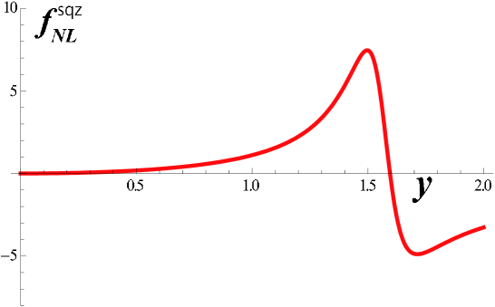
Figure 2: The same as Fig. 1 but for $f^{sqz}_{NL}(k)$.

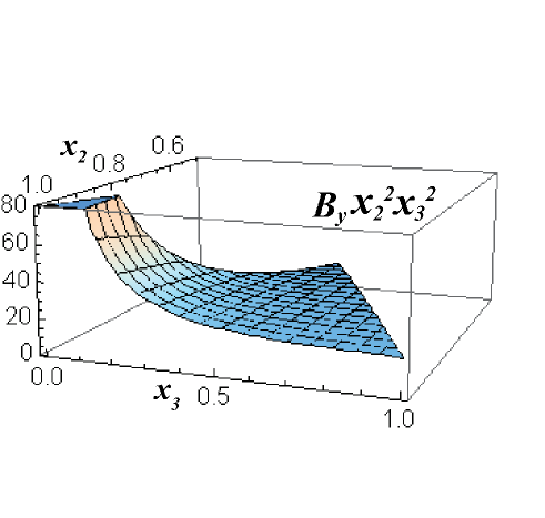
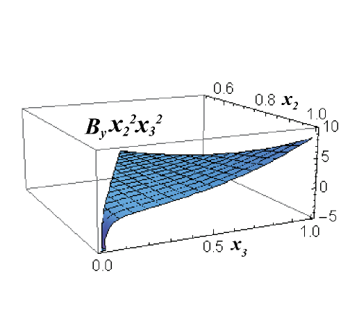
Figure 3: ${\cal B}_{y}(1,x_{2},x_{3})x_{2}^{2}x_{3}^{2}$ as a function of $x_{2}$ and $x_{3}$ for $y=1$ (left) and $y=10$ (right). The bispectrum has a peak at the squeezed shape ($x_{2}=1$, $x_{3}=0$) for $y=1$, while it has a peak at the equilateral shape ($x_{2}=x_{3}=1$) and a negative peak at the squeezed shape for $y=10$.

To see the shape dependence of $B_{\zeta}$, it is convenient to define a dimensionless function,

$${\cal B}_{y}(x_{1},x_{2},x_{3}) \equiv \frac{5k_{0}^{6}}{8\pi^{4}({\cal P}^{(0)}_{{\cal R}})^{2}T^{3}}B_{\zeta}(k_{0}yx_{1}/\sqrt{T},k_{0}yx_{2}/\sqrt{T},k_{0}yx_{3}/\sqrt{T})$$ (171)

$$\approx \frac{1}{y^{4}x_{1}^{3}x_{2}^{3}x_{3}^{3}}\left[\left(1-\frac{2}{5}y^{2}x_{1}^{2}\right)\left(1-\frac{2}{5}y^{2}x_{2}^{2}\right)\left[5(x_{1}^{2}+x_{2}^{2})-x_{3}^{2}\right]x_{3}^{3}+\mbox{cyclic}\right]\,,$$

and identify the dimensionless variables as

$$y=\sqrt{T}k_{1}/k_{0}\,,\quad x_{1}=1\,,\quad x_{2}=k_{2}/k_{1}\,,\quad x_{3}=k_{3}/k_{1}\,,$$ (172)

so that

$$B_{\zeta}(k_{1},k_{2},k_{3})=\frac{8\pi^{4}({\cal P}^{(0)}_{{\cal R}})^{2}T^{3}}{5k_{0}^{6}}{\cal B}_{y}(1,x_{2},x_{3}).$$ (173)

Without loss of generality, we can restrict our attention to the region $1-x_{2}<x_{3}<x_{2}<1$. We plot ${\cal B}_{y}(1,x_{2},x_{3})x_{2}^{2}x_{3}^{2}$ for $y=1$ and $y=10$ as a function of $x_{2}$ and $x_{3}$ in Fig. 3. For small $y$, we see that the bispectrum has a peak at the squeezed shape. On the other hand, for larger $y$, there is a positive peak at the equilateral shape as well as a negative peak at the squeezed shape.

VII Summary and discussion

We have developed a theory of nonlinear cosmological perturbations on superhorizon scales for a single scalar field with a general kinetic term and a general form of the potential to second-order in the spatial gradient expansion. The solution to this order is necessary to evaluate correctly the final amplitude of the curvature perturbation for models of inflation with a temporary violation of the slow-roll condition. We have employed the ADM formalism and obtained the general solution for full nonlinear curvature perturbations valid up through second-order in the gradient expansion. We have introduced a reasonable variable that represents the nonlinear curvature perturbation on comoving slices ${\cal R}_{c}^{\rm NL}$, which reduces to the comoving curvature perturbation ${\cal R}_{c}^{\rm Lin}$ in the linear limit. Then we have found that ${\cal R}_{c}^{\rm NL}$ satisfies a nonlinear second-order differential equation, (82), as a natural extension of the linear second-order differential equation.

Then we have formulated the matching of the nonlinear solution to a perturbative solution at $n$-th-order, ${\cal R}_{c}^{\rm pert}$, on superhorizon scales, and obtained a formula for the final value of the nonlinear curvature perturbation expressed in terms of ${\cal R}_{c}^{\rm pert}$ and its time derivative at the time of matching. Since the evolution of superhorizon curvature perturbations is genuinely due to the $O(\epsilon^{2})$ effect, our formulation can be used to calculate the primordial non-Gaussianity beyond the $\delta N$ formalism which is equivalent to leading order in the gradient expansion.

Then we have considered the case when the linear approximation is valid up to the time of horizon crossing for wavenumbers of physical interest. In this case, we have developed a method to determine quantities corresponding to ${\cal R}_{c}^{\rm pert}$ and its time derivative at the matching time in terms of the linear solution.

As an example of such a case, we have investigated Starobinsky’s model Starobinsky:1992ts in which there is a temporary non-slow-roll stage during inflation due to a sudden change of the potential slope. We have found that non-Gaussianity can become large if the parameter $T\approx{A_{+}/A_{-}}$, which characterises the ratio of the slope before and after the transition, is large. For $T\gg 1$, we have found that the non-Gaussianity parameter for the bispectrum $f_{NL}({k}_{1},{k}_{2},{k}_{3})$ is peaked at the wavenumbers forming an equilateral triangle, $k=k_{1}=k_{2}=k_{3}$, denoted by $f_{NL}^{eql}(k)$. It is found to be positive and takes the maximum value $f_{NL}^{eql}(k)\simeq 2T$ at $y=\sqrt{T}k/k_{0}\simeq 1.5$ where $k_{0}$ is the comoving wavenumber that crosses the horizon at the time when the potential slope changes. This implies that, even for a relatively small $T$, say for $T=10$, it is possible to generate a fairly large non-Gaussianity $f_{NL}\sim 20$ at wavenumber $k\simeq 0.5k_{0}$.

Our formalism can be applied to many other interesting circumstances in which the slow-roll condition is temporarily violated. To mention a couple of examples, a non-slow-roll stage appears in a double inflation model Saito:2008em or in a specific case of DBI inflation Jain:2007au . It is of interest to investigate the non-Gaussianity in these models by applying our formalism.

It is also of interest to investigate the case when there is a step in the inflaton potential instead of a change in the slope, which was proposed to explain the ‘features’ in the cosmic microwave background anisotropy Chen:2006xjb ; Joy:2008qd . The case of time-varying sound speed for models with non-canonical kinetic terms Khoury:2008wj may also deserve future study, since a rapid temporal variation of the sound velocity violates a certain type of the slow-roll condition.

Finally, here we have focused on the case of a single scalar field. An immediate issue is to extend the present formalism to the case of a multi-component scalar field. We plan to work on this and hope to report the result in the near future.

Appendix A Useful formulas from background equations

In this Appendix, we derive some useful formulas that are used in Sec. III.4 to modify the apparent forms of the functions $f_{K}(t)$ and $f_{C}(t)$ defined in (45) and (46).

Using the background equations,

$$\dot{H}=-{\kappa^{2}\over 2}(\rho+P)\,,\quad\frac{d}{dt}\left({1\over\rho+P}\right)={3(1+c_{s}^{2})H\over\rho+P}-{\rho\Gamma\dot{\phi}\over(\rho+P)^{2}}\,,$$ (174)

we obtain a useful formula by integrating the time derivative of $(a/H)$,

$$\int_{t_{*}}^{t}a(t^{\prime})dt^{\prime}=\biggl{[}{a\over H}\biggr{]}^{t}_{t_{*}}-{\kappa^{2}\over 2}\int_{t_{*}}^{t}{a(\rho+P)\over H^{2}}dt^{\prime}\,.$$ (175)

Then using the quantity $z$ defined in (72),

$$z={{a\over H}\left(\rho+P\over c_{s}^{2}\right)^{1\over 2}}\,,$$ (176)

the above can be further transformed to

$${d\over dt}{\left({1\over a(t)}\int_{t_{*}}^{t}a(t^{\prime})dt^{\prime}\right)}={\kappa^{2}H\over 2a}\int_{\eta_{*}}^{\eta}z^{2}c_{s}^{2}(\eta^{\prime})d\eta^{\prime}+{a_{*}H(t)\over a(t)H_{*}}\,,$$ (177)

where the subscript $*$ indicates that the quantity is estimated at $t=t_{*}$ (or $\eta=\eta_{*}$). With the help of (174) and (177), we obtain

$$\int_{t_{*}}^{t}{H\rho\Gamma\dot{\phi}\over 2(\rho+P)^{2}a^{3}}\,(t^{\prime})dt^{\prime}\int_{t_{*}}^{t^{\prime}}a(t^{\prime\prime})dt^{\prime\prime} = -{H\over 2(\rho+P)a^{3}}\int_{t_{*}}^{t}a(t^{\prime})dt^{\prime}+\int_{t_{*}}^{t}{dt^{\prime}\over(\rho+P)}\,\partial_{t^{\prime}}\left({H(t^{\prime})\int_{t_{*}}^{t^{\prime}}a(t^{\prime\prime})dt^{\prime\prime}\over 2a^{3}(t^{\prime})}\right)$$ (178)

$$+\int_{t_{*}}^{t}{3(1+c_{s}^{2})H^{2}\over 2(\rho+P)a^{3}}(t^{\prime})dt^{\prime}\int_{t_{*}}^{t^{\prime}}a(t^{\prime\prime})dt^{\prime\prime},$$

where the second term in the right hand side of the above equation can be rewritten as

$$\int_{t_{*}}^{t}{dt^{\prime}\over(\rho+P)}\,\partial_{t^{\prime}}\left({H\over 2a^{2}}\,{\int_{t_{*}}^{t^{\prime}}a(t^{\prime\prime})dt^{\prime\prime}\over a(t^{\prime})}\right) = -{\kappa^{2}\over 4}\int_{t_{*}}^{t}{dt^{\prime}\over a^{3}(t^{\prime})}\int_{t_{*}}^{t^{\prime}}a(t^{\prime\prime})dt^{\prime\prime}-\int_{t_{*}}^{t}{H^{2}\over(\rho+P)a^{3}}(t^{\prime})dt^{\prime}\int_{t_{*}}^{t^{\prime}}a(t^{\prime\prime})dt^{\prime\prime}$$ (179)

$$+{\kappa^{2}\over 4}\int_{\eta_{*}}^{\eta}{d\eta^{\prime}\over z^{2}c_{s}^{2}(\eta^{\prime})}\int_{\eta_{*}}^{\eta^{\prime}}z^{2}c_{s}^{2}(\eta^{\prime\prime})d\eta^{\prime\prime}+\int_{\eta_{*}}^{\eta}{d\eta^{\prime}\over 2z^{2}c_{s}^{2}(\eta^{\prime})}{a_{*}\over H_{*}},$$

and similarly, we obtain

$$\int_{t_{*}}^{t}{H\rho\Gamma\dot{\phi}\over 2(\rho+P)^{2}a^{3}}(t^{\prime})dt^{\prime}=-{H\over 2(\rho+P)a^{3}}\bigg{|}^{t}_{t_{*}}-{\kappa^{2}\over 4}\int_{t_{*}}^{t}{dt^{\prime}\over a^{3}(t^{\prime})}+{3\over 2}\int_{t_{*}}^{t}{d\eta^{\prime}\over z^{2}(\eta^{\prime})}\,.$$ (180)

Appendix B $t_{*}$-independence in Linear theory

In the linear theory the curvature perturbation ${\cal R}^{\rm Lin}_{c,\bm{k}}(\eta)$ in the Fourier space satisfies

$${{\cal R}^{\rm Lin}_{c,\bm{k}}}^{\prime\prime}+2\frac{z^{\prime}}{z}{{\cal R}^{\rm Lin}_{c,\bm{k}}}^{\prime}+c_{s}^{2}k^{2}{\cal R}^{\rm Lin}_{c,\bm{k}}=0,$$ (181)

and is related to $u^{(0)}_{\bm{k}}$ up to $O(k^{2})$ as

$${\cal R}^{\rm Lin}_{c,\bm{k}}(\eta) = \left[\alpha^{\rm Lin}_{\bm{k}}+(1-\alpha^{\rm Lin}_{\bm{k}})\frac{D(\eta)}{D_{*}}-\left(\frac{F_{*}}{D_{*}}D(\eta)-F(\eta)\right)k^{2}+O(k^{4})\right]u^{(0)}_{\bm{k}}$$ (182)

$$= \left[1-\beta^{\rm Lin}_{\bm{k}}\left(1-\frac{D(\eta)}{D_{*}}\right)-\left(\frac{F_{*}}{D_{*}}D(\eta)-F(\eta)\right)k^{2}+O(k^{4})\right]u^{(0)}_{\bm{k}},$$

where

$$D(\eta)=3{\cal H}_{*}\int_{\eta}^{0}\frac{z^{2}(\eta_{*})}{z^{2}(\eta^{\prime})}d\eta^{\prime},\quad F(\eta)=\int_{\eta}^{0}\frac{d\eta^{\prime}}{z^{2}(\eta^{\prime})}\int_{\eta_{*}}^{\eta^{\prime}}z^{2}(\eta^{\prime\prime})c_{s}^{2}(\eta^{\prime\prime})d\eta^{\prime\prime},$$ (183)

$$D_{*}=D(\eta_{*}),\quad F_{*}=F(\eta_{*}),$$ (184)

and

$$\beta^{\rm Lin}_{\bm{k}}=1-\alpha^{\rm Lin}_{\bm{k}}=-\frac{D_{*}}{3{\cal H}_{*}}\left.\frac{{{\cal R}^{\rm Lin}_{c,\bm{k}}}^{\prime}}{{\cal R}^{\rm Lin}_{c,\bm{k}}}\right|_{\eta=\eta_{*}}+k^{2}F_{*}.$$ (185)

In our paper we have assumed that

$$\beta^{\rm Lin}_{\bm{k}}=O(k^{2}).$$ (186)

By inverting the relation (182) and setting $\eta=\eta_{k}$, $u^{(0)}_{\bm{k}}$ is expressed as

$$u^{(0)}_{\bm{k}}=\left[1+\beta^{\rm Lin}_{\bm{k}}\left(1-\frac{D_{k}}{D_{*}}\right)+\left(\frac{F_{*}}{D_{*}}D_{k}-F_{k}\right)k^{2}+O(k^{4})\right]{\cal R}^{\rm Lin}_{c,\bm{k}}(\eta_{k}),$$ (187)

where

$$D_{k}=D(\eta_{k}),\quad F_{k}=F(\eta_{k}).$$ (188)

Hence,

$$\alpha^{\rm Lin}_{\bm{k}}u^{(0)}_{\bm{k}} = \left[1-\frac{D_{k}}{D_{*}}\beta^{\rm Lin}_{\bm{k}}+\left(\frac{F_{*}}{D_{*}}D_{k}-F_{k}\right)k^{2}+O(k^{4})\right]{\cal R}^{\rm Lin}_{c,\bm{k}}(\eta_{k})$$ (189)

$$= \left[1+\frac{D_{k}}{3{\cal H}_{*}}\left.\frac{{{\cal R}^{\rm Lin}_{c,\bm{k}}}^{\prime}}{{\cal R}^{\rm Lin}_{c,\bm{k}}}\right|_{\eta=\eta_{*}}-k^{2}F_{k}+O(k^{4})\right]{\cal R}^{\rm Lin}_{c,\bm{k}}(\eta_{k})$$

$$= \left\{1-k^{2}\tilde{F}_{k}+\left[k^{2}\int_{\eta_{k}}^{\eta_{*}}z^{2}(\eta^{\prime\prime})c_{s}^{2}(\eta^{\prime\prime})d\eta^{\prime\prime}+\left.\frac{z^{2}{{\cal R}^{\rm Lin}_{c,\bm{k}}}^{\prime}}{{\cal R}^{\rm Lin}_{c,\bm{k}}}\right|_{\eta=\eta_{*}}\right]\int_{\eta_{k}}^{0}\frac{d\eta^{\prime}}{z^{2}(\eta^{\prime})}+O(k^{4})\right\}{\cal R}^{Lin}_{c,\bm{k}}(\eta_{k}),$$

where

$$\tilde{F}_{k}=\int_{\eta_{k}}^{0}\frac{d\eta^{\prime}}{z^{2}(\eta^{\prime})}\int_{\eta_{k}}^{\eta^{\prime}}z^{2}(\eta^{\prime\prime})c_{s}^{2}(\eta^{\prime\prime})d\eta^{\prime\prime}.$$ (190)

By using (181), it is easy to show that

$$\left(\frac{z^{2}{{\cal R}^{\rm Lin}_{c,\bm{k}}}^{\prime}}{{\cal R}^{\rm Lin}_{c,\bm{k}}}\right)^{\prime}=-k^{2}z^{2}c_{s}^{2}-\left(\frac{z{{\cal R}^{\rm Lin}_{c,\bm{k}}}^{\prime}}{{\cal R}^{\rm Lin}_{c,\bm{k}}}\right)^{2}=-k^{2}z^{2}c_{s}^{2}+O(k^{4}).$$ (191)

This implies that

$$k^{2}\int_{\eta_{k}}^{\eta_{*}}z^{2}(\eta^{\prime\prime})c_{s}^{2}(\eta^{\prime\prime})d\eta^{\prime\prime}=-\left.\frac{z^{2}{{\cal R}^{\rm Lin}_{c,\bm{k}}}^{\prime}}{{\cal R}^{\rm Lin}_{c,\bm{k}}}\right|_{\eta=\eta_{*}}+\left.\frac{z^{2}{{\cal R}^{Lin}_{c,\bm{k}}}^{\prime}}{{\cal R}^{\rm Lin}_{c,\bm{k}}}\right|_{\eta=\eta_{k}}+O(k^{4}).$$ (192)

Therefore, we obtain

$$\alpha^{\rm Lin}_{\bm{k}}u^{(0)}_{\bm{k}}=\tilde{\alpha}^{\rm Lin}_{\bm{k}}{\cal R}^{\rm Lin}_{c,\bm{k}}(\eta_{k})+O(k^{4}),$$ (193)

where

$$\tilde{\alpha}^{\rm Lin}_{\bm{k}}=1-k^{2}\tilde{F}_{k}+\int_{\eta_{k}}^{0}\frac{d\eta^{\prime}}{z^{2}(\eta^{\prime})}\times\left.\frac{z^{2}{{\cal R}^{\rm Lin}_{c,\bm{k}}}^{\prime}}{{\cal R}^{\rm Lin}_{c,\bm{k}}}\right|_{\eta=\eta_{k}},$$ (194)

and $\tilde{F}_{k}$ is given by (190). This explicitly shows that $\alpha^{\rm Lin}_{\bm{k}}u^{(0)}_{\bm{k}}$ is independent of $\eta_{*}$ up through $O(k^{2})$.

References

-
(1)
E. Komatsu et al. [WMAP Collaboration],
Astrophys. J. Suppl. 148, 119 (2003)
[arXiv:astro-ph/0302223].
D. N. Spergel et al. [WMAP Collaboration], Astrophys. J. Suppl. 170, 377 (2007) [arXiv:astro-ph/0603449]. - (2) E. Komatsu et al., arXiv:1001.4538 [astro-ph.CO].
- (3) N. Bartolo, E. Komatsu, S. Matarrese and A. Riotto, Phys. Rept. 402, 103 (2004) [arXiv:astro-ph/0406398].
- (4) E. Komatsu and D. N. Spergel, Phys. Rev. D 63, 063002 (2001) [arXiv:astro-ph/0005036].
- (5) [Planck Collaboration], arXiv:astro-ph/0604069.
- (6) D. Seery and J. E. Lidsey, JCAP 0506, 003 (2005) [arXiv:astro-ph/0503692].
-
(7)
G. I. Rigopoulos and E. P. S. Shellard,
Phys. Rev. D 68, 123518 (2003)
[arXiv:astro-ph/0306620].
G. I. Rigopoulos and E. P. S. Shellard, JCAP 0510, 006 (2005) [arXiv:astro-ph/0405185]. -
(8)
D. H. Lyth and Y. Rodriguez,
Phys. Rev. Lett. 95, 121302 (2005)
[arXiv:astro-ph/0504045].
D. H. Lyth and Y. Rodriguez, Phys. Rev. D 71, 123508 (2005) [arXiv:astro-ph/0502578]. - (9) D. Seery and J. E. Lidsey, JCAP 0509, 011 (2005) [arXiv:astro-ph/0506056].
- (10) M. Sasaki and T. Tanaka, Prog. Theor. Phys. 99, 763 (1998) [arXiv:gr-qc/9801017].
- (11) D. H. Lyth, K. A. Malik and M. Sasaki, JCAP 0505, 004 (2005) [arXiv:astro-ph/0411220].
- (12) D. Langlois and F. Vernizzi, JCAP 0702, 017 (2007) [arXiv:astro-ph/0610064].
- (13) J. M. Maldacena, JHEP 0305, 013 (2003) [arXiv:astro-ph/0210603].
-
(14)
S. Yokoyama, T. Suyama and T. Tanaka,
JCAP 0707, 013 (2007)
[arXiv:0705.3178 [astro-ph]].
S. Yokoyama, T. Suyama and T. Tanaka, Phys. Rev. D 77, 083511 (2008) [arXiv:0711.2920 [astro-ph]]. -
(15)
C. T. Byrnes, K. Y. Choi and L. M. H. Hall,
JCAP 0810, 008 (2008)
[arXiv:0807.1101 [astro-ph]].
C. T. Byrnes and G. Tasinato, JCAP 0908, 016 (2009) [arXiv:0906.0767 [astro-ph.CO]]. - (16) T. Suyama and M. Yamaguchi, Phys. Rev. D 77, 023505 (2008) [arXiv:0709.2545 [astro-ph]].
-
(17)
M. Sasaki,
Prog. Theor. Phys. 120, 159 (2008)
[arXiv:0805.0974 [astro-ph]].
A. Naruko and M. Sasaki, Prog. Theor. Phys. 121, 193 (2009) [arXiv:0807.0180 [astro-ph]]. - (18) K. A. Malik and D. H. Lyth, JCAP 0609, 008 (2006) [arXiv:astro-ph/0604387].
- (19) M. Sasaki, J. Valiviita and D. Wands, Phys. Rev. D 74, 103003 (2006) [arXiv:astro-ph/0607627].
- (20) M. Alishahiha, E. Silverstein and D. Tong, Phys. Rev. D 70, 123505 (2004) [arXiv:hep-th/0404084].
- (21) X. Chen, M. x. Huang, S. Kachru and G. Shiu, JCAP 0701, 002 (2007) [arXiv:hep-th/0605045].
-
(22)
X. Chen, R. Easther and E. A. Lim,
JCAP 0706, 023 (2007)
[arXiv:astro-ph/0611645].
X. Chen, R. Easther and E. A. Lim, JCAP 0804, 010 (2008) [arXiv:0801.3295 [astro-ph]]. - (23) D. Wands, K. A. Malik, D. H. Lyth and A. R. Liddle, Phys. Rev. D 62, 043527 (2000) [arXiv:astro-ph/0003278].
- (24) M. Sasaki and E. D. Stewart, Prog. Theor. Phys. 95, 71 (1996) [arXiv:astro-ph/9507001].
- (25) A. A. Starobinsky, JETP Lett. 42, 152 (1985) [Pisma Zh. Eksp. Teor. Fiz. 42, 124 (1985)].
- (26) L. Senatore, K. M. Smith and M. Zaldarriaga, JCAP 1001, 028 (2010) [arXiv:0905.3746 [astro-ph.CO]].
- (27) Y. Nambu and A. Taruya, Class. Quant. Grav. 13, 705 (1996) [arXiv:astro-ph/9411013].
- (28) D. S. Salopek and J. R. Bond, Phys. Rev. D 42, 3936 (1990).
- (29) H. Kodama and T. Hamazaki, Phys. Rev. D 57, 7177 (1998) [arXiv:gr-qc/9712045].
- (30) S. M. Leach, M. Sasaki, D. Wands and A. R. Liddle, Phys. Rev. D 64, 023512 (2001) [arXiv:astro-ph/0101406].
- (31) O. Seto, J. Yokoyama and H. Kodama, Phys. Rev. D 61, 103504 (2000) [arXiv:astro-ph/9911119].
-
(32)
R. K. Jain, P. Chingangbam and L. Sriramkumar,
JCAP 0710, 003 (2007)
[arXiv:astro-ph/0703762].
R. K. Jain, P. Chingangbam, L. Sriramkumar and T. Souradeep, arXiv:0904.2518 [astro-ph.CO]. - (33) Y. Tanaka and M. Sasaki, Prog. Theor. Phys. 117, 633 (2007) [arXiv:gr-qc/0612191].
- (34) Y. Tanaka and M. Sasaki, Prog. Theor. Phys. 118, 455 (2007) [arXiv:0706.0678 [gr-qc]].
- (35) Y. Takamizu and S. Mukohyama, JCAP 0901, 013 (2009) [arXiv:0810.0746 [gr-qc]].
- (36) J. Garriga and V. F. Mukhanov, Phys. Lett. B 458, 219 (1999) [arXiv:hep-th/9904176].
- (37) T. Hamazaki, Phys. Rev. D 78, 103513 (2008) [arXiv:0811.2366 [astro-ph]].
- (38) H. Kodama and M. Sasaki, Prog. Theor. Phys. Suppl. 78 (1984) 1.
- (39) V. F. Mukhanov, H. A. Feldman and R. H. Brandenberger, Phys. Rept. 215, 203 (1992).
- (40) S. M. Leach and A. R. Liddle, Phys. Rev. D 63, 043508 (2001) [arXiv:astro-ph/0010082].
- (41) R. Saito, J. Yokoyama and R. Nagata, JCAP 0806, 024 (2008) [arXiv:0804.3470 [astro-ph]].
- (42) A. A. Starobinsky, JETP Lett. 55 (1992) 489 [Pisma Zh. Eksp. Teor. Fiz. 55 (1992) 477].
- (43) M. Joy, A. Shafieloo, V. Sahni and A. A. Starobinsky, JCAP 0906, 028 (2009) [arXiv:0807.3334 [astro-ph]].
- (44) J. Khoury and F. Piazza, JCAP 0907, 026 (2009) [arXiv:0811.3633 [hep-th]].