Abstract

It is well-known that the Ricci flow of a closed 3-manifold containing an essential minimal 2-sphere will fail to exist after a finite time. Conversely, the Ricci flow of a complete, rotationally symmetric, asymptotically flat manifold containing no minimal spheres is immortal. We discuss an intermediate case, that of a complete, noncompact manifold with essential minimal hypersphere. For 3-manifolds, if the scalar curvature vanishes on asymptotic ends and is bounded below initially by a negative constant that depends on the area of the minimal sphere, we show that a singularity develops in finite time. In particular, this result applies to asymptotically flat manifolds, which are a boundary case with respect to the neckpinch theorem of M Simon. We provide numerical evolutions to explore the case where the initial scalar curvature is less than the bound.

1 Introduction

A Ricci flow on a manifold $M$ is a family of Riemannian metrics $g_{ij}(t;x)$, $x\in M$, $t\in I\subseteq{\mathbb{R}}$ the family parameter, and $I$ a connected interval, satisfying

$$\frac{\partial g_{ij}}{\partial t}=-2R_{ij}\ ,$$ (1.1)

where $R_{ij}$ is the Ricci tensor of $g_{ij}(t,x)$. It is usually more convenient to study the Hamilton-DeTurck flow (or Ricci-DeTurck flow)

$$\frac{\partial g_{ij}}{\partial t}=-2R_{ij}+\pounds_{X}g_{ij}\ .$$ (1.2)

If $g$ solves (1.2), then the pullback $\psi_{t}^{*}g$ solves (1.1) ([2], p 80), where $\psi_{t}$ is a family of time-dependent diffeomorphisms generated by the vector field $X$. From (1.2), the scalar curvature $R$ of $g_{ij}(t)$ evolves according to

$$\frac{\partial R}{\partial t}=\Delta R+\nabla_{X}R+2R_{ij}R^{ij}\ ,$$ (1.3)

where $\Delta:=g^{ij}\nabla_{i}\nabla_{j}$ is the ($t$-dependent) Laplacian.

Ricci flow of asymptotically flat manifolds arises in several physical and mathematical contexts, ranging from the physics of closed string tachyon condensation [8] to existence problems for static Einstein metrics [7]. It is known that asymptotically flat initial data remain asymptotically flat and smooth when evolved by Ricci flow for some time interval $[0,T)$ [4, 13]. For complete, rotationally symmetric initial data with no minimal sphere present (corresponding in static general relativity to the absence of black hole horizons), it has been shown that the flow exists for all future time and converges to flat space [13].

Then the question arises as to what happens when complete, rotationally symmetric initial data containing a minimal sphere are evolved. There are two cases, depending on whether the minimal sphere is topologically essential (representing a nontrivial class in $\pi_{2}(M)$) or, as will be the case for data on ${\mathbb{R}}^{n}$, inessential. Of these, the essential case is the easier one to study, and is the subject of the present paper.

It is well-known that a closed 3-manifold admitting an essential minimal 2-sphere, when evolved under the Ricci flow, will develop a singularity within finite time. Depending on the initial configuration, the singularity may be localized at or near the minimal sphere, or may be global in the sense that the manifold collapses everywhere at that time. It is expected that this result carries over to the noncompact case. Somewhat to the contrary though, asymptotically flat initial data are critical data with respect to the pinching theorem of M Simon [14]. That is, Simon proves that warped products of a line with a positively curved closed manifold will evolve to form a neckpinch singularity in finite time, provided the initial data obey certain asymptotic conditions at the ends of the line, including a condition on asymptotic growth of the area of the closed manifold factor. Simon’s growth condition is written as a strict (i.e., open) inequality which is not satisfied by asymptotically flat manifolds, but such manifolds would lie in the closure. This suggests that such data may exhibit interesting evolutions, including perhaps critical phenomena of the sort observed in certain numerical evolutions in general relativity in a scenario sometimes called “critical collapse” [1].

Garfinkle and Isenberg [5] studied numerical Hamilton-DeTurck flow of a 3-sphere with “corsetted” initial metric, admitting an inessential minimal 2-sphere (the “waist”). For tight corsetting, meaning that the waist has very small area relative to the $2/3^{\rm rds}$-power of the volume of the 3-sphere, the waist “pinches off” (a local singularity forms there), whereas for more gentle corsetting, the entire sphere shrinks to a point before a local singularity can form. The critical solution separating these two alternatives is a degenerate neckpinch singularity modelled by the Bryant soliton [6].

The Garfinkle-Isenberg result shows that initial data for the Ricci flow with an inessential minimal sphere divides into two disjoint sets whose common boundary consists of points whose evolutions exhibit critical behaviour.

Husain and Seahra [10] then considered a numerical Hamilton-DeTurck flow of a sequence of initial metrics, each rotationally symmetric and reflection symmetric through an essential minimal 2-sphere, sometimes referred to as the “throat” or “bridge”. Evolution occurred on a bounded region, with boundary conditions imposed. Two alternatives were again found; for some initial data, the throat pinched off while, for other data, the throat expanded to infinity.

We study a related question. Consider simply connected, noncompact, complete manifolds with rotational symmetry. These are ${\mathbb{R}}^{n}$, ${\mathbb{R}}\times S^{n-1}$, and certain quotients thereof. As ${\mathbb{R}}^{n}$ has no essential minimal sphere, consider ${\mathbb{R}}\times S^{n-1}$, and endow it with an ${\rm SO}(n)$-symmetric metric such that there is a minimal hypersphere located at, say, $r=0$ and an isometry corresponding to reflection in that hypersphere. One such metric is the $t=0$ slice of the $(n+1)$-dimensional Schwarzschild-Tangherlini metric. One can then identify points under the action ${\mathbb{R}}\times S^{n-1}\ni(r,p)\mapsto(-r,-p)$, where $p\in S^{n-1}$ and $-p$ is the antipode of $p$. This produces a smooth metric on ${\mathbb{R}}\times{\mathbb{R}}{\mathbb{P}}^{n-1}\cong{\mathbb{R}}{\mathbb{P}}^{n}\setminus\{{\rm pt}\}$. For $n=3$, this model is known in gravitational physics as the ${\mathbb{R}}{\mathbb{P}}^{3}$ geon. We pose and will answer the question, “What is the Ricci flow evolution of the ${\mathbb{R}}{\mathbb{P}}^{3}$ geon?”

In section 2, we adapt a standard Ricci flow argument from the setting of closed manifolds to that of asymptotically flat manifolds. This forms the basis for what follows, and shows that essential 2-spheres in asymptotically flat 3-manifolds collapse whenever the initial scalar curvature is bounded below by a nonpositive constant that can depend on the initial area of the minimal sphere. The result is valid for arbitrary Hamilton-DeTurck flow, including Ricci flow. As the covering space of the ${\mathbb{R}}{\mathbb{P}}^{3}$ geon obeys this bound, this suffices to answer the question just posed.

This raises the possibility that, by choosing initial data for which the lower bound on initial scalar curvature is violated (e.g., by choosing a different initial metric on the geon manifold, with the same isometries), interesting dynamics might arise, such as observed in the studies cited above [5, 6, 10]. It also raises the question of the precise comparison, if any, of this result to the numerical work of [10], who found that for certain initial data with scalar curvature well above our lower bound, their numerical Hamilton-DeTurck evolution did not lead to collapse.

To understand these issues, we perform our own numerical simulations. In section 3, we lay the groundwork. We first discuss Hamilton-DeTurck flow with the “DeTurck trick” formulation which we use for our numerical evolutions in Section 4 (and which [5] used). For comparison purposes, we then discuss the normal coordinate Hamilton-DeTurck formulation used in [10].

Section 4 contains our numerical results. We use the same form of initial data as Husain and Seahra [10] and, for practical purposes, we also now restrict our evolution to a bounded manifold, but we use different evolution equations and different boundary conditions at the boundary at large $r$. Our numerical evolutions always exhibit collapse of the throat. Section 5 contains a brief discussion of the numerical evolution.

Our convention for the curvature tensor $R^{a}{}_{bcd}$ is that used in [9] and equals the quantity denoted by $R_{cdb}{}^{a}$ in [2]. We write $R_{abcd}:=g_{ae}R^{e}{}_{bcd}$. We denote the Laplacian by $\Delta:=g^{ab}\nabla_{a}\nabla_{b}$. For a definition of asymptotic flatness, see [13].

2 Time derivative of the area of a minimal sphere

2.1 The maximum principle for scalar curvature

For Ricci flow on compact manifolds, it is standard that positive scalar curvature is associated to contraction and concentration of curvature under the Ricci flow. In this subsection is that scalar curvature, we recall that this is also true for complete manifolds with vanishing scalar curvature at infinity.

Proposition 2.1. Assume that (1.3) has a solution on some time interval $[0,T]$, $T>0$, on a complete manifold $M$ with one or more asymptotic ends, and assume that $R(t,x)\to 0$ as $x\to\infty$ (that is, as the point $x$ tends to an asymptotic end), for all $t\in[0,T]$. Let the scalar curvature $R_{0}(x)$ of the initial metric $g_{0}(x):=g(0,x)$ obey

$$\inf_{x\in{\cal M}}\left\{R_{0}(x)\right\}=:-a^{2}\ ,$$ (2.1)

for some $a\geq 0$. Then

$$R(t,x)\geq\frac{-a^{2}}{1+\frac{2a^{2}}{n}t}\ .$$ (2.2)

Remark 2.2. The existence assumption always holds for Ricci flow developing from asymptotically flat initial data ([13], [4]).

Proof. Equation (1.3) can be written as

$$\frac{\partial R}{\partial t}=\Delta R+\frac{2}{n}R^{2}+2\left|R_{ij}-\frac{1}{n}g_{ij}R\right|^{2}+\nabla_{X}R\ .$$ (2.3)

Exhaust $M$ by a sequence of closed, bounded sets $K_{i}$. An easy application of the maximum principle (e.g., [11]) to the $i^{\rm th}$ subset yields that the minimum of $R$ occurs on the parabolic boundary of $[0,T]\times K_{i}$. Now take $i\to\infty$ and use that $R(t,x)\to 0$ as $x\to\infty$ to deduce that the minimum must either be zero or must occur on the initial data. This proves that

$$R(t,x)\geq\inf_{x\in{\cal M}}\left\{R_{0}(x)\right\}=-a^{2},\ a\geq 0.$$ (2.4)

If $a=0$, this proves the theorem, so we now consider $a>0$, in which case the infimum is a minimum.

For $a>0$, let $Q:=-\frac{1}{a^{2}}\left(1+\frac{2a^{2}}{n}t\right)R$. Since $R=-a^{2}<0$ at its minimum, then $Q>0$ there. Hence the maximum of $Q$ is positive, and it then follows from the definition of $Q$ that, at the point where $Q$ achieves its maximum, $R$ is negative. As well, $Q(t,x)\to 0$ as $x\to\infty$.

Work on the intervalcompact set $[0,T]\times K_{i}$. From (2.3), we have

$$\frac{\partial Q}{\partial t}\leq\Delta Q+\nabla_{X}Q+\frac{2}{n}R\left(Q-1\right)\ .$$ (2.5)

Then from the maximum principle (and since $R<0$ where $Q$ achieves its maximum), either the maximum of $Q$ occurs on the parabolic boundary of $[0,T]\times K_{i}$ or $Q-1\leq 0$ at the maximum. If it occurs on the parabolic boundary, by taking $i\to\infty$ and using that $Q(t,x)\to 0$ as $x\to\infty$, we see that the maximum must occur on the initial boundary, where $Q(0,x)=-\frac{1}{a^{2}}R(0,x)\leq 1$. Hence, $Q(t,x)\leq 1$, and the result follows. ∎

Remark 2.3. Obviously, these results also hold on $[0,T]\times K$, $K\subset M$ a compact set with boundary $\partial K$, provided that $R(t,x)=0$ for $x\in\partial K$. But they do not hold if merely $R(t,x)\geq-const$ on $\partial K$, an observation which appears to be relevant in numerical studies (see section 3.2.2).

2.2 Evolution of hypersurfaces

In this subsection, we obtain the evolution equation for the area of a closed hypersurface $\Sigma$ in an $n$-manifold $({\cal M}^{n},g)$, defined (locally at least) by an expression of the form $F(x^{i})=0$, where $x^{i}$ are the coordinates held constant in the derivative $\frac{\partial}{\partial t}$ appearing in (1.2).

Let $n^{a}$ be a smooth unit vector field normal to $\Sigma$. Let $h_{ab}$ be the induced metric and let $H_{ab}$ be the extrinsic curvature of $\Sigma$, with trace $H$ (thus $H$ is the mean curvature, taken here to mean the sum rather than the average of the principal curvatures at a point). If ${\tilde{H}}_{ab}$ denotes the trace-free part of $H_{ab}$, then

$$H_{ab}={\tilde{H}}_{ab}+\frac{1}{n-1}h_{ab}H\ .$$ (2.6)

If ${\cal R}$ denotes the scalar curvature of the induced metric $h_{ab}$ on $\Sigma$, then

$$R-{\rm Ric}(n,n)=\frac{1}{2}\left[{\cal R}-\left(\frac{n-2}{n-1}\right)H^{2}+R+|{\tilde{H}}|^{2}\right]$$ (2.7)

by the Gauss equation. Finally, let the induced area element on $\Sigma$ be $d\mu$. From the Hamilton-DeTurck flow equation (1.2), the area $|\Sigma|:=\int_{\Sigma}d\mu$ of $\Sigma$ evolves as

$$\frac{d}{dt}|\Sigma| = \int_{\Sigma}\frac{\partial}{\partial t}d\mu=\frac{1}{2}\int_{\Sigma}h^{ij}\frac{\partial h_{ij}}{\partial t}d\mu=\frac{1}{2}\int_{\Sigma}h^{ij}\frac{\partial g_{ij}}{\partial t}d\mu$$ (2.8)

$$= -\int_{\Sigma}h^{ij}\left(R_{ij}-\nabla_{i}X_{j}\right)d\mu=-\int_{\Sigma}\left(R-R_{ij}n^{i}n^{j}-h^{ij}\nabla_{i}X_{j}\right)d\mu$$

$$= -\frac{1}{2}\int_{\Sigma}\left({\cal R}-\left(\frac{n-2}{n-1}\right)H^{2}+R+|{\tilde{H}}|^{2}-2Hn\cdot X\right)d\mu\ ,$$

using (2.7), the divergence theorem on $\Sigma$, and $H:=h^{ij}\nabla_{i}n_{j}$.

2.3 3-manifolds

Now fix the dimension to be $n=3$. Then we have $\int_{\Sigma}{\cal R}d\mu=4\pi\chi(\Sigma)$, where $\chi(\Sigma)$ is the Euler characteristic of $\Sigma$. Then

$$\frac{d}{dt}|\Sigma|=-2\pi\chi(\Sigma)+W(\Sigma)-\frac{1}{2}\int_{\Sigma}\left(R+|{\tilde{H}}|^{2}\right)d\mu+\int_{\Sigma}Hn\cdot Xd\mu\ ,$$ (2.9)

where $W(\Sigma):=\frac{1}{4}\int_{\Sigma}H^{2}d\mu$ is the Willmore energy [15] of $\Sigma$. Using Proposition 2.1, (2.9) becomes

$$\frac{d}{dt}|\Sigma|\leq-2\pi\chi(\Sigma)+W(\Sigma)+\frac{3a^{2}|\Sigma|}{6+4t}+\int_{\Sigma}Hn\cdot Xd\mu\ .$$ (2.10)

The tightest bound occurs in the case of a minimal 2-sphere. Then $H|_{\Sigma}$ and the Willmore energy vanish and $\chi(S^{2})=2$ so

$$\frac{d}{dt}|\Sigma|\leq-4\pi+\frac{3a^{2}}{6+4t}|\Sigma|\ .$$ (2.11)

We note that the initial time derivative of $|\Sigma|$ will be negative whenever

$$a^{2}<\frac{8\pi}{|\Sigma|_{0}}\ ,$$ (2.12)

where $|\Sigma|_{0}$ denotes the initial area of $\Sigma$. Even when not initially negative, the derivative can turn negative and remain so thereafter.

Now we can regard the left-hand side of (2.11) as the forward difference quotient of the functional whose value is the area of the smallest essential minimal surface present at $t$. Then (see Lemma 2.22 of [12]) an upper barrier for the area of the smallest minimal surface at any $t\geq 0$ is provided by the function $\Psi(t)$ that solves the initial value problem

$$\frac{d\Psi}{dt}-\frac{3a^{2}\Psi}{6+4t} = -4\pi\ ,$$ (2.13)

$$\Psi(0)=|\Sigma|_{0}\ .$$

The solution is

$$\Psi(t)=\begin{cases}\frac{24\pi}{3a^{2}-4}(1+\frac{2}{3}t)+\left(|\Sigma|_{0}-\frac{24\pi}{3a^{2}-4}\right)\left(1+\frac{2}{3}t\right)^{3a^{2}/4}&\text{for $a^{2}\neq 4/3$,}\\ (1+\frac{2}{3}t)\left[|\Sigma|_{0}-6\pi\log\left(1+\frac{2}{3}t\right)\right]&\text{for $a^{2}=4/3$.}\end{cases}$$ (2.14)

Proposition 2.4. Say that the conditions of Proposition 2.1 hold and that $(M,g_{0})$ contains a minimal sphere of area $4\pi\delta$ for some $\delta>0$. Let $3a^{2}-4<6/\delta$. Then the flow fails to exist in finite time.

Proof. We must show that if the flow lasts long enough, the minimal sphere collapses. If $a^{2}=4/3$, this is immediate from the second line of (2.14), since $\Psi$ has a zero at some $t>0$. Otherwise, let $\gamma:=3a^{2}-4\neq 0$. The top line of (2.14) becomes

$$\Psi(t)=4\pi\left(1+\frac{2}{3}t\right)\left[\frac{6}{\gamma}+\left(\delta-\frac{6}{\gamma}\right)\left(1+\frac{2}{3}t\right)^{\gamma/4}\right]\ ,$$ (2.15)

so $\Psi(t)=0$ for some $t>0$ iff

$$\left(1+\frac{2}{3}t\right)^{\gamma/4}=\frac{6}{6-\gamma\delta}\ .$$ (2.16)

Now $\frac{6}{6-\gamma\delta}>1$ if $0<\gamma<6/\delta$ and $0<\frac{6}{6-\gamma\delta}<1$ if $\gamma<0$. The left-hand side equals 1 at $t=0$ and is otherwise monotonic, increasing without bound if $\gamma>0$, and decreasing with asymptote $0$ if $\gamma<0$. Hence there is always a root for $t>0$ if $\gamma<6/\delta$.∎

Corollary 2.5. For any $X$, consider the flow (1.3) developing from an initial metric which describes the ${\mathbb{R}}{\mathbb{P}}^{3}$-geon. Then the flow fails to exist in finite time.

Proof. The Riemannian double cover of the geon is the $\delta=1$, $a=0$ case above. Furthermore, since the initial data are asymptotically flat, then $R(t,r)\to 0$ as $r\to\infty$ for all $t$ during the flow ([4, 13]). Then the result holds on the Riemannian double cover and, hence, on the manifold itself because the covering map is a local isometry.

Alternatively, the geon itself has $\chi(M)=1$ and $|\Sigma|=2\pi$, so equation (2.13) applies, with the $4\pi$ on the right-hand side of the differential equation replaced by $2\pi$ and $|\Sigma_{0}|=2\pi$. The solution (2.14) is then multiplied by an overall factor of $1/2$, which has no effect in the proposition.∎

2.4 2-dimensions

The $n=2$ case is itself of some interest. Then (2.8) becomes

$$\frac{d}{dt}|\Sigma|=-\frac{1}{2}\int_{\Sigma}\left(R-2Hn\cdot X\right)d\mu\ ,$$ (2.17)

with $H$ the geodesic curvature of the closed curve $\Sigma$. Then

$$\frac{d}{dt}|\Sigma|=-\frac{1}{2}\int_{\Sigma}Rd\mu$$ (2.18)

if $\Sigma$ is a geodesic. If $R\to 0$ at infinity (or on any boundary), Proposition 2.1 yields that $R\geq-\frac{a^{2}}{1+a^{2}t}$, and so (2.19) becomes

$$\frac{d}{dt}|\Sigma|\leq\frac{a^{2}}{2(1+a^{2}t)}|\Sigma|\ .$$ (2.19)

Thus

$$|\Sigma|(t)\leq|\Sigma|(0)\sqrt{1+a^{2}t}\ .$$ (2.20)

3 Rotational symmetry and Hamilton-DeTurck flow

There are two scales in this problem, the initial area of the minimal surface and the minimum of the initial scalar curvature. The metric can be rescaled to fix one but not both of these. By choosing $\delta=1$, we fix the initial area. There is then the intriguing possibility that collapse of the minimal sphere will not occur if the geon initial data is replaced with initial data with scalar curvature sufficiently negative that $a^{2}>10/3$. In the next section we will study this question numerically. In this section, we formulate the equations we will need.

There are several versions of Hamilton-DeTurck system that are used in the study of rotationally symmetric Ricci flow. We discuss the formulation we will use for our numerical integrations in the first subsection. We then discuss, for comparison purposes, other formulations that have been used in related work.

3.1 DeTurck’s background connection method

3.1.1 The flow equations with a background connection

The first Hamilton-DeTurck system arises from DeTurck’s original trick for proving short-time existence of Ricci flow, and results in a parabolic strictly system of two equations. The idea is that parabolicity fails only because there are families of flows whose members are distinguished from each other only by a continuous time-dependent deformation of the coordinates. Thus, parabolicity is restored by “breaking coordinate invariance”. This is done by fixing a $t$-independent background connection throughout the flow. That is, let $\Gamma^{i}_{jk}$ be the flowing connection (compatible with $g_{ij}(t)$) written in local coordinates, and let $\breve{\Gamma}^{i}_{jk}$ denote the chosen background connection in these coordinates. Define the vector field

$$X^{i}:=g^{jk}\left(\Gamma^{i}_{ij}-\breve{\Gamma}^{i}_{jk}\right)\ .$$ (3.1)

Then the system (1.2) is parabolic (for any choice of $t$-independent connection $\breve{\Gamma}$). For rotationally symmetric flow on ${\mathbb{R}}^{n}$, an obvious choice of coordinates is

$$ds^{2}=e^{2A(t,r)}dr^{2}+r^{2}e^{2B(t,r)}g(S^{n-1},{\rm can})\ ,$$ (3.2)

where $g(S^{n-1},{\rm can})$ denotes the metric of unit sectional curvature on $S^{n-1}$. Then it makes sense to choose a background connection to arise from a rotationally symmetric background metric. Since every rotationally symmetric metric is conformal to a flat metric, we write the background metric as

$$\breve{g}=e^{2\psi(r)}\left[dr^{2}+r^{2}g(S^{n-1},{\rm can})\right]\ ,$$ (3.3)

for some function $\psi(r)$ that must be specified. Choices of $\psi$ with rotational symmetry and asymptotic flatness include

$$\psi=\begin{cases}0\ ,&\text{flat background,}\\ \frac{2}{\alpha}\ln\left[\left(1+r^{-\alpha}\right)\right]\ ,&\alpha=const>0.\end{cases}$$ (3.4)

The last choice listed is a family of metrics which were used as initial data for Ricci flow (with $1\leq\alpha\leq 2$ and $n=3$ dimensions) in [10] and which would, if $\alpha=n-2$, correspond to a time-symmetric slice of $(n+1)$-dimensional Schwarzschild spacetime.

Then the DeTurck vector field is

$$X=:V\frac{\partial}{\partial r} = \bigg{\{}e^{-2A}\left[\frac{\partial A}{\partial r}-\psi^{\prime}(r)\right]$$

$$-(n-1)\left[\frac{e^{-2A}-e^{-2B}}{r}+e^{-2A}\frac{\partial B}{\partial r}-e^{-2B}\psi^{\prime}(r)\right]\bigg{\}}\frac{\partial}{\partial r}\ .$$

The Hamilton-DeTurck system becomes

$$\frac{\partial A}{\partial t} = e^{-2A}\left\{\frac{\partial^{2}A}{\partial r^{2}}-\left(\frac{\partial A}{\partial r}\right)^{2}+(n-1)\left(\frac{\partial B}{\partial r}+\frac{1}{r}\right)^{2}-\psi^{\prime\prime}(r)+\frac{\partial A}{\partial r}\psi^{\prime}(r)\right\}$$ (3.6)

$$+(n-1)e^{-2B}\left\{\frac{1}{r}\frac{\partial A}{\partial r}-\frac{2}{r}\frac{\partial B}{\partial r}-\frac{1}{r^{2}}+\psi^{\prime\prime}(r)+\frac{\partial A}{\partial r}\psi^{\prime}(r)-2\frac{\partial B}{\partial r}\psi^{\prime}(r)\right\}\ ,$$

$$\frac{\partial B}{\partial t} = e^{-2A}\left\{\frac{\partial^{2}B}{\partial r^{2}}-\frac{1}{r^{2}}-\left(\frac{\partial B}{\partial r}+\frac{1}{r}\right)\psi^{\prime}(r)\right\}$$ (3.7)

$$+(n-1)e^{-2B}\left(\frac{\partial B}{\partial r}+\frac{1}{r}\right)\left(\psi^{\prime}(r)+\frac{1}{r}\right)-\frac{(n-2)}{r^{2}}e^{-2B}\ .$$

If we define

$$S:=V_{n-1}r^{n-1}e^{(n-1)B}$$ (3.8)

to be the area of $r=const$ spheres, with $V_{n-1}$ being the volume of an $(n-1)$-sphere with unit sectional curvature, we can rewrite the above system with $B$ replaced by $S$.

In $n=3$ dimensions, this gives

$$\frac{\partial A}{\partial t} = e^{-2A}\left\{\frac{\partial^{2}A}{\partial r^{2}}-\left(\frac{\partial A}{\partial r}\right)^{2}+\frac{1}{2S^{2}}\left(\frac{\partial S}{\partial r}\right)^{2}-\psi^{\prime\prime}(r)+\frac{\partial A}{\partial r}\psi^{\prime}(r)\right\}$$ (3.9)

$$+\frac{8\pi r^{2}}{S}\bigg{\{}\frac{1}{r}\frac{\partial A}{\partial r}-\frac{1}{rS}\frac{\partial S}{\partial r}+\frac{1}{r^{2}}+\psi^{\prime\prime}(r)+\left(\frac{\partial A}{\partial r}+\frac{2}{r}\right)\psi^{\prime}(r)$$

$$\qquad-\frac{1}{S}\frac{\partial S}{\partial r}\psi^{\prime}(r)\bigg{\}}\ ,$$

$$\frac{\partial S}{\partial t} = e^{-2A}\left\{\frac{\partial^{2}S}{\partial r^{2}}-\frac{1}{S}\left(\frac{\partial S}{\partial r}\right)^{2}-\psi^{\prime}(r)\frac{\partial S}{\partial r}\right\}+\frac{8\pi r^{2}}{S}\frac{\partial S}{\partial r}\left(\psi^{\prime}(r)+\frac{1}{r}\right)-8\pi\ .$$ (3.10)

Once a function $\psi$ is chosen, it is clear that this system is parabolic. This system was used in [5] in their study of rotationally symmetric flow on “corsetted” 3-spheres.

3.1.2 Minimal surface boundary conditions with background connection

Let us now consider the problem of the previous section, which is the evolution of an asymptotically flat metric on a manifold with inner boundary $\Sigma$ which is a minimal surface. At $\Sigma$, both the mean curvature and the vector field $X$ must vanish, so

$$V_{\Sigma}(t) := V(t,r_{0})=0\ ,$$ (3.11)

$$H_{\Sigma}(t) := H(t,r_{0})=0\ .$$ (3.12)

The second of these conditions is of course $\frac{\partial S}{\partial r}\bigg{|}_{r_{0}}=0$ or, equivalently,

$$\frac{\partial B}{\partial r}\bigg{|}_{r_{0}}+\frac{1}{r_{0}}=0\ ,$$ (3.13)

while the first then yields

$$e^{-2A(t,r_{0})}\left(\frac{\partial A}{\partial r}\bigg{|}_{r_{0}}-\psi^{\prime}(r_{0})\right)+(n-1)e^{-2B(t,r_{0})}\left(\frac{1}{r_{0}}+\psi^{\prime}(r_{0})\right)=0\ .$$ (3.14)

3.2 Polar coordinate gauge

3.2.1 The flow equations in Gaussian polar coordinates

This system was used by Husain and Seahra [10] and is not parabolic. The metric is

$$ds^{2}=dr^{2}+F^{2}(t,r)g(S^{n-1},{\rm can})\ ,$$ (3.15)

corresponding to $A=0$, $B=\log(F/r)$ in (3.2). The coordinate $r$ is distance from the minimal sphere at $r=0$. In this system, the Hamilton-DeTurck flow becomes a constrained system comprised of the differential equation

$$\frac{\partial F}{\partial t}=\frac{\partial^{2}F}{\partial r^{2}}+\frac{1}{F}\left(\frac{\partial F}{\partial r}\right)^{2}+V\frac{\partial F}{\partial r}-\frac{n-2}{F}$$ (3.16)

and a differential constraint

$$\frac{\partial V}{\partial r}=-\frac{(n-1)}{F}\frac{\partial^{2}F}{\partial r^{2}}$$ (3.17)

which determines the generator $X=V\frac{\partial}{\partial r}$ of the diffeomorphism in (1.2). The mean curvature of a constant-$r$ sphere is

$$H:=\frac{(n-1)}{F}\frac{\partial F}{\partial r}=\frac{1}{S}\frac{\partial S}{\partial r}\ ,$$ (3.18)

where $S=V_{n-1}F^{n-1}$ is the area of an $r=const$ sphere (cf. (3.8)), and so the solution of the constraint can be written as

$$V(t,r)=C(t)+H(t,r_{0})-H(t,r)-\frac{1}{(n-1)}\int\limits_{r_{0}}^{r}H^{2}(t,r^{\prime})dr^{\prime}\ ,$$ (3.19)

where $C(t)$ is an arbitrary function of $t$, to be determined by boundary conditions at $r_{0}$. When the manifold contains an origin for the rotational symmetry (e.g., ${\mathbb{R}}^{n}$), this formulation suffers from the problem that $H$ diverges there.

In the case of $n=3$ dimensions, (3.16) leads to the remarkably simple equation

$$\frac{\partial S}{\partial t}=\frac{\partial^{2}S}{\partial r^{2}}+V\frac{\partial S}{\partial r}-8\pi$$ (3.20)

for the area $S(t,r)$ of an orbit of the rotational symmetry. Indeed, this equation would be linear if not for the dependence of $V$ on $S$ via the constraint (3.17) (which takes a slightly more complicated form when $F$ is replaced by $S$).

3.2.2 Minimal surface boundary conditions in polar coordinates

The condition that $V$ should vanish at the boundary $\Sigma$ is simply $C(t)=0$. The condition (3.12) that the boundary $\Sigma$ be a minimal surface is $H(t,r_{0})=0$. These conditions, applied to (3.19), then imply that

$$V(t,r)=-H(t,r)-\frac{1}{(n-1)}\int\limits_{r_{0}}^{r}H^{2}(t,r^{\prime})dr^{\prime}.$$ (3.21)

Since $H$ is not identically zero (for all $r$), then $V(t,r)<0$ on every convex surface $r>r_{0}$. Husain-Seahra [10] impose that $V\to 0$ at infinity and then approximate this for numerical purposes by imposing $V(t,r_{c})=0$ on an outer boundary $r=r_{c}$ at all $t>0$. As a result, they have

$$H(t,r_{c})=-\frac{1}{(n-1)}\int\limits_{r_{0}}^{r_{c}}H^{2}(t,r)dr\leq 0\ ,$$ (3.22)

and $=0$ only when $H(t,r)=0$ for all $r$, so the $r=r_{c}$ boundary is necessarily concave in the direction of increasing $r$ at all $t>0$. This has the potential to generate negative scalar curvature at $r=r_{c}$ since

$$R=-2\frac{\partial H}{\partial r}-\frac{n}{(n-1)}H^{2}+(n-1)(n-2)\left(S/V_{n-1}\right)^{-2/(n-1)}\ .$$ (3.23)

Then Proposition 2.1 and, concomitantly, Proposition 2.4 would no longer apply.

3.3 Area radius coordinates

This is also not a parabolic system, but can be reduced to a single parabolic equation. The technicque was used by [13] to prove existence and convergence of rotationally symmetric asymptoticall flat flows. Unfortunately the technique fails for initial data containing a minimal surface. For this reason, the results of [13] do not apply when minimal surfaces are present. In the rotationally symmetric setting, fix $X$ such that the components of the flow equation in directions tangent to the orbits of rotational symmetry are trivial; i.e., so that $\frac{\partial g_{ij}}{\partial t}=0$ for $i,j\neq 1$. This means that the metric coefficient $B$ above will be time-independent. We let $f=e^{A}$ and so we write the metric as

$$ds^{2}=f^{2}(t,r)dr^{2}+r^{2}g(S^{n-1},{\rm can})\ ,$$ (3.24)

and call $r$ the area radius. Then in local coordinates this fixes

$$X=-\frac{R_{22}}{g_{11}\Gamma^{1}_{22}}\frac{\partial}{\partial r}=-\frac{R_{33}}{g_{11}\Gamma^{1}_{33}}\frac{\partial}{\partial r}=\dots\ .$$ (3.25)

Then(1.2) becomes a constrained system in which the constraint can be solved, leading to the single parabolic equation

$$\frac{\partial f}{\partial t}=\frac{1}{f^{2}}\frac{\partial^{2}f}{\partial r^{2}}-\frac{2}{f^{3}}\left(\frac{\partial f}{\partial r}\right)^{2}+\left(\frac{(n-2)}{r}-\frac{1}{rf^{2}}\right)\frac{\partial f}{\partial r}-\frac{(n-2)}{r^{2}f}\left(f^{2}-1\right)\ .$$ (3.26)

Having a single parabolic equation instead of a system is an enormous advantage [13], and the maximum principle can be used to show that $f$ remains bounded whenever it is bounded on the initial data, yielding uniform parabolicity. However, unboundedness of $f$ on the initial data corresponds precisely to the presence of a minimal sphere, since the mean curvature of $r=const$ sphere is given in this system by $H=\frac{(n-1)}{rf}$. (It is shown in [13] that no solution of (3.26) can form a minimal sphere during the evolution if none is present initially.)

3.4 Conformal gauge: $n=2$ dimensions

Every rotationally symmetric metric is conformally flat. However, for $n>2$, the conformal class varies throughout the flow. To see this, set $A=B$ in the metric (3.2). Then equations (3.6, 3.7) reduce to the single equation

$$\frac{\partial A}{\partial t}=e^{-2A}\left\{\frac{\partial^{2}A}{\partial r^{2}}+\frac{(n-1)}{r}\frac{\partial A}{\partial r}+(n-2)\psi^{\prime}(r)\left[\frac{\partial A}{\partial r}+\frac{1}{r}\right]\right\}\ ,$$ (3.27)

together with a restriction on $\psi$:

$$0=(n-2)\left[\left(\frac{\partial A}{\partial r}\right)^{2}+\psi^{\prime\prime}(r)-2\frac{\partial A}{\partial r}\psi^{\prime}(r)-\frac{1}{r}\psi^{\prime}(r)\right]\ .$$ (3.28)

When $n>2$, we obtain from (3.28) that

$$\psi^{\prime}(r)=re^{2A(t,r)}\left[C(t)-\int\frac{e^{-2A(t,r^{\prime})}}{r^{\prime}}\left(\frac{\partial A}{\partial r^{\prime}}(t,r^{\prime})\right)^{2}dr^{\prime}\right]\ ,$$ (3.29)

for some function $C(t)$. Since the left-hand side is time-independent, so must be the right. Thus, the system (3.27, 3.28) is rarely solvable unless $n=2$. In $n=2$, however, (3.28) is trivial and then (3.27) can be solved.

4 Numerical results

4.1 Initial data

We begin with the class of metrics

$$ds^{2}=\frac{d\rho^{2}}{1-(\rho_{0}/\rho)^{\alpha}}+\rho^{2}g(S^{n-1},{\rm can})\ ,$$ (4.1)

where $g(S^{n-1},{\rm can})$ is the metric with constant unit sectional curvature on the $(n-1)$-sphere. For $n=3$ and $\alpha\in[2,1]$, these metrics were used as initial data by [10]. When $\alpha=n-2$, this is a static hypersurface in the Schwarzschild-Tangherlini metric. There is a minimal surface at $\rho=\rho_{0}$.

To obtain initial data for the functions $A(t,r)$ and $S(t,r)$ used in the evolution equations, we first transform to isotropic coordinates. We obtain

$$ds^{2} = \beta^{2}(r)\left(dr^{2}+r^{2}g(S^{n-1},{\rm can})\right)\ ,$$ (4.2)

$$\beta(r) = \left(\frac{\rho_{0}}{2^{1/\alpha}r_{0}}\right)\left(1+\frac{r_{0}^{\alpha}}{2r^{\alpha}}\right)^{2/\alpha}\ ,$$ (4.3)

where $r_{0}$ is a constant of integration arising in the coordinate transformation. Areas of constant-$r$ spheres are given by

$$V_{n-1}r^{n-1}\left(\frac{\rho_{0}}{2^{1/\alpha}r_{0}}\right)^{\frac{2}{n-1}}\left(1+\frac{r_{0}^{\alpha}}{2r^{\alpha}}\right)^{\frac{4}{(n-1)\alpha}}\ ,$$ (4.4)

where $V_{n-1}$ is the volume of an $(n-1)$-sphere of constant unit sectional curvature. The minimal sphere now lies at

$$r:=r_{0}/2^{1/\alpha}\ .$$ (4.5)

We choose $r_{0}=2^{1/\alpha}$, so the minimal sphere occurs always at $r=1$. We then fix $\rho_{0}=1$, which fixes the area of the initial minimal sphere to be $V_{n-1}$. Then the initial data are

$$A(0,r) = \log\beta=\frac{2}{\alpha}\log\left(1+\frac{1}{r^{\alpha}}\right)-\frac{2}{\alpha}\log 2\ ,$$ (4.6)

$$S(0,r) = V(r)r^{n-1}\left(\frac{1}{2}\right)^{\frac{4}{(n-1)\alpha}}\left(1+\frac{1}{r^{\alpha}}\right)^{\frac{4}{(n-1)\alpha}}\ .$$ (4.7)

4.2 The boundary data

Our initial data have reflection symmetry in the minimal sphere, as well as rotational symmetry. The flow equations preserve isometries, so the subsequent evolution will share these symmetries.

We therefore choose to place a boundary at the location $r=1$ of the minimal sphere. The idea is then to take the Riemannian double $(D,g_{D})$ (the topological double, with the Riemannian metric $g_{D}$ induced by pullback of $g(t)$ under the covering map) at any time $t$ along the evolution. For this, we must keep the mean curvature zero at $r=1$. Rotational symmetry then ensures the $r=1$ sphere is totally geodesic, so the double is a smooth manifold. In general, we do not expect $R(t,1)=0$ at the $r=1$ boundary. Nonetheless, the arguments of Section 2 apply to $(D,g_{D}(t))$ provided that $R(t,r)\to 0$ on the asymptotic ends ($D$, of course, has two of them).

As we wish to study the noncompact case, we would like to allow $r$ to range through all values $\geq 1$. However, for numerical purposes, we must either choose a finite cut-off or use a more sophisticated method (such as conformal compactification, which then would introduce the complication of dealing with a singular boundary value problem). For simplicity, we choose a finite cut-off, so $r\in[1,r_{c}]$.

We now have two boundaries and a parabolic system of two PDEs, so we expect four boundary conditions, two at each boundary. Three are obvious. These are that the mean curvature should vanish at the $r=1$ boundary and the DeTurck vector field should vanish at both boundaries (to make it possible to infer the appropriate conclusions for Ricci flow from our results for the Hamilton-DeTurck flow on the same bounded manifold). For the remaining condition at the outer boundary, we would prefer to hold the scalar curvature constant (preferably zero) there. Instead, we must set a condition that contains no worse than first derivatives of $A$ and $S$. We choose to hold the mean curvature equal to a constant $\lambda$ on the outer boundary. For the case of a single boundary, Cortissoz [3] showed long-time existence of the flow with this boundary condition, so it would be interesting to see if any vestige of this result remains for the present case (specifically, noncollapse of the minimal surface when $\alpha$ is large).

The conditions become, for all $t>0$,

At $$r=1 \begin{cases}\frac{\partial S}{\partial r}=0\\ \frac{\partial A}{\partial r}+1=0\end{cases}$$: (4.8)

At $$r=r_{c} \begin{cases}e^{-A(t,r_{c})}\frac{1}{S}\frac{\partial S}{\partial r}=\lambda=const\\ \frac{\partial A}{\partial r}=\psi^{\prime}(r_{c})+e^{A}\lambda-(n-1)e^{2A}\left(\frac{V_{n-1}}{S}\right)^{\frac{2}{n-1}}r_{c}^{2}\left(\frac{1}{r_{c}}+\psi^{\prime}(r_{c})\right)\end{cases}$$: (4.9)

We take $\lambda$ to have the value that it would have in the background metric at $r=r_{c}$, so

$$\lambda=(n-1)e^{-\psi(r_{c})}\left(\frac{1}{r_{c}}+\psi^{\prime}(r_{c})\right)\ .$$ (4.10)

4.3 The numerical results

For the initial data of section 4.1 and $n=3$ dimensions, the initial minimal surface is always of area $4\pi$, so $\delta=1$ and thus $a^{2}=10/3$ is the critical value in Proposition 2.4. This value is achieved for $\alpha=8/3$.

Our first numerical run probes the case of $n=3$ dimensions, with $\alpha$ taking values below or near the critical value. Figure 1 shows the results for $\alpha$ values $1$, $2$, $2.5$, and $3$. In every case, the minimal sphere collapses to zero area. Though we do not show it, we monitor the scalar curvature at the position of the minimal sphere and observe that it diverges to $+\infty$ at the collapse time.

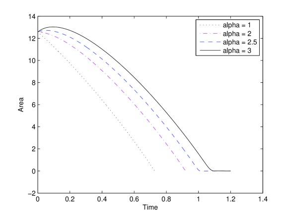
Figure 1: Area of the minimal surface at $r=1$ as a function of flow time, for $\alpha=1$, $2$, $2.5$, and $3$.

In the second run, we probe larger values of $\alpha$, in the hope of seeing expansion of the minimal surface. The results are displayed in figure 2. We use $\alpha$ values all the way up to $\alpha=8$. In each case, collapse eventually commenced, after which there is no evidence for subsequent re-expansion.

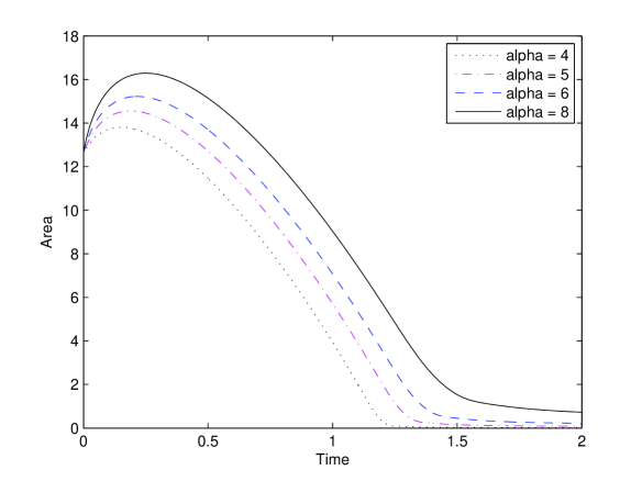
Figure 2: Area of the minimal surface at $r=1$ as a function of flow time, for $\alpha=4$, $5$, $6$, and $8$.

However, at large $\alpha$, the expansion appears eventually to slow and halt. At such values, as the evolution proceeds, sectional curvature becomes highly concentrated at the minimal surface, manifested as a large value of the second spatial derivative of the area $S$. This may indicate that a singularity forms before collapse of the minimal surface occurs, but our numerics are not sufficiently reliable when derivatives become large.

Our third graph deals with the case of $n=2$ dimensions. For initial data derived from the form of (4.1) with $\alpha>0$, the initial scalar curvature will always be negative in 2 dimensions (as is the case in any dimension when $\alpha>n-2$, so each curve in figure 3 will initially expand. By (2.20), we do not have a collapsing upper barrier function for any $\alpha$, but it is still possible in principle that collapse could occur. We find no collapse, despite running for much longer times than for the higher-dimensional cases.

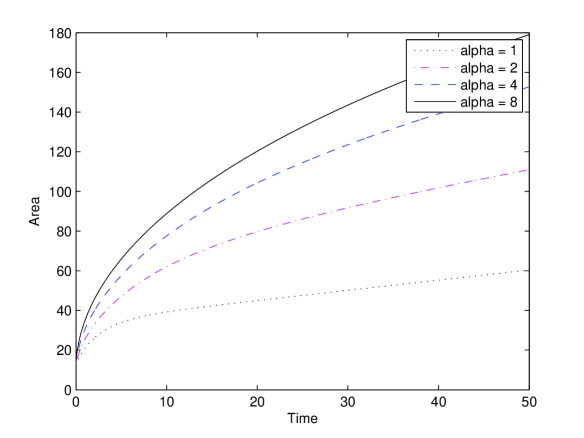
Figure 3: Area of the minimal surface in $n=2$ dimensions as a function of flow time. The initial data are again given by (4.6, 4.7) with $n=2$ and various values of $\alpha$.

The numerical integrations were performed with MATLAB’s “pdepe” integration routine for partial differential equations. We performed several tests of the validity of the code. From equations (3.10), (4.6), and (4.7), we compute $\frac{\partial S}{\partial t}(0,1)=4\pi(\alpha-2)$. This serves to define our unit of time, but also serves as a test of validity of the code, in the sense that the initial derivative should be linear in alpha and zero at $\alpha=2$. This is verified by figure 4, which presents a close-up of the evolution near the initial time.

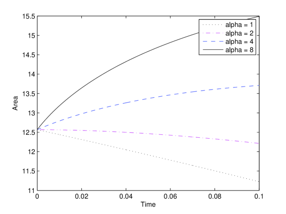
Figure 4: Area of the minimal surface at $r=1$ as a function of flow time for times close to zero, for $\alpha=1$, $2$, $4$, and $8$.

For example, at $\alpha=2$ the slope is zero initially.

As additional verification, we vary the dimension, using initial data for which the scalar curvature obeys $R(0,r)=0$ in each case. The initial data may therefore be regarded as the metric on a moment of time symmetry in an $(n+1)$-dimensional Schwarzschild-Tangherlini exterior spacetime. We therefore use the evolution equations (3.6–3.8) with arbitrary $n\geq 3$ and set $\alpha=n-2$ in (4.6, 4.7). For these runs, we normalize the initial area of the minimal surface to be $2\pi^{n/2}/\Gamma(n/2)$. It is easy to verify, using equation (2.8), and the fact that $R(0,r)=0$ for such data (and thus $R(t,r)\geq 0$ by the maximum principle), that for asymptotically flat boundary conditions the area of the minimal surface will be bounded above at all times by

$$S(t,0)\equiv|\Sigma|\leq\frac{2\pi^{n/2}}{\Gamma(n/2)}\exp\left[-\frac{1}{2}(n-1)(n-2)t\right],\ n\geq 3.$$ (4.11)

This should therefore give an indication of the effect of our boundary condition at finite $r=r_{c}$, which we typically pick to be at $r_{c}=10$ (where $r=1$ is the minimal sphere). The results are depicted in figure 5.

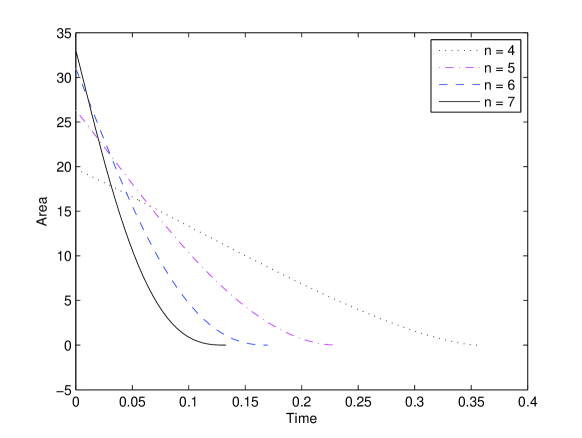
Figure 5: Area of the minimal surface at $r=1$ as a function of flow time for initial data give by a time-symmetric slice of an $(n+1)$-dimensional exterior Tangherlini metric for $n=4$, $5$, $6$, and $7$.

A further technical check concerns the choice of different Hamilton-DeTurck flow. For this, we return to (3.4) and this time choose the flat background, so $\psi=0$ in the evolution equations. The result is displayed in figure 6.

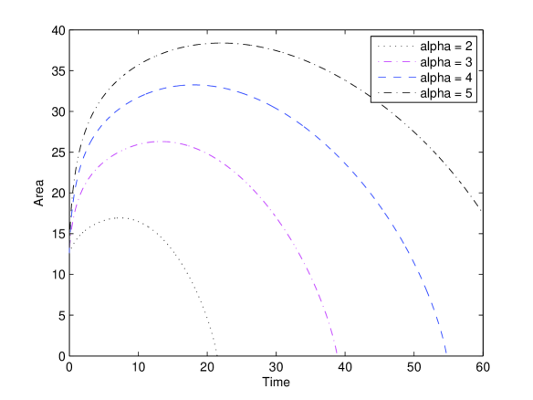
Figure 6: Area of the minimal surface at $r=1$ as a function of flow time, for $\alpha=2$, $3$, $4$, and $3$. The DeTurck diffeomorphism is generated by the difference between the flowing connection and a flat connection.

The evolutions take much longer to collapse, but collapse occurs just as before, and in fact the code seems more reliable close to the collapse time. We present graphs for small $\alpha$, but we carried out the calculation for larger $\alpha$ as well, with similar results.

5 Discussion

The difference between our results and those of Husain-Seahra may have at least two origins. One is the diffuculty in dealing numerically with the nonparabolic system (3.16, 3.17). Another is the difficulty in numerically modelling fall-off conditions on a noncompact manifold using boundary conditions at a fixed boundary. Parabolic equations exhibit instantaneous action-at-a-distance, though it is typically exponentially suppressed. Our numerical runs appear to produce some positive scalar curvature at the large $r$ boundary, which must be chosen sufficiently distant to suppress the effect on the minimal surface. The effect is shown in figure 7. For the figure, we integrated over $r\in[1,100]$ but chose to display only the portion $r=[90,100]$. At early times we see a small pulse of positive scalar curvature concentrated at infinity, presumably attributable in some way to the boundary condition. As time progresses, the pulse dissipates. The figure shows three times, one shortly after the flow begins, one at around the midpoint in time of the flow, and one just before collapse of the minimal surface. We chose to display $\alpha=3$ but the behaviour is similar for all $\alpha$.

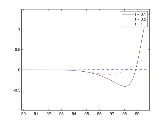
Figure 7: Scalar curvature near the outer boundary at $r=100$ for $\alpha=3$, plotted at three different times, corresponding roughly to $10\%$, $50\%$, and $90\%$ of the time to collapse of the minimal surface. At early times, a disturbance is present near the boundary at $r=100$, but it appears to dissipate without propagating inward. (For comparison, at $r=1$, the initial scalar curvature is $R(0,1)=-4$).

On the other hand, as discussed in subsection 3.2.2, the boundary conditions in [10] imply a concave boundary at $r=r_{c}$ and, concomitantly, appear to produce a source of negative curvature there. Then the maximum principle argument of section 2 would not apply. The critical behaviour observed in [10] may be a property of boundary conditions, rather than evidence for unstable regions in the space of initial data for asymptotically flat metrics.

6 Acknowledgements

We are grateful to Paul Mikula, whose numerical code for a related problem formed the basis from which our code was developed. We thank Viqar Husain and Sanjeev Seahra for discussions. TB was supported by an Undergraduate Summer Research Award from the Natural Sciences and Engineering Research Council of Canada (NSERC). This research was supported by an NSERC Discovery Grant to EW.

References

- [1] M Choptuik, Universality and scaling in gravitational collapse of a massless scalar field, Phys Rev Lett 70 (1993) 9–12.
- [2] B Chow and D Knopf, The Ricci Flow: An Introduction (AMS, Providence, 2004).
- [3] JC Cortissoz, On the Ricci flow in rotationally symmetric manifolds with boundary, PhD thesis (Cornell, 2004, unpublished).
- [4] X Dai and L Ma, Mass under the Ricci flow, Commun Math Phys 274 (2007) 65–80.
- [5] D Garfinkle and J Isenberg, Critical behavior in Ricci flow, in Geometric Evolution Equations, Contemp Math 367 (2005) 103–114, eds S-C Chang, B Chow, S-C Chu, C-S Lin (AMS, Providence) [arxiv.org:math/0306129].
- [6] D Garfinkle and J Isenberg, The modelling of degenerate neck pinch singularities in Ricci flow by Bryant solitons, JMP 49 (2008) 073505 [arxiv:0709.0514].
- [7] L Gulcev, TA Oliynyk, and E Woolgar, On long-time existence for the flow of static metrics with rotational symmetry, preprint [arxiv.org:0911.2037].
- [8] M Gutperle, M Headrick, S Minwalla, and V Schomerus, Space-time energy decreases under world sheet RG flow, JHEP 0301 (2003) 073 [arxiv:hep-th/0211063].
- [9] SW Hawking and GFR Ellis, The large scale structure of space-time (Cambridge, 1973).
- [10] V Husain and SS Seahra, Ricci flows, wormholes and critical phenomena, Class Quantum Gravit 25 (2008) 222002 [arxiv:0808.0880].
- [11] J Jost, Partial Differential Equations, Graduate Texts in Mathematics 214 (Springer, New York, 2002).
- [12] J Morgan and G Tian, Ricci flow and the Poincaré conjecture, Clay Mathematics Monographs Vol 3 (AMS, Providence, 2007).
- [13] TA Oliynyk and E Woolgar, Rotationally symmetric Ricci flow on asymptotically flat manifolds, Commun Anal Geom 15 (2007) 535–568 [arxiv:math/0607438].
- [14] M Simon, A class of Riemannian manifolds that pinch when evolved by Ricci flow, Manuscripta Math 101 (2000) 89–114.
- [15] TJ Willmore, Total curvature in Riemannian geometry (Ellis Horwood, Chicester, 1982); Note on embedded surfaces, Ann St Univ Iasi, Section Ia Matematica 11B (1965) 493–496.