Universality for the focusing nonlinear Schrödinger equation at the gradient catastrophe point:
Rational breathers and poles of the tritronquée solution to Painlevé  I

M. Bertola^†‡, A. Tovbis^♯

^† Centre de recherches mathématiques, Université de Montréal
C. P. 6128, succ. centre ville, Montréal, Québec, Canada H3C 3J7
^‡ Department of Mathematics and Statistics, Concordia University
1455 de Maisonneuve W., Montréal, Québec, Canada H3G 1M8
^♯ University of Central Florida Department of Mathematics
4000 Central Florida Blvd. P.O. Box 161364 Orlando, FL 32816-1364

Abstract

The semiclassical (zero-dispersion) limit of solutions $q=q(x,t,\varepsilon)$ to the one-dimensional focusing Nonlinear Schrödinger equation (NLS) is studied in a scaling neighborhood $D$ of a point of gradient catastrophe ($x_{0},t_{0}$). We consider a certain class of solutions that decay as $|x|\rightarrow\infty$ specified in the text. The neighborhood $D$ contains the region of modulated plane wave (with rapid phase oscillations), as well as the region of fast amplitude oscillations (spikes). In this paper we establish the following universal behaviors of the NLS solutions $q$ near the point of gradient catastrophe: i) each spike has height $3|q{{}_{0}}(x_{0},t_{0})|$ and uniform shape of the rational breather solution to the NLS, scaled to the size $O(\varepsilon)$; ii) the location of the spikes is determined by the poles of the tritronquée solution of the Painlevé  I (P1) equation through an explicit map between $D$ and a region of the Painlevé  independent variable; iii) if $(x,t)\in D$ but lies away from the spikes, the asymptotics of the NLS solution $q(x,t,\varepsilon)$ is given by the plane wave approximation $q_{0}(x,t,\varepsilon)$, with the correction term being expressed in terms of the tritronquée solution of P1. The relation with the conjecture of Dubrovin, Grava and Klein [15] about the behavior of solutions to the focusing NLS near a point of gradient catastrophe is discussed. We conjecture that the P1 hierarchy occurs at higher degenerate catastrophe points and that the amplitudes of the spikes are odd multiples of the amplitude at the corresponding catastrophe point. Our technique is based on the nonlinear steepest descent method for matrix Riemann-Hilbert problems and discrete Schlesinger isomonodromic transformations.

1 Introduction and main results

In this paper we consider the focusing Nonlinear Schrödinger (NLS) equation

$$i\varepsilon\partial_{t}q+\varepsilon^{2}\partial_{x}^{2}q+2|q|^{2}q=0,$$ (1-1)

where $x\in{\mathbb{R}}$ and $t\geq 0$ are space-time variable and $\varepsilon>0$. It is a basic model for self-focusing and self-modulation, for example, it governs nonlinear transmission in optical fibers; it can also be derived as a modulation equation for general nonlinear systems. It was first integrated (with $\varepsilon=1$) by Zakharov and Shabat [39] who produced a Lax pair for it and used the inverse scattering procedure to describe general decaying solutions ($\lim_{|x|\to\infty}q(x,0)=0$) in terms of radiation and solitons. Throughout this work, we will use the abbreviation NLS to mean “focusing Nonlinear Schrödinger equation”.

Our interest in the semiclassical (zero-dispersion) limit ($\varepsilon\to 0$) of NLS stems largely from its modulationally unstable behavior. As shown by Forest and Lee [19], the modulation system for NLS can be expressed as a set of nonlinear PDE with complex characteristics; thus, the system is ill posed as an initial value problem with the initial data (potential) in the form of a modulated plane wave. As a result, this plane wave is expected to break immediately into some other, presumably disordered, wave form when the amplitude and the phase of the potential possess no special properties.

In the case of an analytic initial data, the NLS evolution displays some ordered structure instead of the disorder suggested by the modulational instability (see [30], [37] and [9]), as can be seen on the well-known Figure 1 (from [9]). This figure depicts numerical simulations (obtained by D. Cai) for the absolute value of the solution $q(x,t,\varepsilon)$ of the focusing NLS (1-1) with the initial data of a modulated plane wave $q(x,0,\varepsilon)=A(x)e^{\frac{i}{\varepsilon}\Phi(x)}$, where $A(x)=e^{-{x^{2}}}$ and $\Phi^{\prime}(x)=-\tanh x$,   $\Phi(0)=0$.

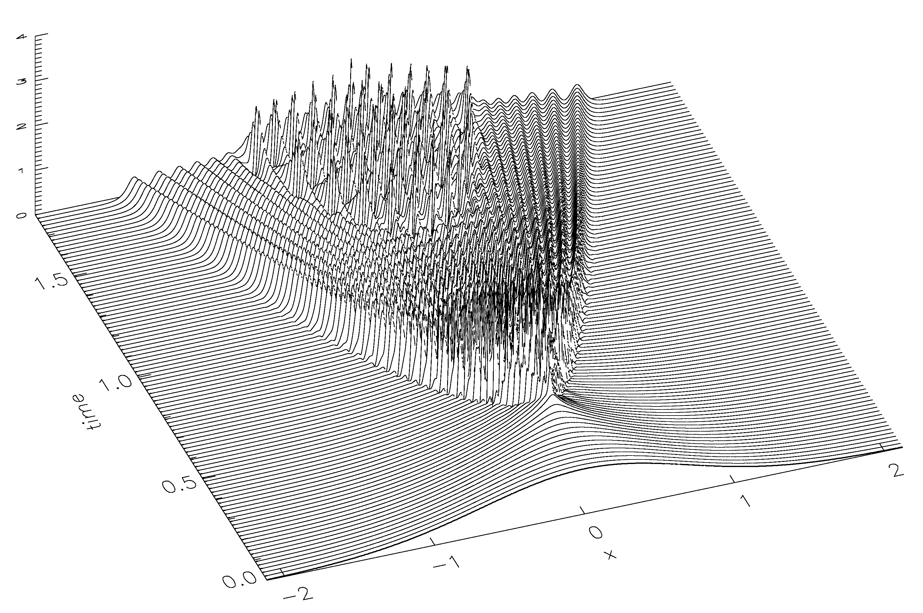
Figure 1: Absolute value $|q(x,t,\varepsilon)|$ of a solution $q(x,t,\varepsilon)$ to the focusing NLS (1-1) versus the space $x$ and the time $t$ coordinates from [9]. Here the potential $q(x,0,\varepsilon)=A(x)e^{\frac{i}{\varepsilon}\Phi(x)}$ with $A(x)=e^{-{x^{2}}}$, $\Phi^{\prime}(x)=-\tanh x$, and $\varepsilon=0.02$.

Figure 1, as well as our numerical simulations shown on Figures 2, 3, clearly identify several spatio-temporal regions of distinct asymptotic regimes of the $q(x,t,\varepsilon)$ in the semiclassical limit $\varepsilon\rightarrow 0$. These regions (called asymptotic regions) are separated by some curves in the $x,t$ plane that are asymptotically independent of $\varepsilon$. They are called breaking curves or nonlinear caustics. In the very first asymptotic region (containing the axis $t=0$) the solution $q(x,t,\varepsilon)$ can be approximated by a slowly modulated plane wave $q_{0}(x,t,\varepsilon)=A(x,t)e^{\frac{i}{\varepsilon}\Phi(x,t)}$. Note that this approximation fails near (the first) breaking curve. A more complicated Ansatz that can be expressed in terms of Riemann Theta-functions is required to approximate modulated nonlinear $2n$-phase waves in the asymptotic regions beyond the first breaking curve, where $n$ can be $1,2,3,\cdots$.

A significant progress in the semiclassical asymptotics of the NLS (1-1) was achieved in [25] (pure soliton case) and [35] (pure radiation and radiation with solitons), where the order $O(\varepsilon)$ approximation $q_{0}(x,t,\varepsilon)$ of $q(x,t,\varepsilon)$ was obtained in the first two asymptotic regions. The $O(\varepsilon)$ error estimate is valid uniformly on compact subsets within the corresponding region. In both papers, the inverse scattering problem for the NLS (1-1) was cast as a two by two matrix Riemann-Hilbert Problem (RHP), whose semiclassical asymptotics was obtained through the combination of the nonlinear steepest descent method of P. Deift and X. Zhou ([13]) and the $g$-function mechanism ([12]). The approximation $q_{0}$, obtained in [25], [35], can be described in terms of some hyperelliptic Riemann surface $\mathcal{R}=\mathcal{R}(x,t)$, which depends on $x,t$ but does not depend on $\varepsilon$. The Schwarz symmetry of the focusing NLS implies that the branchpoints and the branchcuts of $\mathcal{R}$ are Schwarz symmetrical. In this context, regions of different asymptotic behavior of $q(x,t,\varepsilon)$ corresponds to the different genera of $\mathcal{R}(x,t)$, and the approximation $q_{0}(x,t,\varepsilon)$ is expressed in terms of the Riemann Theta-functions of $\mathcal{R}$. In the very first (genus zero) region (that contains the line $t=0$), the approximation $q_{0}(x,t,\varepsilon)$ of $q(x,t,\varepsilon)$ is expressed through the branch-point $\alpha(x,t)$ of $\mathcal{R}(x,t)$ as (see [35])

$$q_{0}(x,t,\varepsilon)=A(x,t)e^{\frac{i}{\varepsilon}\Phi(x,t)}=\Im\alpha(x,t)e^{-\frac{i}{\varepsilon}\int^{(x,t)}_{(0,0)}\{2\Re\alpha(\xi,t)d\xi+[4(\Re\alpha(x,\tau))^{2}-2(\Im\alpha(x,\tau))^{2}]d\tau\}}+O(\varepsilon),$$ (1-2)

We will often refer to this $q_{0}$ as a modulated plane wave (or as genus zero) approximation of the solution $q$. The next asymptotic region (behind the first breaking curve), studied in [25] and [35], corresponds to $\mathcal{R}(x,t)$ of genus two; the corresponding approximation $q_{0}$ in this region has the form of a modulated nonlinear $2$-phase wave.

The approximation formulae in the higher genera regions (genus $4,6,$ etc.) are, in a certain sense, similar to that in the genus two region (the existence of such regions, though, remains a challenging question, see [28] for recent progress in this direction). However, approximation near breaking curves, to our best knowledge, remained to be studied. The first breaking curve consists generically of two smooth branches that form a wedge (tip) when joining together, see Figures 2, 3. In the recent paper [5], we constructed the approximation near the smooth parts (branches) of the first breaking curve: it consists of the modulated plane wave approximation $q_{0}$ from the genus zero region plus correction terms. The shape of the corrections is depicted on Figure 4. They form ranges of peaks and depressions aligned along the breaking curves, see Subsection 1.1. However, the origin of these ranges of peaks and depressions (spikes and anti-spikes) that is, description of the approximation at the tip of the breaking curve, remains somewhat of a mystery. The main goal of the present paper is to describe the mechanism of formation of the spikes, to derive the formula for approximation around the tip of the breaking curve and to prove the corresponding error estimates.

The summary of our findings can be stated as: i) the approximation near the tip consists of the modulated plane wave approximation $q_{0}$ from the genus zero region with $O(\varepsilon^{\frac{2}{5}})$ error term that is expressed in terms of the tritronquée solution to the first Painlevé  equation (P1); ii) evaluated near a pole of the tritronquée solution, the error term becomes commensurable with the leading order term and contribute an order $O(1)$ correction to $q_{0}$; iii) these corrections have the universal shape of a rational (Peregrine) breather, see Figure 12 and their location is determined by the location of poles of the tritronquée solution, see Figure 10.

These facts emphasize the universal role of the tritronquée solution to P1 in the modeling of the transition from a steepening modulated plane wave (gradient catastrophe) to a nonlinear 2-phase wave behavior near the tip of the breaking curve (this transition resembles formation of rogue waves). In fact, the special role of P1 solutions in transitional regimes near critical points was first observed in the context of the orthogonal polynomials with varying exponential weights, see [17] and [18] with some prior physical literature references there, see also [16], where the nonlinear steepest descent method was used for error estimates. In the context of the focusing NLS, the form of the error term containing the tritronquée solution to P1, as well as the localization of all the poles of the tritronquée solution in a certain sector of the complex plane, were conjectured in [15]. In all these results and conjectures, the error terms expressed through solutions of P1 were considered only away from the poles of these solutions. The main contribution of this paper is that we: analyze the error terms both near the poles and away from poles; linked the spikes of an NLS solution with the poles of the tritronquée solution to P1, and; calculated the universal shape of the spikes. The exact localization of the spikes, linked with the localization of the finite poles of the tritronquée, is yet to be established. There are some recent analytical ([24]) and numerical ([31]) results on this issue indicating the triangular shape of the lattice of the poles.

What is the class of solutions to the NLS (1-1) for which our results are valid? As it was mentioned above, our results are based on Deift-Zhou nonlinear steepest descent analysis ([13]) of the semiclassical ($\varepsilon\rightarrow 0$) limit of a matrix RHP that represents the inverse scattering problem for the NLS (1-1). Therefore, in a broad sense, the results of this paper should be applicable to any “generic” solution $q(x,t,\varepsilon)$ for the NLS (1-1) that: a) undergoes a transition from a modulated plane wave to a nonlinear 2-phase wave behavior at a gradient catastrophe point $(x_{0},t_{0})$, and; b) the nonlinear steepest descent method is applicable to the RHP, representing the inverse scattering problem for $q(x,t,\varepsilon)$, in a vicinity of the point $(x_{0},t_{0})$ in the $x,t$ plane. This description, however, cannot be considered satisfactory because of its vagueness. Although, in principle, it is possible to clarify the technical issues involved in the above description, the authors have not found a sufficiently brief and rigorous way of doing so. Therefore, we decided to formulate our results for a much narrower class of solutions $\mathcal{U}$ to the NLS (1-1), defined in Section 2, with some follow up comments regarding the general situation (see Remark 2.1). It was shown in [36] that each $q\in\mathcal{U}$ possesses the following properties: there exists a point of gradient catastrophe $(x_{0},t_{0})$ as required by the condition a) above, and; the nonlinear steepest descent method is applicable not only in a vicinity of $(x_{0},t_{0})$ but also for all $(x,t)$ with $x\in{\mathbb{R}}$ and $t\in[0,t_{0}]$.

A solution $q=q(x,t,\varepsilon)$ of an integrable equations, such as the NLS (1-1), can be defined by its initial (Cauchy) data as well as by its scattering data. Since the input data into the inverse scattering problem (including its RHP formulation) contains the scattering data, it is much more convenient for us to define solutions $q(x,t,\varepsilon)$ through their scattering data. So, to simplify our analysis, the class of solutions $\mathcal{U}$ that we consider consists of solitonless solutions $q(x,t,\varepsilon)$, whose initial datum are defined through their reflection coefficients $r_{0}=r_{0}(z,\varepsilon)$. The choice of $r_{0}$ is such that for every fixed $\varepsilon>0$, $r_{0}$ is continuous on $z\in{\mathbb{R}}$ and has an exponential decay as $z\rightarrow\pm\infty$ (see details in Section 2). Then the corresponding initial data $q=q(x,0,\varepsilon)$ belongs to the weighted $L^{2}({\mathbb{R}})$ with the weight $1+x^{2}$, so the (direct) scattering transform $\mathcal{S}_{\varepsilon}$ between $q$ and $r_{0}$ is well defined, see [40], [41].

Getting into a little bit more details, we can say that, roughly speaking, we consider initial datum $q$ of the form

$$q(x,0,\varepsilon)=\mathcal{S}_{\varepsilon}^{-1}r_{0}(z,\varepsilon)~{}~{}~{}~{}~{}~{}{\rm with}~{}~{}~{}r_{0}(z,\varepsilon)=e^{\frac{2i}{\varepsilon}f_{0}(z)},$$ (1-3)

where functions $f_{0}$, defined by (2-14), (2-15), are called admissible functions. (See Definition 2.2 for the corresponding admissible reflection coefficients $r_{0}$.) Notice that, according to (2-14), (2-15), we consider a special but nevertheless wide class of admissible reflection coefficients. Given an admissible reflection coefficient $r_{0}=r_{0}(z,\varepsilon)$, what do we know about the semiclassical limit of the corresponding initial data $q$? According to [36], for any admissible $r_{0}$ there exist a pair of smooth functions $A(x),\Phi(x)$ with $\lim_{|x|\rightarrow\infty}A(x)=0$ and $\Phi^{\prime}(x)$ having finite limits at $\pm\infty$, such that

$$q(x,0,\varepsilon)=A(x)e^{\frac{i}{\varepsilon}\Phi(x)}+O(\varepsilon)~{}~{}~{}~{}~{}{\rm as}~{}~{}\varepsilon\rightarrow 0$$ (1-4)

uniformly on compact subsets of ${\mathbb{R}}$. It would be certainly nice to remove the “compact subsets” condition from (1-4), but this is the subject of a different project. It could be added here that in numerical/experimental applications (like [33]), the data is always truncated to a finite interval and hence the control of the approximation over compact sets in these cases is sufficient.

Example 1.1

To illustrate the above discussion, consider the solitonless initial data

$$\hat{q}(x,0;\varepsilon):={\frac{1}{\cosh(x)}}e^{-\frac{\mu i}{\varepsilon}{\ln\cosh x}+i\pi},$$ (1-5)

$\mu\geq 2$, whose reflection coefficient $\hat{r}_{0}(z,\varepsilon)$ is explicitly known ([35]). For example,

$$\hat{r}_{0}(z)=-i\varepsilon 2^{-\frac{2i}{\varepsilon}}\frac{\Gamma(\frac{1}{2}+\frac{i}{\varepsilon}(z-1))\Gamma^{2}(\frac{1}{2}-\frac{iz}{\varepsilon})}{\Gamma^{2}(-\frac{i}{\varepsilon})\Gamma(\frac{1}{2}+\frac{i}{\varepsilon}(z-1))},~{}~{}~{}\Im z\geq 0,$$ (1-6)

when $\mu=2$. Notice that $\hat{r}_{0}(z)$ is not an admissible reflection coefficient since, for example, $\hat{f}_{0}(z,\varepsilon)=-\frac{i\varepsilon}{2}\ln\hat{r}_{0}(z,\varepsilon)$ has logarithmic singularities at the poles $z_{n}=1+(n+\frac{1}{2})ni$, $n\in{\mathbb{N}}$, of $\hat{r}_{0}(z)$. On the other hand, retaining the first two terms in the small $\varepsilon$ expansion of $\hat{f}_{0}(z,\varepsilon)$ (calculated by the Stirling formula), we obtain

$$f_{0}(z):=\lim_{\varepsilon\rightarrow 0}\hat{f}_{0}(z,\varepsilon)+\frac{\pi\varepsilon}{2}=(1-z)\left[i\frac{\pi}{2}+\ln(1-z)\right]+z\ln z+\ln 2+\frac{\pi\varepsilon}{2},$$ (1-7)

where $\Im z\geq 0$ and $z\neq 1$. With a proper choice of logarithmic branches ([35]), one can check that $w(z)=\Im f_{0}(z){\rm sign}(1-z)=\frac{\pi}{2}|1-z|$, $z\in{\mathbb{R}}$, is an admissible function (Definition 2.1). Then a corresponding reflection coefficient $r_{0}$, defined on $z\in[-1,1]$ as $r_{0}(z,\varepsilon)=e^{\frac{2i}{\varepsilon}f_{0}(z)}$ (see Definition 2.2 for full details), is an admissible reflection coefficient. It was proven in [35] that $q(x,0,\varepsilon)=\mathcal{S}^{-1}_{\varepsilon}r_{0}(z,\varepsilon)$ is an order $O(\varepsilon)$ approximation of $\hat{q}(x,0,\varepsilon)$ as $\varepsilon\rightarrow 0$ on compact subsets of ${\mathbb{R}}$.

Generalizing on the above example, one can consider the class of solutions $q\in\mathcal{U}$ as obtained by replacing actual reflection coefficients $\hat{r}_{0}=\mathcal{S}_{\varepsilon}\hat{q}$ of solitonless initial datum of the form $\hat{q}(x,0,\varepsilon)=A(x)e^{\frac{i}{\varepsilon}\Phi(x)}$ by their small $\varepsilon$ admissible approximations $r_{0}=r_{0}(z,\varepsilon)$. Although there is no proof that the solution $q(x,t,\varepsilon)$ defined by the initial data $q(x,0,\varepsilon)=\mathcal{S}^{-1}_{\varepsilon}r_{0}(z,\varepsilon)$ will stay close to $\hat{q}(x,t,\varepsilon)$ on some time interval $t\in[0,t_{*}]$, $t_{*}>0$, the idea of replacing an actual scattering data with its convenient small $\varepsilon$ approximation was widely used in semiclassical asymptotics of integrable systems starting with the pioneering papers [27] for the Korteweg - de Vries equation and through all analytical studies for the NLS, sine-Gordon, modified NLS that the authors aware of ([25],[35],[3], [14]). The only notable exception is [20], where a very simple form of the initial data allows for direct estimates.

Figure 2: Absolute value $|q(x,t,\varepsilon)|$ of a solution $q(x,t,\varepsilon)$ to the focusing NLS (1-1) versus $x,t$ coordinates. Here $q(x,0,\varepsilon)=A(x)e^{\frac{i}{\varepsilon}\Phi(x)}$ with $A(x)=e^{-{x^{2}}}$, $\Phi^{\prime}(x)=\tanh x$ and $\varepsilon=0.03$.

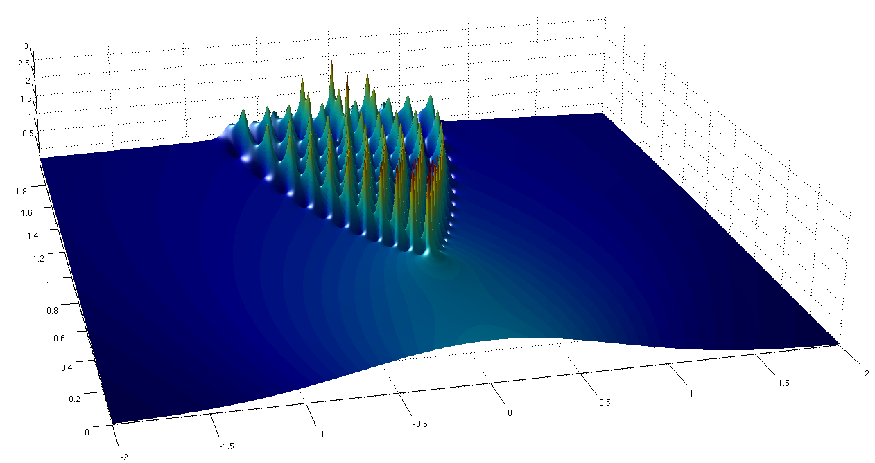
Figure 3: Absolute value $|q(x,t,\varepsilon)|$ of a solution $q(x,t,\varepsilon)$ to the focusing NLS (1-1) versus $x,t$ coordinates. Here $q(x,0,\varepsilon)=A(x)e^{\frac{i}{\varepsilon}\Phi(x)}$ with $A(x)=e^{-{x^{2}}}$, $\Phi^{\prime}(x)=\tanh x$ and $\varepsilon=0.03$.

1.1 Semiclassical limit along the breaking curve

A detailed study of asymptotic behavior of $q(x,t,\varepsilon)$ along the first breaking curve (a neighborhood of the tip of this curve was excepted) together with error estimates were conducted in our previous work [5]. Considering one of the pieces of the breaking curve (to the left, $x<0$, or to the right, $x>0$, from the tip $x_{0}=0,t_{0}\approx\frac{1}{2}$, see Fig. 3, where the $x,t$-plane is shown upside-down), we introduced two scaled coordinates $\vartheta$ measuring lengths of order $\mathcal{O}(\varepsilon)$ in the tangent direction to the breaking curve, and $\kappa$ measuring lengths of order $\mathcal{O}(\varepsilon\ln\varepsilon)$ in the transversal direction. In these coordinates $\kappa>0$ was the interior of the oscillatory region (see Fig. 2, 4). The shape of the oscillations in the $\kappa,\vartheta$-plane is depicted on Fig. 4.

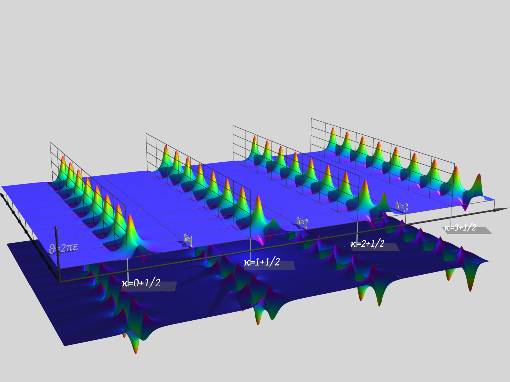
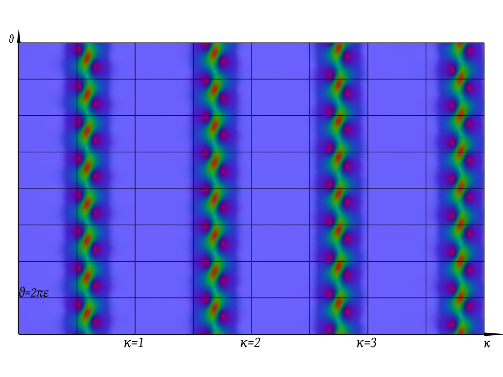
Figure 4: The graphs depict a typical ratio $\frac{\tilde{q}(x,t,\varepsilon)}{q_{0}(x,t,\varepsilon)}$ in a vicinity of a regular point on the breaking curve, where $q_{0}$ is the genus zero approximate solution and $\tilde{q}$ is the leading order approximation near the breaking curve, constructed in [5]. The graph is shown in the variables $\theta,\varkappa$ and the scale is not uniform: $\varkappa$ measures distances in the scale $\varepsilon|\ln\varepsilon|$ whereas $\theta$ in the scale $\varepsilon$. The distance between consecutive “ranges”, should be much longer than the separation of the neighboring peaks within the same range. The typical size of the hills is $\varepsilon$ in all directions while the separation in the longitudinal direction is $\varepsilon|\ln\varepsilon|$. This picture is consistent with a full–blown genus-two regime, where the solution is quasi-periodic at the scale $\varepsilon$: as we progress into the genus-2 region the separation reduces to the natural scale $\varepsilon$. If we were to plot this in the $(x,t)$ plane the only difference would be a linear change of coordinates and the “ranges” would be parallel to the breaking curve.

The tip-point $x_{0},t_{0}$ of the breaking curve is called a point of gradient catastrophe, or elliptic umbilical singularity ([15]).) It is evident from the numerical simulations shown on Fig. 2 and Fig. 3, as well as from the analysis of the spectral plane (presented below), that the behavior of the solution $q(x,t,\varepsilon)$ at the tip of the breaking curve is very different from the behavior elsewhere on the breaking curve.

The main goal of this paper is to analyze the leading order asymptotic behavior of the solution $q(x,t,\varepsilon)$ on and around this special point of transition. More precisely we will examine a neighborhood $D$ of $(x_{0},t_{0})$ that is shrinking at the rate $\mathcal{O}(\varepsilon^{\frac{4}{5}})$ as $\varepsilon\rightarrow 0$. As the first step, we construct a map $v=v(x,t,\varepsilon)$, that maps $D$ onto a bounded disk $V\in{\mathbb{C}}$, where $V$ is independent of $\varepsilon$ and $v(x_{0},t_{0},\varepsilon)=0$. It turns out that the leading order behavior of $q(x,t,\varepsilon)$ in $D$ can be conveniently described through a specific tritronquée solution (see Section 4.2.1) to the Painlevé  I (P1) equation

$$y^{\prime\prime}(v)=6y(v)^{2}-v.$$ (1-8)

That is why the map $v(x,t,\varepsilon)$ and the complex $v$-plane will be referred to as the Painlevé  coordinatization of $D$ and the Painlevé  plane respectively. Note that the map $v(x,t,\varepsilon)$ near the point of gradient catastrophe plays a similar role to the map $S(x,t,\varepsilon)$ for the rest of the breaking curve.

The point of gradient catastrophe $(x_{0},t_{0})$ for a solution $q\in\mathcal{U}$ of the NLS (1-1) can be defined in terms of the space-time (physical) variables $(x,t)$ as the point, where the genus zero approximation (1-2) of the solution $q(x,t,\varepsilon)$ develops an infinite $x$-derivative in $A(x,t)$ and/or in $\Phi_{x}(x,t)$ (while $A(x,t)$ and $\Phi_{x}(x,t)$ stay finite). In terms of the time evolution of the spectral data (see Fig. 6 below), the point of gradient catastrophe is the point where the birth/collapse of the new main arc (band) happens exactly at the end of an existing main arc (see Fig. 6).

As it was mentioned above, the asymptotics of $q(x,t,\varepsilon)$ within the region of a given genus is given explicitly in terms of the Riemann Theta-functions, associated with $\mathcal{R}(x,t)$, with the accuracy $\mathcal{O}(\varepsilon)$, see [35], [25]. (In the case of genus zero, see (1-2).) The leading order approximation $\tilde{q}(x,t,\varepsilon)$ of $q(x,t,\varepsilon)$ in order $O(\varepsilon\ln\varepsilon)$ strips around left and right branches of the breaking curve, found in [5], has the accuracy $O(\sqrt{\varepsilon})$.

1.2 Description of results

We provide the leading order behavior together with the accuracy estimate in the whole domain $D$ around the point of gradient catastrophe $x_{0},t_{0}$, that include the oscillatory part of $D$. The following notations are useful in describing our results.

Let: $V$ denote a compact neighborhood of the origin $v=0$ of the independent variable $v$ of the Painlevé transcendent (for example a bounded disk of arbitrary large but fixed radius); $V_{p}=\{v_{p,1},\cdots,v_{p,N}\}\subset V$ denote the set of poles of the tritronquée solution $y(v)$ in $V$; $B_{\delta,j}$ denote the disk of radius $\delta>0$ centered at $v_{p,j}$, $j=1,\cdots,N$, $B_{\delta}=\cup_{1}^{N}B_{\delta,j}$ and $K_{\delta}=V\setminus B_{\delta}$. Denoting

$$a=-\frac{1}{2}\Phi_{x}(x_{0},t_{0}),~{}~{}~{}~{}~{}~{}b=A(x_{0},t_{0}),$$ (1-9)

(so that, according to (1-2), $a+ib=\alpha(x_{0},t_{0})$), we prove:

1. (Thm. 6.3) There is a one to one correspondence between the poles of the tritronquée solution $y(v)$ within $V$ and the spikes of the NLS solution $q$ within $D$. Each spike is centered at the corresponding $(x_{p,j},t_{p,j})=v^{-1}(v_{p,j})$, where

   $$v(x,t,\varepsilon)=\frac{e^{-i\pi/4}}{\varepsilon^{\frac{4}{5}}}\sqrt{\frac{2b}{C}}\left[x-x_{0}+2(2a+ib)(t-t_{0})\right]\left(1+\mathcal{O}(\varepsilon^{\frac{2}{5}})\right)$$ (1-10)

   uniformly in $D$, with the nonzero constant $C$ explicitly defined by (3-48) in terms of the scattering data;

2. Each spike has the fixed height of $3|q_{0}(x_{0},t_{0},\varepsilon)|+O(\varepsilon^{1/5})$, where $q_{0}$ is the genus zero approximation of $q$, i.e., the height of each spike is three times the amplitude at the gradient catastrophe, see Theorems 6.2, 6.3;

3. Each spike has the universal shape of the (scaled) rational breather solution to the NLS eq. (1-1), see Fig. 12, i.e,

   $$q(x,t,\varepsilon)={\rm e}^{\frac{i}{\varepsilon}\Phi(x_{p},t_{p})}Q_{br}\left(\frac{x-x_{p,j}}{\varepsilon},\frac{t-t_{p,j}}{\varepsilon}\right)(1+\mathcal{O}(\varepsilon^{\frac{1}{5}})),$$ (1-11)

   where the rational breather

   $$Q_{br}(\xi,\eta)={\rm e}^{-2i\left(a\xi+(2a^{2}-b^{2})\eta\right)}b\,\left(1-4\frac{1+4ib^{2}\eta}{1+4b^{2}(\xi+4a\eta)^{2}+16b^{4}\eta^{2}}\right)$$ (1-12)

   satisfies the NLS eq. (1-1) with space-time variables $\xi,\eta$. This breather approximation of the spike is valid in the domain $\tilde{B}_{j}=v^{-1}(B_{\delta,j})$ of $(x_{p,j},t_{p,j})$, where $\delta=O(\varepsilon^{1/5})$, see Theorems 6.2) and [5]. The size of each spike in the physical plane (the size of $\tilde{B}_{j}$) is thus $O(\varepsilon)$, which is consistent with the size of spikes along the breaking curve (away from $(x_{0},t_{0})$) and within the bulk of the genus two region, see above. The two zeroes (“roots”) and the maximum of each breather, shown on Fig. 12, occur at the same time (within the accuracy of our approximation). We note here that this universal shape is a completely new result, which, to our best knowledge, was never even conjectured or observed numerically.

4. In Thm. 5.2 we show that if $\delta>0$ is a small fixed number then

   $$q(x,t,\varepsilon)=\left(b-2\varepsilon^{\frac{2}{5}}\Im\left(\frac{y(v)}{C}\right)+\mathcal{O}(\varepsilon^{\frac{3}{5}})\right)\times$$ (1-13)

   $$\exp\frac{2i}{\varepsilon}\left[\frac{1}{2}\Phi(x_{0},t_{0})-\left(a(x-x_{0})-(2a^{2}-b^{2})(t-t_{0})\right)+\varepsilon^{\frac{6}{5}}\Re\left(\sqrt{\frac{2i}{Cb}}H_{I}(v)\right)\right]$$ (1-14)

   uniformly in $\hat{K}_{\delta}=v^{-1}(K_{\delta})$ (i.e. uniformly over compact sets of the $v$ plane that do not contain any pole), where $C$ is a nonzero constant explicitly given by (3-48), $y(v)=y(v(x,t,\varepsilon))$ is the tritronquée solution and $H_{I}=\frac{1}{2}(y^{\prime}(v))^{2}+vy(v)-2y^{3}(v)$. Equation (1-13) is consistent with the conjecture of [15] (see Remark 5.3), although that conjecture is formulated for a different class of solutions (defined through their initial data).

5. If $\delta=O({\varepsilon^{\nu}})$, where $\nu\in(0,\frac{1}{5})$, and $\hat{K}_{\delta}=v^{-1}(K_{\delta})$, then equation (1-13) will be uniformly valid in $\hat{K}_{\delta}$ provided that $\varepsilon^{\frac{1}{5}}$ in the error term will be replaced by $\varepsilon^{\frac{1}{5}-\nu}$, i.e.

   $$q(x,t,\varepsilon)=\left(b-2{\varepsilon^{\frac{2}{5}}}\Im\left(\frac{y(v)}{C}\right)+\mathcal{O}(\varepsilon^{\frac{3}{5}-3\nu})\right)\times$$ (1-15)

   $$\exp\frac{2i}{\varepsilon}\left[\frac{1}{2}\Phi(x_{0},t_{0})-\left(a(x-x_{0})-(2a^{2}-b^{2})(t-t_{0})\right)+{\varepsilon^{\frac{6}{5}}}\Re\left(\sqrt{\frac{2i}{Cb}}H_{I}(v)\right)\right].$$ (1-16)

   Note that – since $y(v)$ has a double pole and $H_{I}(v)$ a simple pole – the term $y(v)$ is actually of order $\varepsilon^{-2\nu}$ and $H_{I}(v)$ of order $\varepsilon^{-\nu}$; clearly the description in terms of the tritronquée cannot be pushed “too close” to the pole/spike.

Note that the results above hold uniformly within the specified regions $\cup_{j}\tilde{B}_{j}$ and $\tilde{K}_{\delta}$ and hence are not sensitive to the actual location of the poles of the tritronquée solution $y(v)$. That is to say that the actual behavior of a solution $q$ near the point of gradient catastrophe depends on the location of the spikes and hence of the poles of $y(v)$, but does not affect the description of the individual spike.

We also make the Conjecture 6.1 that the amplitudes of the spikes near any (degenerate) gradient catastrophe point in the genus zero phase are odd multiples of the amplitude at the point itself. In addition we can speculate that the shape of the spikes in the higher-degeneracy cases should be related to the higher rational breathers recently investigated in [1].

Among other results obtained in this paper we mention the proof that the two branches of the breaking curve form a corner (wedge) at the point of gradient catastrophe $(x_{0},t_{0})$ and give explicit expression, see (3-61), of the angle between the breaking curve in terms of $C$ and $\alpha(x_{0},t_{0})$. We further prove that the map $v(x,t,\varepsilon)$ maps this corner into the sector $\frac{2\pi}{5}<\arg v<\frac{4\pi}{5}$ of the complex $v$-plane, see Fig. 10. This is consistent with another conjecture, stated in [15]: all the poles of the tritronquée solution $y(v)$ are contained within the sector $\frac{2\pi}{5}<\arg v<\frac{4\pi}{5}$. This is a longstanding question in the theory of Painlevé  equations. According to our results, the set of spikes near the point of gradient catastrophe is, in fact, the visualization of the poles of the tritronquée solution $y(v)$ to P1. In this sense numerical simulations, shown on Fig. 2 and 3 (as well as similar computations in other papers), are consistent with the conjecture from [15], although they do not amount to a proof. The very first real pole of the real-analytic tritronquée solution was numerically calculated in [24]. Applied to our case, the result of [24] implies that the very first pole $v_{p,1}$ of $y(v)$ on the ray $\arg v=\frac{3\pi}{5}$ has $|v_{p,1}|\approx 2.38$. Using (1-10), we calculate $(x_{p,1},t_{p,1})=(0,2.79126)$ for the NLS evolution of the initial data $q(x,0,\varepsilon)={\rm sech}x$. Numerical simulation of this evolution with $\varepsilon=\frac{1}{33}$ shows the first spike at $t_{s}\approx 2.8$, which is in a very good agreement with $t_{p,1}$, see Example 6.2 and Fig. 13

Remark 1.1

Statement 4 from the above list is consistent with Dubrovin’s conjecture [15] for solutions $q\in\mathcal{U}$.

While reducing the (original) matrix RHP, associated with the inverse scattering transform, to the model RHP, the error is controlled through the so-called local parametrices. At the regular points $(x,t)$ in the physical plane, these parametrices can be constructed through the Airy functions. As we show in Section 4, at the point of gradient catastrophe $(x_{0},t_{0})$, the parametrix $\mathcal{P}$ is constructed through the tritronquée solution $y(v)$ of the P1. It is well known that Painlevé equations can be expressed as conditions of isomonodromic deformations for certain rational $2\times 2$ systems of ODEs with rational coefficients [23, 21]. The parametrix $\mathcal{P}$ at the point of gradient catastrophe is built through the fundamental solution $\Psi(\xi;v)$ to the system of ODEs associated with the P1. The occurrence of parametrices built out of Painlevé associated linear systems is not unexpected here, as they often appear in various RHPs related to random matrices/orthogonal polynomials, for example:

• The case of random matrices with a soft-edge where the density vanishes to order $(z-\alpha)^{2k+1/2}$, corresponding to the even P1 hierarchy [11];

• The case of random matrices where a spectral band splits into two (P2 equation [6] and hierarchy);

• The trailing edge of the region of oscillations in the small–dispersion limit of KdV [10] (PII equation).

The novelty of our work lies in the fact that the matrix $\Psi(\xi;v)$, and thus, the parametrix $\mathcal{P}$, is not defined (has poles) at the poles $v_{p}\in V$ of the tritronquée solution $y(v)$. To our best knowledge, this paper contains the first example of parametrices with singularities, that were successfully used to control the errors at and around the singularities.

Solving the RHP at or near the pole $v_{p}$ of $y(v)$, i.e., studying the shape of the spike, require several additional steps, which can be briefly listed as:

• Factorization $\Psi(\xi;v)=G(\xi,v)\hat{\Psi}(\xi,v)$, where $G(\xi,v)$ is a “simple” matrix with singularity at $v=v_{p}$, and $\hat{\Psi}(\xi,v)$ is regular at $v=v_{p}$. This factorization was introduced by D. Masoero in [29]. The existence of the limit of $\hat{\Psi}(\xi,v)$ as $v\rightarrow v_{p}$ that is uniform in a certain region of the spectral $\xi$-plane (see Appendix A), is an important part in establishing the shape of spikes;

• Construction of $\Psi_{1}$, solution of a modified model RHP, that is needed at the poles $v=v_{p}$ of the tritronquée solution $y(v)$. $\Psi_{1}$ was obtained by means of the discrete Schlesinger isomonodromic deformations of $\Psi_{0}$, solution to the “standard” model RHP. This type of deformations were used, for example, in [4, 5];

• Construction of the new parametrix $\mathcal{P}_{1}$ for the modified model RHP, using $\hat{\Psi}(\xi,v)$. The formula $3b+O(\varepsilon^{1/5})$ for the height of spikes follows immediately from $\mathcal{P}_{1}$;

• Additional transformation of $\Psi_{1}$, called partial Schlesinger transformation, is used to obtain the shape of the spikes, see (1-11).

Finally, it is clear that our method can be modified to handle higher order (degenerate) gradient catastrophes, where $k$ main arcs, $k>1$, simultaneously emerge from the endpoints of an existing main arc. The parametrices in these cases can be written in terms of the higher members of the P1 hierarchy, and one should expect the height of the spikes to be $2k+1$ times the amplitude at the point of gradient catastrophe.

To summarize our results about the typical behavior of a solution $q=q(x,t,\varepsilon){\in\mathcal{U}}$ in a full $O(\varepsilon^{\frac{4}{5}})$-scaled neighborhood $D$ around the point of its gradient catastrophe $(x_{0},t_{0})$:

• The poles of the tritronquée solution $y(v)$ that belong to $V$ are mapped into $D$ by the map $(x,t)=v^{-1}(v)$;

• Every pole $v_{p}$ from $V$, wherever in $V$ it is located, generates a spike of the size $O(\varepsilon)$ and of the universal height $3|q_{0}(x_{0},t_{0},\varepsilon)|$ centered around $(x_{p},t_{p})=v^{-1}(v_{p})$. All the spikes have the universal shape of the scaled rational breather;

• In between the spikes, the solution $q$ is approximated by the constant $q(x_{0},t_{0},\varepsilon)$ term with accuracy $O(\varepsilon^{\frac{2}{5}})$, where the correction term is explicitly given in terms of $y(v)$;

• While the actual behavior of $q$ in $D$ depends on where the poles of the tritronquée solution $y(v)$ are located, our universal description of the spikes of $q$ is valid regardless of the location of the poles of $y(v)$.

2 A short review of the zero dispersion limit of the inverse scattering transform

At any time $t$, the inverse scattering problem for a solitonless solution $q=q(x,t,\varepsilon)$ of (1-1) with a fixed (not infinitesimal) $\varepsilon$ is reducible to the following matrix RHP.

Problem 2.1

Find a matrix $\mathbf{\Gamma}(z)$ analytic in ${\mathbb{C}}\setminus{\mathbb{R}}$ such that

$$\mathbf{\Gamma}_{+}(z)=\mathbf{\Gamma}_{-}(z)\left[\begin{array}[]{cc}|r_{0}(z,\varepsilon)|^{2}+1&\overline{r}_{0}(z,\varepsilon){\rm e}^{-\frac{2i}{\varepsilon}\left(2tz^{2}+xz\right)}\\ r_{0}(z,\varepsilon){\rm e}^{\frac{2i}{\varepsilon}\left(2tz^{2}+xz\right)}&1\end{array}\right]\ ,\ \ z\in{\mathbb{R}},$$ (2-3)

$$\mathbf{\Gamma}(z)={\bf 1}+\frac{1}{z}\mathbf{\Gamma}_{1}+\mathcal{O}(z^{-2})\ ,\ \ \ \ z\to\infty,$$ (2-4)

where $r_{0}(z,\varepsilon)$ is the reflection coefficient of $q$. (In the case with solitons, there are additional jumps across small circles surrounding the points of discrete spectrum, see [39].) Then

$$q(x,t,\varepsilon):=-2\left(\mathbf{\Gamma}_{1}\right)_{12}.$$ (2-5)

The jump matrix for the RHP admits the factorization

$$\left[\begin{array}[]{cc}|r|^{2}+1&\overline{r}\\ r&1\end{array}\right]=\left[\begin{array}[]{cc}1&\overline{r}\\ 0&1\end{array}\right]\left[\begin{array}[]{cc}1&0\\ r&1\end{array}\right],$$ (2-12)

where $r=r(z;x,t,\varepsilon)=r_{0}(z,\varepsilon){\rm e}^{\frac{2i}{\varepsilon}\left(2tz^{2}+xz\right)}$.

Inspection of the RHP shows that the matrix $\mathbf{\Gamma}(\overline{z})^{*}$ (where ^∗ stands for the complex–conjugated, transposed matrix) solves the same RHP with the jump matrix $M(z)$ replaced by $M^{-1}(z)$ and hence:

Proposition 2.1

The solution $\mathbf{\Gamma}(z)$ of the RHP for NLS has the symmetry

$$\mathbf{\Gamma}(z)(\mathbf{\Gamma}(\overline{z}))^{*}\equiv{\bf 1}~{}.$$ (2-13)

We shall now specify the set $\mathcal{U}$ of solution to the NLS (1-1); it consists of solitonless solutions with admissible reflection coefficients ([36]), as defined below.

Figure 5: Typical graph of $w(z)$.

Definition 2.1

An absolutely continuous, piecewise $C^{1}$, real function $w(\zeta)$ with a locally square-integrable derivative is admissible if it satisfies the following additional conditions:

1. there exists $\mu_{-}<0<\mu_{+}$ such that $w(\zeta)$ is positive on $(\mu_{-},\mu_{+})$ and negative on the union $(-\infty,\mu_{-})\cup(\mu_{+},\infty)$;

2. $w^{\prime}(\mu_{-}\pm 0)>0$ and $w^{\prime}(\mu_{+}\pm 0)<0$;

3. $\exists k\geq 0$ such that $w^{\prime}(\zeta)=\mp k+o(1)$ as $\zeta\rightarrow\pm\infty$;

4. ${\rm sign}(\mu_{+}-\zeta)w^{\prime}(\zeta)-k\in L^{1}({\mathbb{R}})$.

Given an admissible function $w(\zeta),~{}\zeta\in{\mathbb{R}}$, we construct the function $f_{0}(z)$ (unique up to a real constant), that is analytic and Schwarz reflection invariant in ${\mathbb{C}}\setminus{\mathbb{R}}$ in the following way: first, using the Cauchy transform, we construct $f^{\prime}_{0}(z)$ by

$$f_{0}^{\prime}(z)=ik{\rm sign}(\Im z)+\frac{1}{\pi}\int_{-\infty}^{\infty}\frac{{\rm sign}(\mu_{+}-\zeta)w^{\prime}(\zeta)-k}{\zeta-z}d\zeta;$$ (2-14)

then $f_{0}(z)$ is an antiderivative of $f^{\prime}_{0}(z)$ satisfying

$$\Im f_{0}(\zeta)_{+}=w(\zeta){\rm sign}(\mu_{+}-\zeta),~{}~{}~{}~{}~{}~{}~{}\zeta\in{\mathbb{R}},$$ (2-15)

where the subscripts $\pm$ indicate limiting values on the real axis from the upper/lower complex half plane respectively. Notice also that: $\Re f^{\prime}_{init}(\zeta)_{\pm}=\mathcal{H}[{\rm sign}(\mu_{+}-\zeta)w^{\prime}(\zeta)-k]$ for almost every $\zeta\in[\mu_{-},\mu_{+}]$ (here $\mathcal{H}$ denotes the Hilbert transform); as $z\rightarrow\infty$,

$$f^{\prime}_{0}(z)=ik{\rm sign}(\Im z)-\frac{1}{z\pi}\int_{-\infty}^{\infty}[{\rm sign}(\mu_{+}-s)w^{\prime}(s)-k]ds+o(z^{-1})~{},$$ (2-16)

and; $\Im f_{0}(z)$ has a jump across the real axis given by

$$f_{0}(\zeta)_{+}-f_{0}(\zeta)_{-}=2i{\rm sign}(\mu_{+}-\zeta)w(\zeta),\ \ \ \ \zeta\in{\mathbb{R}}.$$ (2-17)

Definition 2.2

A reflection coefficient $r_{0}$ continuous on ${\mathbb{R}}$ is called admissible if there exists an admissible function $w(\zeta),~{}\zeta\in{\mathbb{R}}$, such that

$$\left\{\begin{array}[]{cc}r_{0}(\zeta,\varepsilon)=e^{-\frac{2i}{\varepsilon}f_{0}(\zeta)_{+}},\ \ \mbox{when $\zeta\in[\mu_{-},\mu_{+}]$},\\ |r_{0}(\zeta,\varepsilon)|\leq ce^{-\frac{1}{\varepsilon}{\min\{c_{1}|\zeta-\mu_{\pm}|,c_{2}\}}},\ \ \mbox{when $\zeta\notin[\mu_{-},\mu_{+}]$},\end{array}\right.$$ (2-18)

where $c,\ c_{1},\ c_{2}$ are some positive constants and $f_{0}$ is as described above.

In other words, a reflection coefficient $r_{0}$ is admissible if: A) it is exponentially decaying (with respect to $\varepsilon$) outside some interval $[\mu_{-},\mu_{+}]$ and exponentially growing inside this interval; B) for any fixed $\varepsilon>0$ it is exponentially decaying as $\zeta\rightarrow\pm\infty$; C) the values of $f_{0}(\zeta)=\frac{1}{2}i\varepsilon\ln r_{0}(\zeta)$ on $[\mu_{-},\mu_{+}]$ are boundary values of some analytic in the upper half-plane function $f_{0}(z)$, such that (2-15) and (2-16) hold, where $w(\zeta)$ and $k$ satisfy all the requirements in Definition 2.1.

Definition 2.3

Let $\mathcal{S}_{\varepsilon}$ denote the (direct) scattering transform for solitonless initial data of the NLS (1-1). The set $\mathcal{U}$ of solutions $q(x,t,\varepsilon)$ to (1-1) is the set of solitonless solutions with initial data of the form $q(x,0,\varepsilon)=S^{-1}_{\varepsilon}r_{0}(z,\varepsilon)$, where $r_{0}(z,\varepsilon)$ are admissible reflection coefficients.

The most advanced results to our knowledge about the correspondence between the initial and the scattering data for the focusing NLS (with a fixed $\varepsilon$) can be found in [40], [41]. According to them, since an admissible reflection coefficient $r_{0}$ (with a fixed $\varepsilon>0$) is continuous, piece-wise differentiable on ${\mathbb{R}}$ and is exponentially decaying at $\zeta\rightarrow\pm\infty$, the corresponding initial data $q(x,0,\varepsilon)$ belongs to the weighted $L^{2}({\mathbb{R}})$ with the weight $1+x^{2}$. Moreover, the additional assumption $r_{0}\in C^{\infty}({\mathbb{R}})$ would imply that $q(x,0,\varepsilon)$ is in the Schwarz class. In the semiclassical limit, one can take advantage of the steepest descent method for RHP (2.1)-(2-4) to prove (see [36]) that a solution $q\in\mathcal{U}$ has the modulated plane wave (genus zero) approximation $q(x,t,\varepsilon)=q_{0}(x,t,\varepsilon)+O(\varepsilon)$ that is valid uniformly on the compact subsets of the genus zero region. Here $q_{0}(x,t,\varepsilon)=A(x,t)\exp\{\frac{i}{\varepsilon}\Phi(x,t)\}$, where $A(x,t),\Phi(x,t)$ are defined implicitly through (1-9) and the modulation equation (2-25). These functions are real-analytic in the genus zero region of the $(x,t)$ - plane with $A(x,t)\rightarrow 0$ and $\Phi_{x}(x,t)\rightarrow-2\mu_{\pm}$ exponentially fast as $x\rightarrow\pm\infty$.

Proposition 2.2

Any solution $q=q(x,t,\varepsilon)$ from $\mathcal{U}$ has the following properties ([36]):

• the genus of $q(x,t,\varepsilon)$ for all $x\in{\mathbb{R}}$ and $t\geq 0$ cannot exceed two;

• the genus zero region contains a strip $x\in{\mathbb{R}},~{}0\leq t<t_{*}$ with some $t_{*}>0$; It has asymptotes with the slopes $-\frac{1}{4\mu_{\mp}}$ as $x\rightarrow\pm\infty$ in the $(x,t)$-plane;

• there is a point of gradient catastrophe $x_{0},t_{0}$ on the boundary of the genus zero region;

• the modulated plane wave $q_{0}(x,t,\varepsilon)$ is an order $\mathcal{O}(\varepsilon)$ approximation of the solution $q(x,t,\varepsilon)$ in the genus zero region, which is uniform on compact subsets.

Proposition 2.2 shows that $q_{0}(x,0,\varepsilon)=A(x,0)e^{\frac{i}{\varepsilon}\Phi(x,0)}$ approaches the initial data $q(x,0,\varepsilon)$ of a solution $q\in\mathcal{U}$ as $\varepsilon\rightarrow 0$ uniformly on compact subsets of ${\mathbb{R}}$.

Remark 2.1

The statements 1-5 from Section 1.2 are formulated for solutions of the class $\mathcal{U}$. However, they could be extended for the cases when $f_{0}(z)$ may have singularities (including logarithmic branch-cuts) in ${\mathbb{C}}\setminus{\mathbb{R}}$, provided that in some vicinity of the gradient catastrophe $x_{0},t_{0}$ the contour $\gamma_{m}$ of the RHP for the $g$-function (which will be introduced in the next section) lies within the domain of analyticity of $f_{0}(z)$ in ${\mathbb{C}}\setminus{\mathbb{R}}$. This is the case, for example, when, similarly to (1-7), we define $f_{0}(z)=-\lim_{\varepsilon\rightarrow 0}\frac{i\varepsilon}{2}\ln S_{\varepsilon}\hat{q}_{0}(x,0,\varepsilon)+\frac{\pi\varepsilon}{2}$, where $q_{0}$ is given by (1-5) with $\mu\in(0,2)$ (radiation with solitons), see [35]. Our results, apparently, should also be extendable to the case $f_{0}=f_{0}(z,\varepsilon)$, provided that for all $z$ on and around $\gamma_{m}$ the dependence of $f_{0}(z,\varepsilon)$ on $\varepsilon$ is smooth.

In order to study the dispersionless limit $\varepsilon\to 0$, the RHP (2-3)-(2-4) undergoes a sequence of transformations (that are briefly recalled in Section 2.2) along the lines of the nonlinear steepest descent method [12, 35], which reduce it to an RHP that allows for an approximation by the so-called model RHP. The latter RHP has piece-wise constant jump matrices (parametrically dependent on $x,t,\varepsilon$) and, in general, can be solved explicitly in terms of the Riemann Theta functions, or, in simple cases, in terms of algebraic functions. The $g$-function, defined below, is the key element of such a reduction.

2.1 The $g$-function

The $O(\varepsilon)$ order approximation $q_{0}$ of a solution $q\in\mathcal{U}$ is determined by $f_{0}(z)$. Given $f_{0}(z)$, we introduce the $g$-function $g(z)=g(z;x,t)$ as the solution to the following scalar RHP:

1. $g(z)$ is analytic (in $z$) in $\bar{\mathbb{C}}\setminus\gamma_{m}$ (including analyticity at $\infty$);

2. $g(z)$ satisfies the jump condition

   $$g_{+}+g_{-}=f_{0}-xz-2tz^{2}~{}~{}~{}~{}{\rm on}~{}~{}\gamma_{m},$$ (2-19)

   for $x\in{\mathbb{R}}$ and $t\geq 0$, and;

3. $g(z)$ has the endpoint behavior

   $$g(z)=O(z-\alpha)^{3\over 2}~{}+~{}{\rm an~{}analytic~{}function~{}in~{}a~{}vicinity~{}of~{}}\alpha.$$ (2-20)

\begin{picture}(18270.0,12310.0)(1651.0,-8191.0)\end{picture}

Figure 6: The typical zero-dispersion phase diagram for a one-hump initial data. Representative at different points in the $(x,t)$–plane are the level-curves of $\Im(h)$. Only the upper-half spectral plane is depicted. The shape of the level curves was obtained numerically on a simple example. The plot of the amplitude of $q(x,t,\varepsilon)$ corresponds to the initial data $q(x,0,\varepsilon)={\rm sech}(x)$, $\varepsilon=\frac{1}{33}$. This is a pure-soliton case, which was used here only for the purpose of an effective illustration, as our results are valid for any generic (non-degenerate) gradient catastrophe.

Here:

• $\gamma_{m}$ is a bounded Schwarz-symmetrical contour (called the main arc) with the endpoints $\bar{\alpha},\alpha$, oriented from $\bar{\alpha}$ to $\alpha$ and intersecting ${\mathbb{R}}$ only at $\mu_{+}$;

• $g_{\pm}$ denote the values of $g$ on the positive (left) and negative (right) sides of $\gamma_{m}$;

• the function $f_{0}=f_{0}(z)$, representing the initial scattering data, is Schwarz-symmetrical and Hölder-continuous on $\gamma_{m}$.

Taking into the account Schwarz symmetry, it is clear that behavior of $g(z)$ at both endpoints $\alpha$ and $\bar{\alpha}$ should be the same.

Assuming $f_{0}$ and $\gamma_{m}$ are known, the solution $g$ to the scalar RHP (2-19) without the endpoint condition (2-20) can be obtained by the Plemelji formula

$$g(z)={{R(z)}\over{2\pi i}}\int_{\gamma_{m}}{{f(\zeta)}\over{(\zeta-z)R(\zeta)_{+}}}d\zeta~{},$$ (2-21)

where $R(z)=\sqrt{(z-\alpha)(z-\bar{\alpha})}$. We fix the branch of $R$ by requiring that $\lim_{z\rightarrow\infty}\frac{R(z)}{z}=1$. If $f_{0}(z)$ is analytic in some region $\mathcal{S}$ that contains $\gamma_{m}\setminus\{\mu_{+}\}$, the formula for $g(z)$ can be rewritten as

$$g(z)={{R(z)}\over{4\pi i}}\int_{\hat{\gamma}_{m}}{{f(\zeta)}\over{(\zeta-z)R(\zeta)_{+}}}d\zeta~{},$$ (2-22)

where $\hat{\gamma}_{m}\subset\mathcal{S}$ is a negatively oriented loop around $\gamma_{m}$ (which is “pinched” to $\gamma_{m}$ in $\mu_{+}$, where $f$ is not analytic) that does not contain $z$. Introducing function $h=2g-f$, we obtain

$$h(z)={{R(z)}\over{2\pi i}}\int_{\hat{\gamma}_{m}}{{f(\zeta)}\over{(\zeta-z)R(\zeta)_{+}}}d\zeta~{},$$ (2-23)

where $z$ is inside the loop $\hat{\gamma}_{m}$. The endpoint condition (2-20) can now be written as

$$h(z)=O(z-\alpha)^{3\over 2}~{}~{}{\rm as}~{}~{}z\rightarrow\alpha,$$ (2-24)

or, equivalently,

$$\int_{\hat{\gamma}_{m}}{{f(\zeta)}\over{(\zeta-\alpha)R(\zeta)_{+}}}d\zeta=0~{}.$$ (2-25)

The latter equation is known as a modulation equation. The function $h$ plays a prominent role in this paper. Using the fact that the Cauchy operator for the RHP (2-19), (2-20) commutes with differentiation, we have

$$h^{\prime}(z)={{R(z)}\over{2\pi i}}\int_{\hat{\gamma}_{m}}{{f^{\prime}(\zeta)}\over{(\zeta-z)R(\zeta)_{+}}}d\zeta~{},$$ (2-26)

where $z$ is inside the loop $\hat{\gamma}_{m}$. Note that (2-24) implies that there are exactly three zero level curves of $\Im h(z)$ emanating from $z=\alpha$.

In order to reduce the RHP (2-3)-(2-4) to the RHP with piece-wise jump matrices, called the model RHP, the signs of $\Im h(z)$ in the upper half-plane should satisfy the following conditions:

• $\Im h(z)$ is negative on both sides of the contour (main arc) $\gamma_{m}$;

• there exists a continuous contour $\gamma_{c}$ (complementary arc) in ${\mathbb{C}}_{+}$ that connects $\alpha$ and $\mu_{-}$, so that $\Im h(z)$ is positive along $\gamma_{c}$. Since $\Im h(z)>0$ on the interval $(-\infty,\mu_{-})$, the point $\mu_{-}$ in $\gamma_{c}$ can be replaced by any other point of this interval, or by $-\infty$.

Note that the first sign requirement, together with (2-19), imply that $\Im h(z)=0$ along $\gamma_{m}$. Since the signs of $\Im h(z)$ play an important role in the following discussion, we call by “sea” and “land” the regions in ${\mathbb{C}}_{+}$, where $\Im h(z)$ is negative and positive respectively. In this language, the complementary arc $\gamma_{c}$ goes on “land”, whereas the main arc $\gamma_{m}$ is a “bridge” or a “dam”, surrounded by the sea, see Fig. 7.

Remark 2.2

A point $(x_{0},t_{0})$ is a point of gradient catastrophe if the number of zero level curves of $\Im h(z;x,t)$ emanating from $z=\alpha(x,t)$ changes from $3$ at ordinary points to $5$ (or more) at $(x,t)=(x_{0},t_{0})$.

2.2 Reduction to the model RHP

We start the transformation of the RHP (2-3)-(2-4) by deforming (preserving the orientation) the interval $(-\infty,\mu_{+})$ , which is a part of its jump contour, into some contour $\gamma^{+}$ in the upper half-plane ${\mathbb{C}}_{+}$, such that $\mu_{+}\in\gamma^{+}$. Let $\gamma_{-}$ be the Schwarz symmetrical image of $\gamma_{+}$. Using the factorization (2-12) the RHP (2-3)-(2-4) can be reduced to an equivalent one where:

• the right factor of (2-12) is the jump matrix on $\gamma_{+}$;

• the left factor of (2-12) is the jump matrix on $\gamma_{-}$;

• the jump matrix on the remaining part of ${\mathbb{R}}$ is unchanged.

It will be convenient for us to change the orientation of $\gamma_{+}$, which causes the change of sign in the off-diagonal entry of the corresponding jump matrix. On the interval $(\mu_{+},\infty)$ we have $\Im f_{0}(z)<0$ and it appears that the jump is exponentially close to the identity jump and hence it is possible to prove that it has no bearing on the leading order term of the solution (2-5) (as $\varepsilon\rightarrow 0$: see [35] for the case when $f_{0}$ is a one-parameter family that contains (1-7) and [36] for the general case). Therefore the leading order contribution in (2-5) comes from the contour $\gamma=\gamma_{+}\cup\gamma_{-}$. In the genus zero case, the contour $\gamma$ contains points $\alpha,\bar{\alpha}$, which divide it into the main arc $\gamma_{m}$ (contained between $\bar{\alpha}$ and $\alpha$, and the complementary arc $\gamma_{c}=\gamma\setminus\gamma_{m}$. According to the sign requirements (2.1), the contour $\gamma_{m}$ is uniquely determined as an arc of the level curve $\Im h(z)=0$ (bridge) that connects $\mu_{+}$ and $\alpha$, whereas $\gamma_{c}$ can be deformed arbitrarily “on the land”. Because of the Schwarz symmetry 2.1, it is sufficient to consider $\gamma$ only in the upper half-plane, i.e., it is sufficient to consider $\gamma_{+}$.

Having found the branch-point $\alpha$, the $g$-function $g(z)$ and the contour $\gamma_{m}$, we introduce additional contours customarily called “lenses” that join $\alpha$ to $\mu_{+}$ on both sides of $\gamma_{m}$ (and symmetrically down under). These lenses are to be chosen rather freely with the only condition that $\Im h$ must be negative along them (positive in ${\mathbb{C}}_{-}$). This condition is guaranteed by (2.1).

The two spindle-shaped regions between $\gamma_{m}$ and the lenses are usually called upper/lower lips (relative to the orientation of $\gamma_{m}$. At this point one introduces the auxiliary matrix-valued function $Y(z)$ as follows

$$Y(z)={\rm e}^{-\frac{2i}{\varepsilon}g(\infty)\sigma_{3}}\mathbf{\Gamma}(z)\left\{\begin{array}[]{cc}\displaystyle{\rm e}^{\frac{2i}{\varepsilon}g(z)\sigma_{3}}&\mbox{ outside the lips,}\\ \displaystyle{\rm e}^{\frac{2i}{\varepsilon}g(z)\sigma_{3}}\left[\begin{array}[]{cc}1&-{\rm e}^{-\frac{2i}{\varepsilon}h(z)}\\ 0&1\end{array}\right]&\mbox{ in the upper lip in ${\mathbb{C}}_{+}$,}\\ \displaystyle{\rm e}^{\frac{2i}{\varepsilon}g(z)\sigma_{3}}\left[\begin{array}[]{cc}1&{\rm e}^{-\frac{2i}{\varepsilon}h(z)}\\ 0&1\end{array}\right]&\mbox{ in the lower lip in ${\mathbb{C}}_{+}$.}\end{array}\right.$$ (2-27)

The definition of $Y(z)$ in ${\mathbb{C}}_{-}$ is done respecting the symmetry in Prop. 2.1, namely

$$Y(z)=(Y(\overline{z})^{*})^{-1},\ \ z\in{\mathbb{C}}_{-}.$$ (2-28)

The jumps for the matrix $Y(z)$ are reported in Fig. 7.

Figure 7: The jumps for the RHP for $Y$. The shaded region is where $\Im h<0$ (the “sea”). The blue contour is the main arc $\gamma_{m}$, the black contour in ${\mathbb{C}}_{+}$ is the complementary arc $\gamma_{c}$ and the red contours are the lenses. The green circles show the boundaries of $\Delta_{\alpha}$ and $\Delta_{+}$.

The model RHP.

In the limit $\varepsilon\rightarrow 0$, according to the signs (2.1), the jump matrices on the complementary arc $\gamma_{c}$ and on the lenses are approaching the identity matrix ${\bf 1}$ exponentially fast. Removing these contours from the RHP for $Y(z)$, we will have only one remaining contour $\gamma_{m}$ with the constant jump matrix $\left[\begin{array}[]{cc}0&1\\ -1&0\end{array}\right]$ on it. This is the model RHP. Calculating the (1,2) entry of the residue at infinity (see (2-5)) of the solution to the model RHP, one obtains the leading order term of the genus zero solution as follows ([35])

$$q_{0}(x,t,\varepsilon)=\Im\alpha(x,t)e^{\frac{i}{\varepsilon}\Phi(x,t)};$$ (2-29)

where

$$\Phi(x,t)=4g(\infty;x,t).$$ (2-30)

A direct calculation of $g(\infty;x,t)$ that uses (3-70) yields (1-2).

To justify removing contours with exponentially small jump matrices, one has to calculate the error estimates coming from neighborhoods of points $\alpha$, $\bar{\alpha}$ and $\mu_{+}$ (for$\alpha$ and $\mu_{+}$, these neighborhoods are shown as green circles in Fig. 7). This is accomplished through the use of local parametrices. We shall consider the construction of the parametrices near the point $\mu_{+}$ as already done and known to the reader, see [35]. The only information that we need is that these parametrices allow to approximate the exact solution to within an error term $\mathcal{E}(z)={\bf 1}+\mathcal{O}(\epsilon)$ uniformly on compact subsets of the genus zero region.

3 Analysis near the gradient catastrophe point

Let $\alpha=\alpha(x,t)\in{\mathbb{C}}_{+}$ be the branch-point in the genus zero region, where $(x,t)$ is close to the point of gradient catastrophe $(x_{0},t_{0})$.

For generic values of $(x,t)$ the function $h(z;x,t)$, according to (2-24), has the behavior $\frac{i}{\varepsilon}h(z;x,t)\sim\mathcal{O}(z-\alpha)^{\frac{3}{2}}$; at the point $(x_{0},t_{0})$ of gradient catastrophe the behavior is instead $\frac{i}{\varepsilon}h(z:x_{0},t_{0})\sim\mathcal{O}(z-\alpha)^{\frac{5}{2}}$. Thus for $(x,t)$ in the vicinity of this point we obtain

$$\frac{i}{\varepsilon}h(z;x,t)=\frac{1}{\varepsilon}(z-\alpha)^{3/2}\left(C_{0}+C_{1}(z-\alpha)+\mathcal{O}(z-\alpha)^{2}\right),$$ (3-1)

where $\alpha=\alpha(x,t)$ is the branch-point and $C_{0},C_{1}$ are some functions of $x,t$. The gradient (umbilic) catastrophe point is the one for which $C_{0}(x_{0},t_{0})=0$ but $C_{1}(0,0)\neq 0$, this latter inequality being our standing genericity assumption.

According to (2-26) and (3-1),

$$C_{0}=C_{0}(x,t)=\lim_{z\rightarrow\alpha}\frac{2ih^{\prime}(z)\sqrt{z-\bar{\alpha}}}{3R(z)}=\frac{\sqrt{2ib}}{3\pi}\int_{\hat{\gamma}_{m}}{\frac{f^{\prime}(\zeta)}{(\zeta-\alpha)R(\zeta)_{+}}}d\zeta~{}.$$ (3-2)

Lemma 3.1

The value of $C_{1}$ at the point of gradient catastrophe is given by

$$C_{1}=\frac{2\sqrt{2ib}}{15\pi}\int_{\hat{\gamma}_{m}}{{f^{\prime\prime}(\zeta)}\over{(\zeta-\alpha)R(\zeta)_{+}}}d\zeta~{}.$$ (3-3)

Proof. To obtain $C_{1}$, we notice that at the point of gradient catastrophe $(x_{0},t_{0})$

$$h^{\prime\prime}(z)={{R(z)}\over{2\pi i}}\int_{\hat{\gamma}_{m}}{{f^{\prime\prime}(\zeta)}\over{(\zeta-z)R(\zeta)_{+}}}d\zeta~{},$$ (3-4)

where $z$ is inside the loop $\hat{\gamma}_{m}$. (This formula is not correct when $(x,t)\not=(x_{0},t_{0})$.) Then, similarly to (3-2),

$$C_{1}=C_{1}(x,t)=\lim_{z\rightarrow\alpha}\frac{4ih^{\prime\prime}(z)\sqrt{z-\bar{\alpha}}}{15R(z)}=\frac{2\sqrt{2ib}}{15\pi}\int_{\hat{\gamma}_{m}}{{f^{\prime\prime}(\zeta)}\over{(\zeta-\alpha)R(\zeta)_{+}}}d\zeta~{}.$$ (3-5)

Q.E.D.

The goal of this section is that of introducing a suitable conformal coordinate $\zeta$ near $z=\alpha$ as in the definition below.

Definition 3.1 (Scaling coordinate)

The scaling coordinate $\zeta(z)=\zeta(z;x,t,\varepsilon)$ and the exploration parameter $\tau=\tau(x,t,\varepsilon)$ are defined by

$$\frac{i}{\varepsilon}h(z;x,t)=\frac{4}{5}\zeta^{\frac{5}{2}}{(z;x,t,\varepsilon)}+\tau{(x,t)}\zeta^{\frac{3}{2}}{(z;x,t,\varepsilon)},$$ (3-6)

where $\zeta(\alpha;x,t,\varepsilon)\equiv 0$ and $\zeta(z;x,t,\varepsilon)$ is analytically invertible in $z$ in a fixed neighborhood of $z=\alpha$.

The expression (3-6) is the normal form of the singularity defined by $h(z;x,t)$ (in the sense of singularity theory [2]).

The detailed analysis of $\tau(x,t;\varepsilon)$ on space-time will be accomplished in Sect. 3.1; for the remainder of this section we dwell a bit on the details of the construction of $\tau,\zeta$ starting from the power-series expansion of $h(z;x,t)$.

Let us denote the expansion of $h(z,x,t)$ as

$$ih(z;x,t)=C_{0}(x,t)(z-\alpha)^{\frac{3}{2}}+C_{1}(x,t)(z-\alpha)^{\frac{5}{2}}+\mathcal{O}(z-\alpha)^{\frac{7}{2}}.$$ (3-7)

For $x=x_{0},~{}t=t_{0}$ we have

$$\frac{i}{\varepsilon}h(z;x_{0},t_{0})=C_{1}(z-\alpha)^{\frac{5}{2}}\left(1+\mathcal{O}(z-\alpha)\right)$$ (3-8)

and then the function $\zeta$ and the parameter $\tau$ are defined by the formula

$$\zeta(z):=\zeta(z;x_{0},t_{0},\varepsilon):=\left(\frac{5i}{4\varepsilon}h(z;x_{0},t_{0})\right)^{\frac{2}{5}}\ \ \ \Leftrightarrow\ \ \ \frac{i}{\varepsilon}h(z;x_{0},t_{0})=\frac{4}{5}\zeta^{\frac{5}{2}},\ \ \ \tau=0.$$ (3-9)

Thus, the function $h(z;x_{0},t_{0})$ has a singularity (in the sense of singularity theory, i.e. the study of normal forms of degeneracies of critical values) at $z=\alpha$. For $x\neq x_{0},\ t\neq t_{0}$ this function undergoes a (smooth) deformation by which the coefficient $C_{0}(x,t)$ acquires a nonzero value that, consequently, is inherited by $\tau$.

In the language of singularity theory this defines a (partial) unfolding of the singularity. It is a standard theorem [2] that for any such deformation there is a family of changes of coordinates $z\mapsto w$ so that

$$ih(z;x_{0},t_{0})=w^{\frac{5}{2}}+T(x,t)w^{\frac{3}{2}}\ ,\qquad w=w(z;x,t),~{}~{}w(\alpha(x,t);x,t)\equiv 0,$$ (3-10)

where $T(x,t)$ and $w(z;x,t)$ have the same smoothness class as the family of the deformation.

Remark 3.1

To be more specific, changing variable from $(z-\alpha)$ to $q=\sqrt{z-\alpha}$ we then have a singularity for $ih$ of type $A_{4}$, with additional symmetry

$$ih(q)=-ih(-q)\ .$$ (3-11)

Then the theorem guarantees the existence of a conformal change $Q=Q(q)$ such that any deformation can be recast into

$$ih(q;x,t)=Q^{5}+T_{1}Q^{3}+T_{2}Q^{2}+T_{1}Q+T_{0},$$ (3-12)

where $Q$ is a local bi-holomorphic equivalence depending analytically on the deformations. The oddness forces $T_{0}=T_{2}=0$ and the fact that our particular deformation for $ih$ starts with $q^{3}$ forces $T_{1}=0$. Since the theorem guarantees the existence of such analytic family of change of coordinates, a computation manipulating series allows to easily set up a recursive algorithmic procedure to find this function, see the next Remark 3.2. The most pertinent reference is Chapter 8 in [2].

Remark 3.2

It is not hard to find – recursively – the expansion of $w$ and $T$ in terms of the coefficients of the series of $ih$. If we set (for brevity we shift $\alpha$ to the origin, without loss of generality)

$$ih(z)=C_{0}z^{\frac{3}{2}}+C_{1}z^{\frac{5}{2}}+\sum_{j=2}^{\infty}C_{j}z^{\frac{2j+3}{2}}\ ,\qquad w=w_{1}z+\sum_{j=2}^{\infty}w_{j}z^{j}$$ (3-13)

we can equate the series expansions of

$$ih(z)=w^{\frac{5}{2}}+Tw^{\frac{3}{2}}\ .$$ (3-14)

From the coefficient of $z^{\frac{3}{2}}$ we have $T=\frac{C_{0}}{{w_{1}}^{\frac{3}{2}}}$ and all the remaining coefficients of the expansion of $w$ can be determined in terms of $w_{1}$ and the $C_{j}$’s. The first few are

$$w_{2}=-\frac{2}{3}\frac{(w_{1}^{1/2}-C_{1}^{\frac{1}{5}})(w_{1}^{2}+w_{1}^{\frac{3}{2}}C_{1}^{\frac{1}{5}}+w_{1}C_{1}^{\frac{2}{5}}+w_{1}^{\frac{1}{2}}C_{1}^{\frac{3}{5}}+C_{1}^{\frac{4}{5}})w_{1}}{C_{0}},$$ (3-15)

$$w_{3}=\frac{(9w_{1}^{5}-8c_{1}w_{1}^{\frac{5}{2}}-6C_{2}C_{0}-C_{1}^{2})w_{1}}{9C_{0}^{2}}.$$ (3-16)

The requirement that each term in the expansion should be analytic at $C_{0}=0$ determines $w_{1}$ uniquely. For example, from (3-15) we must have $w_{1}=C_{1}^{\frac{2}{5}}+\mathcal{O}(C_{0})$: plugging this into (3-16) one sees that there can be at most a simple pole at $C_{0}=0$ and setting the residue to zero we determine the next coefficient in the expansion of $w_{1}$. For example we have

$$w_{1}^{\frac{1}{2}}=C_{1}^{\frac{1}{5}}+\frac{3C_{0}C_{2}}{25C_{1}^{\frac{9}{5}}}+\frac{C_{0}^{2}(45C_{3}C_{1}-72C_{2}^{2})}{625C_{1}^{\frac{19}{5}}}+\mathcal{O}(C_{0}^{3}),$$ (3-17)

$$w_{1}=C_{1}^{\frac{2}{5}}-\frac{6C_{0}C_{2}}{25C_{1}^{\frac{8}{5}}}+\mathcal{O}(C_{0}^{2}),$$ (3-18)

$$T=\frac{C_{0}}{C_{1}^{\frac{3}{5}}}+\mathcal{O}(C_{0}^{2}).$$ (3-19)

While it is clear that this recursive procedure determines a formal expansion whose coefficients are analytic at $C_{0}=0$, it is not clear whether the expansion should be convergent. However the above-mentioned theorem guarantees the existence of such analytic expansion and hence it must coincide with this formal manipulation.

In order to translate the normal form (3-10) into the desired one (3-6) we need to perform a simple rescaling

$$w=\varepsilon^{\frac{2}{5}}\left(\frac{5}{4}\right)^{\frac{2}{5}}\zeta\ ,\ \ T=\varepsilon^{\frac{2}{5}}\left(\frac{4}{5}\right)^{\frac{3}{5}}\tau.$$ (3-20)

The function $\zeta$ is locally univalent in a neighborhood of $z=\alpha$ and $\zeta(\alpha)\equiv 0$. The function $\tau$ is analytic in $C_{0}$ at $C_{0}=0$. Their local behavior is

$$\zeta=\varepsilon^{\frac{2}{5}}\left(\frac{5}{4}C_{1}\right)^{\frac{2}{5}}\left(1-\frac{6C_{0}C_{2}}{25C_{1}^{2}}+\mathcal{O}(C_{0}^{2})\right)(z-\alpha)(1+\mathcal{O}(z-\alpha)),$$ (3-21)

$$\tau=\varepsilon^{-\frac{2}{5}}C_{0}\left(\frac{4}{5C_{1}}\right)^{\frac{3}{5}}\left(1+\mathcal{O}(C_{0})\right).$$ (3-22)

The determination of the root is fixed uniquely by the requirement that the image of the main arc (cut) where $\Im h\equiv 0$ be mapped to the negative real $\zeta$–axis.

Repeating identical considerations for the behavior of $h$ near $\overline{\alpha}$ we define $\widehat{\zeta}(z;x,t)=\overline{\zeta(\overline{z};x,t)}$. Before we can proceed with the detailed asymptotic analysis of the Riemann–Hilbert Problem 2.1, we need to establish more precisely the relation between the complex parameter $\tau(x,t,\varepsilon)$ and the $(x,t)$-plane.

We shall consider the scaling limit in which $\tau$ is uniformly bounded; this means that $T(x,t)$ in (3-10) must tend to zero as a $\mathcal{O}(\varepsilon^{\frac{2}{5}})$. Therefore, we will be considering some shrinking neighborhood of the point of umbilic catastrophe $(x_{0},t_{0})$, which will be determined in more details in Sect. 3.1.

Remark 3.3

Incidentally, one could construct critical initial data for which there is a more degenerate gradient catastrophe $\frac{i}{\varepsilon}h(z;x_{0},t_{0})=\frac{i}{\varepsilon}(z-\alpha)^{\frac{2k+3}{2}}(C_{k}+\mathcal{O}(z-\alpha))$ with $C_{k}\neq 0$. The case $k=0$ correspond to a regular (non-gradient catastrophe) point $(x_{0},t_{0})$, where the local parametrix is written in terms of Airy functions. The case $k=1$ is the one under scrutiny now and corresponds to a parametrix written in terms of Painlevé I. For $k\geq 2$ it is easy to speculate that the PI parametrix needs to be substituted by a member of the Painlevé I hierarchy. This will be investigated elsewhere.

3.1 The map $(x,t)\mapsto\tau(x,t;\varepsilon)$.

The goal of this section is to determine the dependence of $C_{0},\tau,$ etc. on the space-time variables $(x,t)$ near the point of graduate catastrophe $(x_{0},t_{0})$. Here and henceforth we use the notation $\alpha_{0}=a_{0}+ib_{0}=\alpha(x_{0},t_{0})$ and $\Delta x=x-x_{0},~{}\Delta t=t-t_{0}$.

Theorem 3.1

Near the point of gradient catastrophe $(x_{0},t_{0})$ the behavior of $\alpha$ is

$$\Delta\alpha^{2}={\mathbf{K}^{2}}\big{(}\Delta x+2(\alpha_{0}+a_{0})\Delta t\big{)}+\mathcal{O}(\Delta t^{2}+\Delta x^{2}),$$ (3-23)

$${{\rm where}~{}~{}~{}~{}\mathbf{K}^{2}={\frac{8\sqrt{2ib_{0}}}{15iC_{1}}}=\left(\frac{i}{4\pi}{\int_{\hat{\gamma}_{m}}{{f^{\prime\prime}(\zeta)}\over{(\zeta-\alpha_{0})R(\zeta)_{+}}}d\zeta}\right)^{-1}}.$$ (3-24)

Proof. The branch-point $\alpha(x,t)$ is determined implicitly by the modulation equations (2-25) that can be written (see [35]) as

$$\vec{F}(\alpha,\overline{\alpha},x,t)=\frac{1}{2i\pi}\left[\oint_{\widehat{\gamma}_{m}}\frac{f^{\prime}(w)dw}{R_{+}(w)},\oint_{\widehat{\gamma}_{m}}\frac{wf^{\prime}(w)dw}{R_{+}(w)}\right]^{T}=\vec{0},$$ (3-25)

$$f(z;x,t)=f_{0}(z)-zx-2tz^{2},$$ (3-26)

where $\widehat{\gamma}_{m}$ is a closed contour around the main arc and $R(z)$ is chosen with the determination that behaves as $z$ for $z\to\infty$. The Jacobian of $\vec{F}$ is ([36], Lemma 3.4)

$$\frac{\partial\vec{F}}{\partial(\alpha,\overline{\alpha})}=\frac{1}{2}\left[\begin{array}[]{cc}\frac{h^{\prime}(z)}{R(z)}\big{|}_{z=\alpha}&\frac{h^{\prime}(z)}{R(z)}\big{|}_{z=\overline{\alpha}}\\ \alpha\frac{h^{\prime}(z)}{R(z)}\big{|}_{z=\alpha}&\overline{\alpha}\frac{h^{\prime}(z)}{R(z)}\big{|}_{z=\overline{\alpha}}\end{array}\right].$$ (3-29)

On account of the Schwartz symmetry $h(z)=\overline{h(\overline{z})}$, the determinant of this matrix is

$$\det\frac{\partial\vec{F}}{\partial(\alpha,\overline{\alpha})}=\frac{ib}{2}\left|\frac{h^{\prime}(z)}{R(z)}\right|^{2}_{z=\alpha}.$$ (3-30)

For $(x,t)$ away from the gradient catastrophe we have $h(z)=C_{0}(z-\alpha)^{\frac{3}{2}}(1+\mathcal{O}(z-\alpha))$ with $C_{0}=C_{0}(x,t)\neq 0$, so that the Jacobian (3-29) is invertible (as long as $b=\Im\alpha>0$) and the standard implicit function theorem yields $\alpha(x,t)$ as a smooth function of $(x,t)$. At the point of gradient catastrophe we have $h(z)=C_{1}(x_{0},t_{0})(z-\alpha)^{\frac{5}{2}}(1+\mathcal{O}(z-\alpha))$ with $C_{1}=C_{1}(x_{0},t_{0})\neq 0$; therefore the matrix (3-29) is not invertible and – in fact– it is the zero matrix.

Remark 3.4

Note that the Jacobian matrix $\frac{\partial\vec{F}}{\partial(x,t)}$ is

$$\frac{\partial\vec{F}}{\partial(x,t)}=-\frac{1}{2i\pi}\left[\begin{array}[]{cc}\oint\frac{dw}{R(w)}&\oint\frac{4wdw}{R(w)}\\ \oint\frac{wdw}{R(w)}&\oint\frac{4w^{2}dw}{R(w)}\end{array}\right]=\left[\begin{array}[]{cc}1&4a\\ a&4a^{2}-2b^{2}\end{array}\right],$$ (3-31)

where $\alpha=a+ib$. The contour of integration in the integrals above and below is $\widehat{\gamma}_{m}$ defined below eq. (2-22). For any $\alpha\in{\mathbb{C}}_{+}$, we have

$$\det\frac{\partial\vec{F}}{\partial(x,t)}=-2b^{2}\neq 0\ .$$ (3-32)

We expand each component $F_{j}$, $j=1,2$, of $\vec{F}$ around $\alpha_{0}=\alpha(x_{0},t_{0})$ and its complex conjugate (we denote only the dependence on $\alpha$ with the understanding that $\vec{F}$ depends also on $\overline{\alpha}$) as

$$F_{j}(\alpha;x,t)=F_{j}(\alpha_{0};x,t)+\partial_{\alpha}F_{j}\,\Delta\alpha+\partial_{\overline{\alpha}}F_{j}\,\Delta\overline{\alpha}+\frac{1}{2}\left[\Delta\alpha,\Delta\overline{\alpha}\right]H_{j}\left[\begin{array}[]{cc}\Delta\alpha\\ \Delta\overline{\alpha}\end{array}\right]+\mathcal{O}(|\Delta\alpha|^{3}),$$ (3-33)

where $\Delta\alpha=\alpha-\alpha_{0}$ and $H_{j}$ denotes the Hessian of $F_{j}$ evaluated at $(\alpha_{0},x,t)$:

$$H_{j}=\frac{1}{{8}\pi i}\left[\begin{array}[]{cc}\displaystyle 3\oint\frac{w^{j-1}f^{\prime}(w)dw}{(w-\alpha)^{2}R_{+}(w)}&\displaystyle\oint\frac{w^{j-1}f^{\prime}(w)dw}{(w-\alpha)(w-\overline{\alpha})R_{+}(w)}\\[8.0pt] \displaystyle\oint\frac{w^{j-1}f^{\prime}(w)dw}{(w-\alpha)(w-\overline{\alpha})R_{+}(w)}&\displaystyle 3\oint\frac{w^{j-1}f^{\prime}(w)dw}{(w-\overline{\alpha})^{2}R_{+}(w)}\end{array}\right].$$ (3-36)

The off–diagonal entries of $H_{j}$ vanish because

$$\frac{1}{{8}\pi i}\oint\frac{w^{j-1}f^{\prime}(w)\delta w}{(w-\alpha)(w-\overline{\alpha})R_{+}(w)}=-\frac{1}{{16}\pi b}\left[\oint\frac{w^{j-1}f^{\prime}(w)\delta w}{(w-\alpha)R_{+}(w)}-\oint\frac{w^{j-1}f^{\prime}(w)\delta w}{(w-\overline{\alpha})R_{+}(w)}\right]=$$

$$=-\frac{1}{{16}\pi b}\left[z^{j-1}\frac{h^{\prime}(z)}{R(z)}\bigg{|}_{z=\overline{\alpha}}^{z=\alpha}\right]=0$$ (3-37)

Let us denote by $G_{j-1}$ the $(1,1)$ entry of $H_{j}$ ($j=1,2$), so that

$$G_{m}=\frac{3}{{8}i\pi}\oint\frac{w^{m}f^{\prime}(w)\delta w}{(w-\alpha)^{2}R_{+}(w)}=\frac{3}{{4}}\frac{d}{dz}\left(z^{m}\frac{h^{\prime}(z)}{R(z)}\right)\bigg{|}_{z=\alpha}\ ,\ \ \ m=0,1.$$ (3-38)

Using the fact that $\frac{\partial\vec{F}}{\partial(\alpha,\overline{\alpha})}=0$ at $\alpha=\alpha_{0},~{}\overline{\alpha}=\overline{\alpha}_{0}$, we then have (we suppress the $(x,t)$ dependence for brevity)

$$F_{j}(\alpha)=F_{j}(\alpha_{0})+\Re(G_{j-1}\Delta\alpha^{2})+\mathcal{O}(|\Delta\alpha|^{3}).$$ (3-39)

Expanding also in $x,t$ near $x_{0},t_{0}$, we obtain

$$0=F_{j}(\alpha)=F_{j,x}\Delta x+F_{j,t}\Delta t+\Re\left(G_{j-1}\Delta\alpha^{2}\right)+\mathcal{O}(|\Delta\alpha|^{3})+\mathcal{O}(\Delta t^{2}+\Delta x^{2}).$$ (3-40)

Equation (3-40) shows that $\Delta\alpha$ is of order $\sqrt{|\Delta x|+|\Delta t|}$. Solving equations (3-40) ($j=1,2$) for $\Delta\alpha$ using the expressions for the $x,t$-derivatives in (3-31) yields

$$(\Delta\alpha)^{2}=-\frac{2}{G_{0}\overline{G}_{1}-G_{1}\overline{G}_{0}}\left[\left(\overline{G}_{1}-a\overline{G}_{0}\right)\Delta x+\left(4a_{0}\overline{G}_{1}-\left(4a_{0}^{2}-2b_{0}^{2}\right)\overline{G}_{0}\right)\Delta t\right]+\mathcal{O}(\Delta t^{2}+\Delta x^{2}).$$ (3-41)

At $(x_{0},t_{0},\alpha_{0})$ we have $G_{1}=\alpha_{0}G_{0}$ and hence a simplification of the above equation yields

$$\Delta\alpha^{2}=-\frac{1}{G_{0}}\left[\Delta x+2\left(\alpha_{0}+a_{0}\right)\Delta t\right]+\mathcal{O}(\Delta t^{2}+\Delta x^{2}).$$ (3-42)

From (3-38) we find $G_{0}=-\frac{15iC_{1}}{{8}\sqrt{2ib_{0}}}$ with $C_{1}$ defined by (3-3) and, thus, obtain (3-23). Q.E.D.

Let us introduce the scaling variables $x=x_{0}+\varepsilon^{\frac{4}{5}}X,\ t=t_{0}+\varepsilon^{\frac{4}{5}}T$ in the neighborhood $D$ of $(x_{0},t_{0})$. Then, from Thm. 3.1

$$(\Delta\alpha)^{2}=(\alpha-\alpha_{0})^{2}=\varepsilon^{\frac{4}{5}}\mathbf{K}^{2}(X+2(\alpha_{0}+a_{0})T)\big{(}1+\mathcal{O}(\varepsilon^{\frac{2}{5}})\big{)}.$$ (3-43)

Corollary 3.1

In terms of $X,T$, we have

$$C_{0} {\hskip-20.0pt}=-\varepsilon^{\frac{2}{5}}\left(\frac{-10iC_{1}}{3}\right)^{\frac{1}{2}}(2ib_{0})^{\frac{1}{4}}\sqrt{X+2(\alpha_{0}+a_{0})T}(1+\mathcal{O}(\varepsilon^{\frac{2}{5}})),$$ (3-44)

$$\tau {\hskip-20.0pt}={-\frac{2^{\frac{17}{10}}i^{\frac{3}{2}}(2ib_{0})^{\frac{1}{4}}}{3^{\frac{1}{2}}(5C_{1})^{\frac{1}{10}}}}\sqrt{X+2(\alpha_{0}+a_{0})T}(1+\mathcal{O}(\varepsilon^{\frac{2}{5}})),$$ (3-45)

where $(2ib_{0})^{\frac{1}{4}}$ stands for ${\rm e}^{i\pi/8}(2b_{0})^{\frac{1}{4}}$ ($b_{0}>0$), all the roots are principal and the argument of $C_{1}$ is determined in such a way that the direction of the main arc is

$$\arg(z-\alpha_{0})=\pi-\frac{2}{5}\arg(C_{1}),$$ (3-46)

so that the main arc is mapped to the negative real $\zeta$ – axis. Moreover (3-43) can be written using (3-45, 3-24) as

$$\Delta\alpha=\varepsilon^{\frac{2}{5}}\frac{\tau}{2C},\ \ ~{}~{}{\rm~{}~{}where}$$ (3-47)

$$C=\left(\frac{5C_{1}}{4}\right)^{\frac{2}{5}}=\left(\frac{\sqrt{2ib_{0}}}{6\pi}\int_{\hat{\gamma}_{m}}{{f^{\prime\prime}(\zeta)}\over{(\zeta-\alpha_{0})R(\zeta)_{+}}}d\zeta\right)^{\frac{2}{5}}.$$ (3-48)

Proof. It is known from the modulation (Whitham) equations [35] that

$$\partial_{x}h(z;x,t)=R(z)\ ,\qquad\partial_{t}h(z;x,t)=2(z+a)R(z).$$ (3-49)

Expanding in series near $z=\alpha$ and comparing the terms we find

$$\alpha_{x}C_{0}=-\frac{2i\sqrt{2ib}}{3}\ ,\qquad\alpha_{t}C_{0}=-\frac{4i\sqrt{2ib}(\alpha+a)}{3}$$ (3-50)

Since $\alpha_{x}=\Delta\alpha_{x}$, using Thm. 3.1 we have

$$C_{0}=-\frac{2i\sqrt{2ib}}{3\alpha_{x}}=-\varepsilon^{\frac{2}{5}}\frac{4i\sqrt{2ib_{0}}}{3\sqrt{\frac{8\,\sqrt{2ib_{0}}}{15iC_{1}}}}\sqrt{X+2(\alpha+a)T}\,(1+\mathcal{O}(\varepsilon^{\frac{2}{5}}))$$ (3-51)

and (3-45) follows from the expression (3-22). Direct calculations confirm (3-47). Q.E.D.

Figure 8: The level lines of the $\Im h$ in the $\zeta$–plane and for different values of $\tau$. When $\phi:=\arg(\tau)=\frac{2\pi}{5}$ or $\phi=\frac{6\pi}{5}$ the complementary arc or one of the rims of the lens is pinched and the solution enters the genus $2$ region. Thus the genus $0$ region corresponds to $\frac{2\pi}{5}<\arg(\tau)<\frac{6\pi}{5}$.

Corollary 3.1 states that –in the scaling limit– the map $(x_{0}+\varepsilon^{\frac{4}{5}}X,t_{0}+\varepsilon^{\frac{4}{5}}T)\to\tau^{2}$ is a map. For definiteness and later purposes we introduce the following definition.

Definition 3.2

The map

$$v(x,t;\varepsilon)=\frac{3}{8}\tau^{2}(x,t;\varepsilon)$$ (3-52)

will be called the Painlevé coordinatization.

According to the previous analysis, the function $v(x,t;\varepsilon)$ is a local map in the neighborhood $D$ of the point of gradient catastrophe. To this end we formulate the following corollary.

Corollary 3.2

In terms of the scaling coordinates $X=\frac{x-x_{0}}{\varepsilon^{4/5}},\ T=\frac{t-t_{0}}{\varepsilon^{4/5}}$ the function $v$ reads, to the leading order as

$$v=\frac{3}{8}\tau^{2}=-i\sqrt{\frac{2ib_{0}}{C}}\big{(}X+2(\alpha_{0}+a_{0})T\big{)}(1+\mathcal{O}(\varepsilon^{\frac{2}{5}})),$$ (3-53)

where $C$ is defined by (3-48).

Proof. A simple manipulation from the Def. 3.2 and eq. (3-45). Q.E.D.

Remark 3.5

The complex–valued function $v(x,t;\varepsilon)$ is an approximate linear map from the neighborhood $D$ of $x_{0},t_{0}$ of size $\mathcal{O}(\varepsilon^{\frac{4}{5}})$ onto a neighborhood $V$ of the origin $v=0$ uniformly bounded (in $\varepsilon$); in later sections $v$ will play the role of independent variable for the Painlevé  I.

3.1.1 The image of the genus two region

We can now find the opening of the sector $S$ in the $\tau^{2}$-plane (and hence $v$–plane as well) that is the image of the genus two part of the neighborhood $D$ of the gradient catastrophe point.

The critical value of $\frac{i}{\varepsilon}h(z;x,t)=\frac{4}{5}\zeta^{\frac{5}{2}}+\tau\zeta^{\frac{3}{2}}$ is given by $2\zeta+\frac{3}{2}\tau=0$, so the critical value $\zeta_{c}$ of $\zeta$ is $\zeta_{c}=-\frac{3}{4}\tau$. Thus

$$\frac{i}{\varepsilon}h(z_{c};x,t)=\frac{4}{5}\zeta_{c}^{\frac{5}{2}}+\tau\zeta_{c}^{\frac{3}{2}}=\frac{4}{5}\left(-\frac{3}{4}\tau\right)^{\frac{5}{2}}+\tau\left(-\frac{3}{4}\tau\right)^{\frac{3}{2}}.$$ (3-54)

The breaking curves are determined implicitly by $\Re[ih(z_{cr};x,t)]=0$ and hence by the condition

$$\nu(\tau)=\Re\left[\left(-3\tau\right)^{\frac{5}{2}}+5\tau\left(-3\tau\right)^{\frac{3}{2}}\right]=2\Re\left[\left(-3\right)^{\frac{3}{2}}\tau^{\frac{5}{2}}\right]=0.$$ (3-55)

Care must be exercised due to the presence of the fractional powers: recall that the choice of conformal parameter $\zeta$ has been made so that the main arc is mapped to $\zeta<0$; the $\zeta$ image of the critical point, $\zeta_{c}$ determines whether we are in the genus zero or two region as explained presently.

The breaking curves correspond to the first directions where $\nu(\tau)=0$ starting from the $\tau>0$ or –which is the same–

$$\cos\left(\frac{5}{2}\arg(\zeta_{c})\right)=0\ \ \ \Leftrightarrow\ \ \ \varphi=\arg(\zeta_{c})=\frac{\pi}{5}+\frac{2\pi k}{5}.$$ (3-56)

Thus the two arcs of the breaking curves correspond to two rays amongst the ones below

$$\arg(\tau)\in\left\{\frac{2\pi k}{5},k\in{\mathbb{Z}}\right\}\ .$$ (3-57)

In order to explain which rays we need to choose we have to consider the topology of the level lines of $\Re[ih]=\Re\left[\frac{4}{5}\zeta^{\frac{5}{2}}+\tau\zeta^{\frac{3}{2}}\right]$ for different values of $\tau$. Due to the scale invariance ($\zeta\mapsto\lambda^{2}\zeta$, $\tau\mapsto\lambda^{3}\tau$,   $\lambda>0$ we can restrict ourselves to studying the argument of $\tau$ only. We will consider $\tau=\frac{4}{3}{\rm e}^{i\phi}$. The level lines of the real part of $ih(z)/\varepsilon$ in the $\zeta$–plane for different values of $\phi$ are plotted in Fig. 8. The transition between the genus $0$ and genus $2$ regions occurs when the connectivity of the complementary arc and/or the rims of the lens needs to change. This happens for $\arg\tau=\frac{2\pi}{5}$ when the complementary arc is pinched between the “sea” ($\Re ih<0$) or for $\arg(\tau)=\frac{6\pi}{5}$, when the main arc is about to break into two arcs.

The above discussion about the directions of the breaking curves can be summarized in the following lemma.

Lemma 3.2

The asymptotic image of the genus zero part of the region $D$ around the point of gradient catastrophe $(x_{0},t_{0})$ under the map $v=v(x,t,\varepsilon)$ in the limit $\varepsilon\rightarrow 0$ is the sector

$$\arg(v)\in\left[\frac{4\pi}{5},\frac{12\pi}{5}\right]$$ (3-58)

in the Painlevé $v$–plane.

This is so because the argument of $v$ is twice the argument of $\tau$ and from the previous discussion.

The complementary sector of aperture $\frac{2\pi}{5}$ is the asymptotic image of the genus–two region in the Painlevé plane; in the following section we will describe the asymptotics of $q(x,t,\varepsilon)$ in terms of the tritronquée solution, which has –conjecturally– poles only in such a sector [15].

Remark 3.6 (The angle between the breaking curves in the $(x,t)$–plane)

Since we know now that the breaking curves correspond to the directions $\arg(v)=\frac{2\pi}{5},\frac{4\pi}{5}$, we can compute the angle at which the two breaking curves meet at the point of gradient catastrophe. Using (3-53), we calculate

$$\partial_{X}v=\varkappa,~{}~{}~{}~{}\partial_{T}v=2\varkappa(\alpha+a),\ ,\ \ \ \varkappa:=-i\sqrt{\frac{2ib}{C}}=-i\left(\frac{-24\pi b^{2}}{\int_{\hat{\gamma}_{m}}{{f^{\prime\prime}(\zeta)}\over{(\zeta-\alpha_{0})R(\zeta)_{+}}}d\zeta}\right)^{\frac{1}{5}}.$$ (3-59)

Now we have $v=\varkappa\left(X+4aT+2ibT\right)(1+\mathcal{O}(\varepsilon^{\frac{2}{5}}))$.

The breaking curves correspond to $\arg(v)=2\pi/5,4\pi/5$ in the Painlevé plane. Thus, we have $\arg L_{1}=\frac{2}{5}\pi-\arg\varkappa$ and $\arg L_{2}=\frac{4}{5}\pi-\arg\varkappa$ respectively. These values of $\arg L$ define the rays

$$t=\frac{\tan(\arg L_{j})}{2b-4a\tan(\arg L_{j})}x,~{}~{}~{}~{}~{}j=1,2$$ (3-60)

on the physical plane that are tangential to the breaking curves at the point of gradient catastrophe. So, the angle $\Theta$ in the $(x,t)$–plane between the breaking curves is

$$\tan(\Theta)=\frac{\frac{\tan(\varphi_{2})}{2b-4a\tan(\varphi_{2})}-\frac{\tan(\varphi_{1})}{2b-4a\tan(\varphi_{1})}}{1+\ \frac{\tan(\varphi_{2})}{2b-4a\tan(\varphi_{2})}\frac{\tan(\varphi_{1})}{2b-4a\tan(\varphi_{1})}},$$ (3-61)

where $\varphi_{j}=\arg L_{j}$, $j=1,2$.

Example 3.1

Let $\hat{r}_{0}(z,\varepsilon)=\mathcal{S}_{\varepsilon}\hat{q}(x,0,\varepsilon)$ be the reflection coefficient of the initial data (1-5) for the NLS (1-1), where $\mu\geq 0$, and let $r_{0}(z,\varepsilon)=e^{\frac{2i}{\varepsilon}f_{0}(z){\rm sign}(\frac{\mu}{2}-z)}$, where, similarly to Example 1.1, $f_{0}(z,\varepsilon)=-\lim_{\varepsilon\rightarrow 0}\frac{i\varepsilon}{2}\ln\hat{r}_{0}(z,\varepsilon)$. For solution $q(x,t,\varepsilon)$, defined by the initial data $q(x,0,\varepsilon)=\mathcal{S}^{-1}_{\varepsilon}r_{0}(z,\varepsilon)$, the point of gradient catastrophe was calculated to be $(x_{0},t_{0})=\left(0,\frac{1}{2(\mu+2)}\right)$, the corresponding value $\alpha(x_{0},t_{0})=i\sqrt{\mu+2}$ and the slopes of the two breaking curves at the point of gradient catastrophe -

$$\pm m=\pm\frac{\cot\frac{\pi}{5}}{2\sqrt{\mu+2}}~{},$$ (3-62)

see [35]. Since the map $v(x,t,\varepsilon)$ asymptotically (as $\varepsilon\rightarrow 0$) maps breaking curves (of slope $\pm m$) onto the rays $\arg v=\frac{8}{5}\pi\pm\frac{4}{5}\pi$ respectively, we have (all angle equations are mod $2\pi$)

$$\arg D_{\overrightarrow{u}}=\frac{\varkappa}{\sqrt{1+m^{2}}}[1\pm 2(\alpha+a)m]=\frac{8}{5}\pi\pm\frac{4}{5}\pi,$$ (3-63)

where the vector $\overrightarrow{u}=(1,m)$ and $D_{\overrightarrow{u}}$ denote the derivative in the direction of $\overrightarrow{u}$. Thus,

$$\tan^{-1}\frac{2bm}{1+4am}+\arg\varkappa=\frac{2}{5}\pi,~{}~{}~{}~{}~{}~{}~{}~{}~{}~{}~{}~{}\tan^{-1}\frac{2bm}{4am-1}+\arg\varkappa+\pi=\frac{4}{5}\pi.$$ (3-64)

Equation (3-64) defines the slope of the breaking curves at the point of gradient catastrophe $(x_{0},t_{0})$ in terms of $\alpha(x_{0},t_{0})$ and $C_{1}(x_{0},t_{0})$. Let us show the slopes (3-64), found in [35], are consistent with Lemma 3.2. Substitution of the slopes $\pm m$ from (3-62) into (3-64) yields

$$\frac{\pi}{2}\mp\frac{\pi}{5}+\arg\varkappa=\frac{8}{5}\pi\pm\frac{4}{5}\pi.$$ (3-65)

We now use (3-3) to calculate $\varkappa$. Considering for simplicity the solitonless case $\mu\geq 2$, we obtain

$$C_{1}=\frac{4i\sqrt{2ib}}{15\pi}\int_{\mathbb{R}}\frac{\Im f^{\prime\prime}(\zeta)}{(\zeta-\alpha)R(\zeta)_{+}}d\zeta$$ (3-66)

where $\Im f^{\prime}(\zeta)=\frac{\pi}{2}{\rm sign}\zeta(1-\chi_{[-T,T]})$, $T=\sqrt{\frac{\mu^{2}}{4}-1}$, was calculated in [35], Sect. 6.4. (The choice of branch of $R(z)$ in (3-3) and elsewhere in this paper is opposite to those used in [35]. That is why the sign of $\frac{f^{\prime\prime}(\zeta)}{R(\zeta)}$ in (3-3) is opposite to the one that would have been calculated according to [35]). Direct calculation of the latter integral yields

$$C_{1}=-\frac{2i\sqrt{2ib}}{15}\left[\frac{1}{(T-\alpha)R(T)}-\frac{1}{(T+\alpha)R(-T)}\right],$$ (3-67)

so after some algebra we get $C_{1}=\frac{32\sqrt{2i}}{15(\mu+2)^{\frac{9}{4}}}$. Then $\arg C_{1}=\frac{\pi}{4}+2\pi k$ for some $k\in{\mathbb{Z}}$. Taking into account (3-47), we obtain

$$\arg\varkappa=-\frac{\pi}{2}+\frac{\pi}{4}-\frac{\pi}{20}\mp\frac{2\pi k}{5}.$$ (3-68)

Substitution of (3-68) into (3-65) shows that (3-65) holds with $k=-1$ (mod $5$). Thus, slopes (3-64) from [35] are consistent with Lemma 3.2. We also conclude that

$$C_{1}=\frac{32\sqrt{2}}{15(\mu+2)^{\frac{9}{4}}}e^{-\frac{7}{4}i\pi}.$$ (3-69)

Remark 3.7

The map $v=v(x,t)$ (Painlevè coordinatization) and the calculation for the image of the breaking curve are valid at any generic point of gradient catastrophe (when a new main arc emerges from an endpoint of an existing main arc) regardless of the genus of the solution, i.e., regardless of the number of the existing main arcs. Therefore, our analysis can be potentially extended to points of gradient catastrophe where a solution changes genus from $2n$ to $2n+2$ with $n\geq 1$.

3.2 The behavior of the phase $\Phi(x,t)$ near the point of gradient catastrophe

The genus zero (Whitham) approximation $q_{0}(x,t;\varepsilon)$ to the semiclassical solution $q(x,t;\varepsilon)$ is the leading approximation and it is valid uniformly in the “genus zero” region; its dependence on $x,t$ is determined by the modulation (Whitham) equations [35].

These equations can actually be utilized to extend the definition of $q_{0}(x,t;\varepsilon)$ beyond the genus zero region where –however– the actual solution $q(x,t;\varepsilon)$ will have a different behavior (typically of oscillatory nature), see, for example, [5], where $q_{0}$ was extended beyond the breaking curve. It will actually turn out that $q_{0}(x,t;\varepsilon)$ can still be used in a neighborhood of the point of gradient catastrophe as a “reference” for describing the actual behavior of $q(x,t;\varepsilon)$. For this reason we briefly analyze $q_{0}(x,t;\varepsilon)$ near $(x_{0},t_{0})$.

In the genus zero region, the leading order approximation $q_{0}(x,t,\varepsilon)$ of the amplitude and the phase of $q(x,t;\varepsilon)\in\mathcal{U}$ (Def 2.3), according to (2-29), (2-30), are given by $b(x,t)$ and $4g(\infty;x,t)$ respectively, where the branch-point $\alpha(x,t)=a(x,t)+ib(x,t)$ and the $g$-function $g$ was defined by the scalar RHP (2-19), (2-20). In ([35] Lemma 4.3, formula (4.43)) it was shown that

$$g_{x}(z;x,t)=\frac{1}{2}\left(\sqrt{(z-\alpha)(z-\overline{\alpha})}-z\right)\ ,\qquad g_{t}(z;x,t)=(z+a)\sqrt{(z-\alpha)(z-\overline{\alpha})}-z^{2},$$ (3-70)

where the determination of the square root is such that they behave like $z$ at infinity. Hence for the phase $\Phi(x,t)=4g(\infty;x,t)$ we have

$$\Phi_{x} {\hskip-20.0pt}=-2a(x,t)=-2\Re(\alpha),$$ (3-71)

$$\Phi_{t} {\hskip-20.0pt}=-4a^{2}(x,t)+2b^{2}(x,t)=-2\Re(\alpha(\alpha+a)).$$ (3-72)

Theorem 3.2

If $q\in\mathcal{U}$ (Def. 2.3) then the increment of the phase $\Delta\Phi(x,t):=\Phi(x,t)-\Phi(x_{0},t_{0})$ of the modulated plane wave (genus zero) approximation $q_{0}$ of $q$ near the point of gradient catastrophe $(x_{0},t_{0})$ has the expansion

$$\Delta\Phi(x,t)= {\hskip-20.0pt}-2\Re\bigg{(}\alpha_{0}\left[\Delta x+(\alpha_{0}+a_{0})\Delta t\right]\bigg{)}-\Re\left(\frac{4\mathbf{K}}{3}(\Delta x+2(\alpha_{0}+a_{0})\Delta t)^{\frac{3}{2}}\right)+\mathcal{O}(\Delta x^{2}+\Delta t^{2})$$ (3-73)

$$= {\hskip-20.0pt}-2a_{0}\Delta x-2(2a_{0}^{2}-b_{0}^{2})\Delta t-\varepsilon^{\frac{6}{5}}\Re\left(\sqrt{\frac{2i}{Cb}}\frac{\tau^{3}}{8}\right)+\mathcal{O}(\Delta x^{2}+\Delta t^{2}),$$ (3-74)

where $\Delta x=x-x_{0},~{}\Delta t=t-t_{0}$ and $\mathbf{K}$, $C$ and $\tau$ were defined in (3-24), (3-47) and in (3-22, 3-45) respectively.

Proof. If we write $\alpha=\alpha_{0}+\Delta\alpha$ we have from (3-71)

$$\Phi_{x}=-2a_{0}-2\Delta a\ ,\qquad\Phi_{t}=-4a_{0}^{2}+2b_{0}^{2}-8a_{0}\Delta a+4b_{0}\Delta b-4\Delta a^{2}+2\Delta b^{2}.$$ (3-75)

In our problem $\Delta\alpha=\mathcal{O}(\varepsilon^{\frac{2}{5}})$ and hence we can approximate

$$\Phi_{x}=-2\Re\alpha_{0}-2\Re\Delta\alpha\ ,\qquad\Phi_{t}=-2\Re(\alpha_{0}(\alpha_{0}+a_{0}))-2\Re\left({2(\alpha_{0}+a_{0})\Delta\alpha}\right)+\mathcal{O}(\varepsilon^{\frac{4}{5}}).$$ (3-76)

From (3-43) and integration of (3-76) we obtain (3-73).Q.E.D.

Remark 3.8

The formulæ for $\Phi$ allow us to extend the definition of $q_{0}(x,t)$ within the genus-2 region using (2-29); taking the imaginary part of (3-47) we find that

$$b(x,t)=b_{0}+\frac{1}{2}\varepsilon^{\frac{2}{5}}\Im\left(\frac{\tau}{C}\right)(1+\mathcal{O}(\varepsilon^{\frac{2}{5}}))$$ (3-77)

and hence

$${\hskip-20.0pt}q_{0}(x,t)=\left(b_{0}+\frac{1}{2}\varepsilon^{\frac{2}{5}}\Im\left(\frac{\tau}{C}\right)\right)\times$$ (3-78)

$${\hskip-20.0pt}\times\exp\,\frac{i}{\varepsilon}\left[\Phi(x_{0},t_{0})-2a_{0}\Delta x-2(2a_{0}^{2}-b_{0}^{2})\Delta t-\varepsilon^{\frac{6}{5}}\Re\left(\sqrt{\frac{2i}{Cb_{0}}}\frac{\tau^{3}}{8}\right)\right](1+\mathcal{O}(\Delta x^{2}+\Delta t^{2}))$$ (3-79)

In the following we will understand that $q_{0}(x,t)$, $b(x,t)$, $\alpha(x,t)$ have been extended as indicated above. It is to be noticed that this extension is discontinuous due to the definition of $\tau$ (3-45) involving a square root. Such ambiguity will not be present in the final formulæ.

4 The Riemann–Hilbert problem for Painlevé I

Figure 9: The jump matrices for the Painlevé 1 RHP: here $\vartheta:=\vartheta(\xi;v):=\frac{4}{5}\xi^{\frac{5}{2}}-v\xi^{\frac{1}{2}}$.

The heart of the present paper is in the detailed analysis of the “local parametrix”. This will be constructed in terms of the so–called Psi-function $\Psi(\xi,v)$ of the Painlevé I Lax system, that depends on the spectral variable $\xi$ and the Painlevé variable $v$. The analysis of the Riemann–Hilbert problem for $\Psi(\xi,v)$ is contained in a number of papers and books, see, for example, [26, 18]; this analysis, however, does not cover the case when the Painlevé variable $v$ is at or is approaching a pole $v=v_{p}$ of the solution to P1 that is defined through $\Psi(\xi,v)$ (as the isomonodromy condition). Furthermore, it can be shown ([29]) that $\Psi(\xi,v)$ has a pole at $v=v_{p}$. Analysis of the RHP for $\Psi(\xi,v)$ at or close to a pole $v=v_{p}$ of the tritronquée solution (transcendent) $y(v)$ to P1 is a matter of crucial importance in our study of the height and the shape of the spikes. We start from the summary of the known facts about P1. Let the invertible matrix-function $\mathbf{P}=\mathbf{P}(\zeta,v)$ be analytic in each sector of the complex $\xi$-plane shown on Fig. 9 and satisfy the multiplicative jump conditions along the oriented boundary of each sector with jump matrices shown on Fig. 9.

The entries of the jump matrices satisfy the following symmetry conditions

$$\begin{array}[]{l}1+\beta_{0}\beta_{1}=-\beta_{-2},\\ 1+\beta_{0}\beta_{-1}=-\beta_{2},\\ 1+\beta_{-2}\beta_{-1}=\beta_{1},\end{array}$$ (4-1)

so that the jump matrices in Fig. 9 depend, in fact, only on $2$ complex parameters (that uniquely define a solution to P1). The matrix function $\mathbf{P}(\zeta,v)$ is uniquely defined by the following RHP.

Problem 4.1 (Painlevé 1 RHP [26])

The matrix $\mathbf{P}(\xi;v)$ is locally bounded, admits boundary values on the rays shown in Fig. 9 and satisfies

$${\hskip-20.0pt}\mathbf{P}_{+}=\mathbf{P}_{-}M,$$ (4-2)

$${\hskip-20.0pt}\mathbf{P}(\xi)=\frac{\xi^{\sigma_{3}/4}}{\sqrt{2}}\left[\begin{array}[]{cc}1&-i\cr 1&i\cr\end{array}\right]\left({\bf 1}+O(\xi^{-\frac{1}{2}})\right),$$ (4-5)

where the jump matrices $M=M(\xi;v)$ are the matrices indicated on the corresponding ray in Fig. 9.

For any fixed values of the parameters $\beta_{k}$, Problem 4.1 admits a unique solution for generic values of $v$; there are isolated points in the $v$–plane where the solvability of the problem fails as stated and it will need to be modified.

The piecewise analytic function

$$\Psi(\xi,v)=\mathbf{P}(\xi,v){\rm e}^{\vartheta\sigma_{3}},$$ (4-6)

where $\vartheta:=\vartheta(\xi;v)=\frac{4}{5}\xi^{\frac{5}{2}}-v\xi^{\frac{1}{2}}$, solves a slightly different RHP with constant jumps on the same rays. The new jump matrices can be obtained from the old ones by replacing the exponential factor in every jump matrix by one. It then follows that it solves the ODE [26]

$$\frac{d}{d\xi}\Psi(\xi,v)=\left[\begin{array}[]{cc}y^{\prime}&2\xi^{2}+2y\xi-v+2y^{2}\\ 2\xi-2y&-y^{\prime}\end{array}\right]\Psi(\xi,v),$$ (4-7)

where $y=y(v)$ solves the Painlevé I equation

$$y^{\prime\prime}=6y^{2}-v.$$ (4-8)

Direct computations using the ODE 4-7 and formal algebraic manipulations of series along the lines of [38, 23, 21, 22] show that $\Psi$ admits the following formal solution

$$\Psi= {\hskip-20.0pt}\frac{\xi^{\sigma_{3}/4}}{\sqrt{2}}\left[\begin{array}[]{cc}1&-i\cr 1&i\cr\end{array}\right]\times$$ (4-12)

$${\hskip-20.0pt}\times\left(I{-}\frac{H_{I}\sigma_{3}}{\sqrt{\xi}}+\frac{H_{I}^{2}{\bf 1}+y\sigma_{2}}{2\xi}+\frac{(v^{2}\,-\,4H^{3}_{I}-2y^{\prime})}{24\xi^{\frac{3}{2}}}\sigma_{3}+\frac{iy^{\prime}-2iH_{I}y}{4\xi^{\frac{3}{2}}}\sigma_{1}+\mathcal{O}(\xi^{-2})\right){\rm e}^{\vartheta\sigma_{3}},$$

$$H_{I} {\hskip-20.0pt}:=\frac{1}{2}(y^{\prime})^{2}+yv-2y^{3},$$ (4-13)

where $\mathcal{O}(\xi^{-2})$ denotes the sum of terms with higher order powers of $\xi^{-1}$. Such an expansion has to be understood as representing the asymptotic behavior of an actual solution of the ODE (4-7) within a sector of angular width smaller than $\frac{4\pi}{5}$.

4.1 Failure of the Problem 4.1

The choice of the parameters $\beta_{k}$ is (transcendentally) equivalent to the choice of Cauchy–initial values for the ODE (4-8); it is known since the original work of Painlevé  that the only (finite) singularities of Eq. (4-8) are poles and these poles coincide precisely with the set of exceptional values of $v$ for which Problem 4.1 fails to admit a solution. From the P1 equation (4-8) for $y(v)$ one can find the Laurent expansion around any such pole $v=v_{p}$ to be of the form

$$y(v)=\frac{1}{(v-v_{p})^{2}}+\frac{v_{p}}{10}(v-v_{p})^{2}+\frac{1}{6}(v-v_{p})^{3}+\beta(v-v_{p})^{4}+\frac{v_{p}^{2}}{300}(v-v_{p})^{6}+\mathcal{O}((v-v_{p})^{7}).$$ (4-14)

We can then proceed as follows [29]: define the matrix $\widehat{\Psi}(\xi,v)$ via

$${\hskip-20.0pt}\Psi(\xi;v):=(\xi-y)^{-\sigma_{3}/2}\left[\begin{array}[]{cc}\frac{1}{2}\left(y^{\prime}+\frac{1}{2(\xi-y)}\right)&1\\ 1&0\end{array}\right]\widehat{\Psi}(\xi;v),$$ (4-17)

$${\hskip-20.0pt}\widehat{\Psi}(\xi;v):=G(\xi;v)\Psi(\xi;v),$$ (4-18)

$${\hskip-20.0pt}G(\xi;v):=\left[\begin{array}[]{cc}0&1\\ 1&-\frac{1}{2}\left(y^{\prime}+\frac{1}{2(\xi-y)}\right)\end{array}\right](\xi-y)^{\sigma_{3}/2}.$$ (4-21)

It then satisfies the ODE

$$\frac{{\rm d}}{{\rm d}\xi}\widehat{\Psi}(\xi;v) {\hskip-20.0pt}=\left[\begin{array}[]{cc}0&2\\ V(\xi;v)&0\end{array}\right]\widehat{\Psi}(\xi;v),$$ (4-24)

$$V(\xi;v) {\hskip-20.0pt}:=2\xi^{3}-v\xi-2y^{3}+yv+\frac{1}{2}(y^{\prime})^{2}+\frac{y^{\prime}}{2(\xi-y)}+\frac{3}{8(\xi-y)^{2}}.$$ (4-25)

It is promptly seen from a direct computation that the function $V(\xi;v)$ admits a limit as $v\to a$

$$V(\xi;v) {\hskip-20.0pt}=2\xi^{3}-v\xi+\overbrace{\frac{1}{2}(y^{\prime})^{2}-2y^{3}+vy-\frac{y^{\prime}}{2y}}^{=:\widehat{H}_{I}}+\frac{y^{\prime}\xi}{y(\xi-y)}+\frac{3}{8(\xi-y)^{2}}=$$ (4-27)

$${\hskip-20.0pt}=2\xi^{3}-v\xi+\widehat{H}_{I}+\frac{y^{\prime}\xi}{y(\xi-y)}+\frac{3}{8(\xi-y)^{2}}\to 2\xi^{3}-v_{p}\xi-14\beta,$$

$$\widehat{H}_{I} {\hskip-20.0pt}:=H_{I}-\frac{y^{\prime}}{2y}=-14\beta-\frac{v_{p}}{6}(v-v_{p})^{3}+\mathcal{O}(v-v_{p})^{4},$$ (4-28)

where the convergence is uniform over compact subsets of the $\xi$ plane [29]. It was also shown ibidem that $\widehat{\Psi}(\xi;v)$ tends to a finite (holomorphic) matrix $\widehat{\Psi}(\xi;v_{p})$ which satisfies the (essentially a scalar ODE)

$$\frac{{\rm d}}{{\rm d}\xi}\widehat{\Psi}(\xi;v_{p})=\left[\begin{array}[]{cc}0&2\\ 2\xi^{3}-v_{p}\xi-14\beta&0\end{array}\right]\widehat{\Psi}(\xi;v_{p})=:\mathcal{A}(\xi;v_{p},\beta)\widehat{\Psi}(\xi;v_{p}).$$ (4-29)

Most importantly, the solutions $\widehat{\Psi}(\xi;v)$ to the system (4-24) and $\widehat{\Psi}(\xi;v_{p})$ to the limiting system (4-29) have the same Stokes’ matrices. In fact, the Stokes’ matrices for these solutions are the same as those of $\Psi(\xi,v)$, except minor changes introduced by the obvious nontrivial monodromy of the transformation $G(\xi,v)$ in (4-18). That follows from the isomonodromic property of the equation (4-7) that defines the P1 equation and the fact that the left multiplication by $G(\xi,v)$ does not change the Stokes’ phenomenon.

Remark 4.1

The formal monodromy around $\xi=\infty$ for $\Psi$ is $-i\sigma_{2}$ but the one of $\widehat{\Psi}$ is $i\sigma_{2}$ because of the additional monodromy $(-1)$ around $\xi=y$. Using the explicit expression (4-18) the reader can also verify that

$$\widehat{\Psi}=\frac{\xi^{-\frac{3}{4}\sigma_{3}}}{\sqrt{2}}\left[\begin{array}[]{cc}1&i\cr 1&-i\cr\end{array}\right]\left({\bf 1}+O(\xi^{-\frac{1}{2}})\right){\rm e}^{\vartheta\sigma_{3}}$$ (4-30)

4.2 Analysis in a neighborhood of the pole of PI

It is essential for our application to investigate the behavior in which $v\to v_{p}$ at a certain rate, namely, to study how (and in which sense) the limiting expansion of $\widehat{\Psi}(\xi;v_{p})$, given by (4-37) is approached. It is proven in Appendix A (see Theorem A.1 and Corollary A.1) that

$$\hat{\Psi}(\xi,v)=\xi^{-\frac{3}{4}\sigma_{3}}\frac{1}{\sqrt{2}}(\sigma_{1}+\sigma_{3})\left(\left[\begin{array}[]{cc}1&0\\ 0&i\end{array}\right]+\mathcal{O}\left(\xi^{-\frac{1}{2}},y^{-4},{\rm e}^{-p_{2}\frac{|y|^{5/2}}{|\xi_{0}|^{5/2}}}\right)\right)\left(\frac{\sqrt{\xi}+\sqrt{y}}{\sqrt{\xi-y}}\right)^{\sigma_{3}}{\rm e}^{\vartheta(\xi;v)\sigma_{3}}$$ (4-33)

where $y=y(v)$ satisfies P1 and the term $\mathcal{O}(\xi^{-1/2})$ is uniform w.r.t. $v$ in a finite neighborhood of the pole $v=v_{p}$. The above expansion has to be properly understood under the assumptions stated in Thm. A.1. In particular, we are going to use it only in the regime where $|y|>|\xi|$ and $|y-\xi|$ bounded away from zero; moreover the above expansion (4-33) is made on a large circle $|\xi|\to\infty$. Indeed, in the application to the construction of the relevant parametrix (Thm. 6.1) the function $\Psi$ is evaluated on a contour that expands at the rate $\mathcal{O}(\varepsilon^{-\frac{2}{5}})$, and the double-scaling is such that $y$ is also growing at the same rate.

The limiting case of (4-33) for $y=\infty$ (i.e. for $v=v_{p}$) is

$$\widehat{\Psi}(\xi;v_{p}) {\hskip-20.0pt}=\frac{\xi^{-\frac{3}{4}\sigma_{3}}}{\sqrt{2}}{\left[\begin{array}[]{cc}-i&-1\cr-i&1\cr\end{array}\right]}\left({\bf 1}+14\beta\frac{\sigma_{3}}{\sqrt{\xi}}+\frac{98\beta^{2}{\bf 1}}{\xi}+\left(\frac{v_{p}^{2}}{24}+\frac{1372\beta^{3}}{3}\right)\frac{\sigma_{3}}{\xi^{\frac{3}{2}}}+\right.$$ (4-37)

$$+\left.\left(\frac{7}{12}v_{p}^{2}\beta+\frac{4802}{3}\beta^{4}\right)\frac{{\bf 1}}{\xi^{2}}+\frac{v_{p}}{8\xi^{2}}\sigma_{2}+\mathcal{O}(\xi^{-\frac{5}{2}})\right){\rm e}^{\vartheta(\xi;v)\sigma_{3}}\ .$$

where the expressions for the various coefficients are obtained from the formal solution of the ODE (4-29) using the standard techniques in [38].

4.2.1 The tritronquée transcendent

The term tritronquée dates back to Boutroux [7, 8]. A generic solution to the ODE (4-8) has infinitely many poles that accumulate asymptotically for large $|v|$ along the rays $\arg(v)=\frac{2\pi k}{5}$. Certain one-parameter families (corresponding to the vanishing of one of the Stokes’ parameters $\beta_{k}$ of the associated Riemann–Hilbert problem (4.1) have the properties that along one of these rays the poles eventually stop appearing as $|v|\to\infty$, or they get truncated, whence the term tronquée. If two consecutive $\beta_{j}$’s vanish we have $5$ very special solution for which the poles truncate along three consecutive rays, whence the naming tritronquée. In fact there are –strictly speaking– several tritronquée solutions: they correspond to the vanishing of the $\beta_{j}$’s on two consecutive rays in Fig. 9. There are –thus– $5$ such functions.

However a closer look [26] reveals that the solutions $y(v;\{\beta_{j}\})$ have the symmetry

$$y(v;\{\beta_{k}\})={\rm e}^{\frac{4in\pi}{5}}y\left({\rm e}^{\frac{2i\pi n}{5}}v;\{\beta_{k+2n}\}\right)\ ,\qquad n\in{\mathbb{Z}}\ ,\beta_{k+5}:=\beta_{k}$$ (4-38)

and hence there is essentially only one tritronquée solution.

Figure 10: The plane of the tritronquée transcendent, with the poles covered by disks of radius $\varepsilon^{\frac{1}{5}}$; given that the $v$–plane is an image of a $\varepsilon^{{\frac{4}{5}}}$-size neighborhood $D$ of the gradient catastrophe point, the transversal size of the spikes in the amplitude oscillations of $q(x,t;\varepsilon)$ is $\mathcal{O}(\varepsilon)$. It was conjectured in [15] that all the poles are located in the “pink” sector as shown; this conjecture has not been proven yet, however, the results of our paper do not depend on it.

Such a solution is characterized by the following theorem.

Theorem 4.1 ([26], Thm. 2.1 and Corollary 2.5 and eqs. (2.72))

There exists a unique solution $y(v)$ corresponding to $\beta_{0}=0=\beta_{-1}$ with the asymptotics

$$y=\sqrt{\frac{{\rm e}^{-i\pi}}{6}v}+\mathcal{O}(v^{-2})\ ,\ \ \ v\to\infty,$$ (4-39)

$$\arg(v)\in\left[-\frac{6\pi}{5}+0,\frac{2\pi}{5}-0\right].$$ (4-40)

Such a solution has no poles for $|v|$ large enough in the above sector (or –equivalently– has at most a finite number of poles within said sector).

It is conjectured in [15] that the tritronquée solution has actually no poles at all within said sector: all poles (of which it is known to be infinitely many) lie in the complementary sector, represented in the shaded area in Fig. 10. Such conjecture is so far supported by rather compelling numerical evidence and is consistent with WKB analysis [29].

We are going to see below that –in fact– each pole of the tritronquée corresponds to a “spike” in the asymptotic solution of NLS and such spikes are to be expected only in the region of paroxysmal oscillations (genus $2$). This correspondence is completely independent of the location of these poles, hence independent of the above-mentioned conjecture. While our analysis does not rely in the least on the position of such poles, the “physical intuition” strongly suggests that indeed they will be confined to the indicated wedge.

5 Leading order approximation of NLS away from a spike

As we have seen in Section 3.1 (Def. 3.2), the map $v=v(x,t;\varepsilon)$ maps diffeomorphically a neighborhood $D$ of size $\mathcal{O}(\varepsilon^{{\frac{4}{5}}})$ to the complex-$v$ plane, namely, to the plane of the independent variable of the Painlevé I tritronquée transcendent.

As we have seen in the previous section, the region of the $(x,t)$–plane that corresponds to the genus-$0$ region is mapped to the complement of the sector $\arg(v)\in(2\pi/5,4\pi/5)$. In the present section and the following Section 6 we shall consider two different limits in which a point $(x,t)$ approaches the point of gradient catastrophe $(x_{0},t_{0})$. These limits, express in terms of the map $v(x,t;\varepsilon)$, are:

• $v(x,t;\varepsilon)$ is in a compact subset of the “swiss–cheese” region $K_{\delta}$, $\delta>0$ is constant, so that $v$ is at least on the distance $\delta$ away from any pole of the tritronquée solution; this is the case considered in this section;

• $v(x,t;\varepsilon)\in B_{\delta}$, where $B_{\delta}$ is a disk of radius $\delta=O(\varepsilon^{\frac{1}{5}+\nu})$, $\nu\geq 0$, centered at $v=v_{p}$ - one of the poles of the tritronquée i.e., $v$ can approach a pole $v_{p}$ of the tritronquée at a rate $\varepsilon^{\frac{1}{5}}$ or faster; this is the case considered in Section 6 .

Of course, we shall consider also the case where $v$ is exactly at a pole (Section 6), as well as the case when $v(x,t;\varepsilon)\rightarrow v_{p}$ at the rate $O(\varepsilon^{\frac{1}{5}-\nu})$, where $\nu\in(0,\frac{1}{5})$ (this section). What will transpire from the analysis is the enticing picture sketched in the statements 1 - 5 of Section 1.2.

5.1 Asymptotic behavior away from the spikes

In the genus zero region, the leading order solution to the RHP for $Y(z)$, i.e., solution to the model RHP, is ([35])

$$\Psi_{0}(z)=\frac{1}{2}\left[\begin{array}[]{cc}-i&-1\cr 1&i\end{array}\right]\left(\frac{z-\alpha}{z-\bar{\alpha}}\right)^{\frac{\sigma_{3}}{4}}\left[\begin{array}[]{cc}i&1\cr-1&-i\end{array}\right]~{}.$$ (5-1)

More than its specific form, it is important that near the point $z=\alpha$ it has the behavior

$$\Psi_{0}(\zeta)=\mathcal{O}(1)\frac{1}{\sqrt{2}}(z-\alpha)^{\frac{s_{3}}{4}}\left[\begin{array}[]{cc}i&1\cr{-}1&-i\end{array}\right]~{},$$ (5-2)

with the jump matrix $i\sigma_{2}=\left[\begin{array}[]{cc}0&1\cr-1&0\end{array}\right]$ on the main arc. Here $\mathcal{O}(1)$ denotes a matrix function that is invertible and analytic in a neighborhood of $\alpha$.

We shall construct an approximation to the matrix $Y(z;x,t,\varepsilon)$ appearing in (2-27) (and henceforth to the matrix $\mathbf{\Gamma}$) in the form

$$Y(z)=\left\{\begin{array}[]{cc}\mathcal{E}(z)\Psi_{0}(z)&\mbox{ for $z$ {\bf outside} of the disks }\mathbb{D}_{\alpha},\mathbb{D}_{\overline{\alpha}}\\[4.0pt] \mathcal{E}(z)\Psi_{0}(z)\mathcal{P}_{\alpha}(z)&\mbox{ for $z$ {\bf inside} of the disk }\mathbb{D}_{\alpha},\\[4.0pt] \mathcal{E}(z)\Psi_{0}(z)\mathcal{P}_{\overline{\alpha}}(z)&\mbox{ for $z$ {\bf inside} of the disk }{\mathbb{D}}_{\overline{\alpha}},\\[4.0pt] {\mathcal{E}(z)\Psi_{0}(z)\mathcal{P}_{\mu_{+}}(z)}&{\mbox{ for $z$ {\bf inside} of the disk }{\mathbb{D}}_{\mu_{+}}},\end{array}\right.$$ (5-3)

where $\mathbb{D}_{\alpha},~{}\mathbb{D}_{\overline{\alpha}}$ are small disks centered in $\alpha$, $\bar{\alpha}$ respectively, see Fig. 7.

Remark 5.1

The existence of the parametrix $\mathcal{P}_{\mu_{+}}$ in the disk $\mathbb{D}_{\mu_{+}}$ centered at the point $z=\mu_{+}$ together with the uniform estimate ${\bf 1}+\mathcal{O}(\varepsilon)$ on the boundary of $\mathbb{D}_{\mu_{+}}$ was established in [35]. Since $\mathcal{P}_{\mu_{+}}$ does not affect the accuracy of any of our calculations, we do not discuss it in this paper.

Due to the symmetry of the problem in Prop. 2.1 we must have

$$\mathcal{P}_{\overline{a}}(z)={\left(\mathcal{P}_{\alpha}(\overline{z})\right)^{*}}^{-1}$$ (5-4)

and hence it suffices to consider the construction near the point $\alpha$ only.

5.1.1 Local parametrix

The local parametrix $\mathcal{P}_{\alpha}(z)=\mathcal{P}(z)$ (we understand and suppress the subscript $\alpha$) must satisfy a certain number of properties (see Thm. 5.1), one of them being the restriction of $\mathcal{P}(z)$

$$\mathcal{P}(z)\bigg{|}_{z\in\partial\mathbb{D}}={\bf 1}+o_{\varepsilon}(1)$$ (5-5)

on the boundary of $\mathbb{D}_{\alpha}$, where $o_{\varepsilon}(1)$ denotes some infinitesimal of $\varepsilon$, uniformly in $z\in\partial\mathbb{D}_{\alpha}$ and in $(x,t)\in\hat{K}=v^{-1}(K_{\delta})$ (here a small $\delta>0$ is fixed).

If $\mathcal{P}$ (and the corresponding parametrix near $z=\overline{\alpha}$) can be found that satisfy those requirements then the “error matrix” $\mathcal{E}(z)$ is seen to satisfy a small–norms RHP and be uniformly close to the identity. More precisely, the matrix $\mathcal{E}$ has jumps on: (a) the parts of the lenses and of the complementary arcs that lie outside of the disks $\mathbb{D}_{\alpha},\mathbb{D}_{\overline{\alpha}}$, and; (b) on the boundaries of the two disks $\mathbb{D}_{\alpha},\mathbb{D}_{\overline{\alpha}}$. The jumps in (a) are exponentially close to the identity jump in any $L^{p}$ norm (including $L^{\infty}$) while on the boundary of the disk $\mathbb{D}_{\alpha}$ we have

$$\mathcal{E}_{+}(z)=\mathcal{E}_{-}(z)\Psi_{0}(z)\mathcal{P}(z)\Psi_{0}^{-1}(z)\bigg{|}_{z\in\partial\mathcal{D}_{\alpha}}=\mathcal{E}_{-}\left({\bf 1}+o_{\varepsilon}(1)\right)$$ (5-6)

Since $\mathcal{E}(z)={\bf 1}+\mathcal{O}(z^{-1})$ as $z\to\infty$ it follows [12] that $\|\mathcal{E}(z)-{\bf 1}\|\to 0$ (uniformly on the Riemann–sphere) and that the rate of convergence is estimated as the same as the $o_{\varepsilon}(1)$ that appears in (5-5) as $\varepsilon\rightarrow 0$.

Thus, the accuracy of the approximation (i.e. neglecting the term $\mathcal{E}(z)$) is directly related to the rate of convergence to the identity matrix of the local parametrix $\mathcal{P}$ on the boundary of the disk(s).

Definition 5.1 (Local parametrix away from the spikes.)

Let $\zeta(z;\varepsilon)$ be the local conformal coordinate introduced in Def. 3.1 so that

$$\frac{i}{\varepsilon}h(z;x,t)=\theta(\zeta;\tau)=\frac{4}{5}\zeta^{\frac{5}{2}}+\tau\zeta^{\frac{3}{2}}\ .$$ (5-7)

Let $\Psi(\xi;v)$ denote the Psi–function of the Painlevé I problem with $\beta_{0}=0=\beta_{-1}$ (and $\beta_{-2}=-1$, $\beta_{2}=-1$), introduced by (4-6). The parametrix $\mathcal{P}(z)$ is defined by

$$\mathcal{P}(z)=\frac{1}{\sqrt{2}}{\left[\begin{array}[]{cc}-i&i\\ 1&1\end{array}\right]}\zeta^{-\frac{\sigma_{3}}{4}}\Psi\left(\zeta+\frac{\tau}{2};\frac{3}{8}\tau^{2}\right)\left[\begin{array}[]{cc}0&1\\ -1&0\end{array}\right]{\rm e}^{\theta(\zeta;\tau)\sigma_{3}}.$$ (5-12)

Theorem 5.1

The matrix $\mathcal{P}$ satisfies:

1. Within $\mathbb{D}_{\alpha}$, the matrix $\mathcal{P}(z)$ solves the exact jump conditions on the lenses and on the complementary arc;

2. On the main arc (cut) $\mathcal{P}(z)$ satisfies

   $$\mathcal{P}_{+}(z)=\sigma_{2}\mathcal{P}_{-}(z)\sigma_{2}\ ,$$ (5-13)

   so that $\Psi_{0}\mathcal{P}$ within $\mathbb{D}_{\alpha}$ solves the exact jumps on all arcs contained therein (the left-multiplier in the jump (5-13) cancels against the jump of $\Psi_{0}$);

3. The product $\Psi_{0}(z)\mathcal{P}(z)$ (and its inverse) are –as functions of $z$– bounded within $\mathbb{D}_{\alpha}$, namely the matrix $\mathcal{P}(z)$ cancels the growth of $\Psi_{0}$ at $z=\alpha$;

4. The restriction of $\mathcal{P}(z)$ on the boundary of $\mathbb{D}_{\alpha}$ is

   $$\mathcal{P}(z)\bigg{|}_{z\in\partial\mathbb{D}_{\alpha}}={\bf 1}+\left(H_{I}+\frac{\tau^{3}}{16}\right)\frac{\sigma_{3}}{\sqrt{\zeta}}+\frac{1}{2\zeta}\left[\left(H_{I}+\frac{\tau^{3}}{16}\right)^{2}{\bf 1}+{\left(y+\frac{\tau}{4}\right)}\sigma_{2}\right]+\mathcal{O}(\zeta^{-\frac{3}{2}}),$$ (5-14)

   where

   $$v=\frac{3}{8}\tau^{2},~{}~{}~{}~{}~{}~{}~{}H_{I}=\frac{1}{2}(y^{\prime})^{2}+yv-2y^{3}=\int y(s)\delta s.$$ (5-15)

Proof. (1) The matrix $\Psi(\xi;v)$ has constant jumps of the same triangularity as the jumps indicated in Fig. 9 (with $\beta_{0}=0=\beta_{-1}$ and $\beta_{-2}=\beta_{2}=-1=-\beta_{1}$). In particular, these jumps can be arbitrarily shifted by any (finite) amount so as they consist of rays originating from $\zeta=0$ rather than (as it would appear) from $\zeta=-\frac{\tau}{2}$. These are altogether of the opposite triangularities we need, hence the second-last (constant) matrix in (5-12). The last multiplication with ${\rm e}^{\theta(\zeta;t)}={\rm e}^{\frac{i}{\varepsilon}h(z;x,t)}$ gives the exact (non-constant) jumps on the parts of the complementary/main arcs and lenses within the disk $\mathbb{D}_{\alpha}$. On the other hand, the matrix

$$\mathcal{F}(z):=\frac{1}{\sqrt{2}}{\left[\begin{array}[]{cc}-i&i\\ 1&1\end{array}\right]}\zeta(z)^{-\frac{\sigma_{3}}{4}}$$ (5-16)

has the jump $\mathcal{F}_{+}(z)=i\sigma_{2}\mathcal{F}_{-}(z)$ on the left, whence the part (2).

As for part (3), the product $\Psi_{0}(z)\mathcal{P}(z)$ is a bounded function of $z$ because the singularities of $\Psi_{0}(z)$ are canceled by those of $\mathcal{F}(z)$

$$\Psi_{0}(z)\mathcal{F}(z)=\frac{1}{2}\left[\begin{array}[]{cc}-i&-1\cr 1&i\end{array}\right]\left(\frac{z-\alpha}{z-\bar{\alpha}}\right)^{\frac{\sigma_{3}}{4}}\left[\begin{array}[]{cc}i&1\cr-1&-i\end{array}\right]\frac{1}{\sqrt{2}}{\left[\begin{array}[]{cc}-i&i\\ 1&1\end{array}\right]}\zeta(z)^{-\frac{\sigma_{3}}{4}}=$$ (5-23)

$$=\frac{1}{2}{\left[\begin{array}[]{cc}-i&i\\ 1&1\end{array}\right]}\left(\frac{z-\alpha}{z-\bar{\alpha}}\right)^{\frac{\sigma_{3}}{4}}\zeta(z)^{-\frac{\sigma_{3}}{4}}=\mathcal{O}(1)$$ (5-26)

since $\zeta(z)=\mathcal{O}(z-\alpha)$. In fact, we see that the product is actually analytic.

Finally, part (4) follows from the asymptotics of $\Psi(\xi;v)$. Indeed, for $z\in\partial\mathbb{D}_{\alpha}$ the conformal coordinate $\zeta(z)$ grows (homothetically) as $\varepsilon^{-\frac{2}{5}}$ and hence we can use the expansion (4-13) for $\Psi(\xi;v)$ near infinity. To see how it works let us recall the notation

$$\vartheta(\xi;v):=\frac{4}{5}\xi^{\frac{5}{2}}-v\xi^{\frac{1}{2}}\ ,\ \ \ v=\frac{3}{8}\tau^{2},$$ (5-27)

so that we can write

$$\mathcal{P}(z)=\frac{1}{{2}}{\left[\begin{array}[]{cc}-i&i\\ 1&1\end{array}\right]}\zeta^{-\frac{\sigma_{3}}{4}}\left(\zeta+\frac{\tau}{2}\right)^{\sigma_{3}/4}\left[\begin{array}[]{cc}1&-i\\ 1&i\end{array}\right]\left({\bf 1}-\frac{H_{I}\sigma_{3}}{\sqrt{\zeta+\frac{\tau}{2}}}+\frac{H_{I}^{2}{\bf 1}+y\sigma_{2}}{2\zeta+\tau}+\mathcal{O}(\zeta^{-\frac{3}{2}})\right)\times$$ (5-32)

$$\times{\rm e}^{\vartheta(\zeta+\frac{\tau}{2};v)\sigma_{3}}\left[\begin{array}[]{cc}0&1\\ -1&0\end{array}\right]{\rm e}^{\theta(\zeta;\tau)\sigma_{3}}$$ (5-35)

$$=\underbrace{\frac{1}{{2}}{\left[\begin{array}[]{cc}-i&i\\ 1&1\end{array}\right]}\left(\frac{\zeta+\frac{\tau}{2}}{\zeta}\right)^{\sigma_{3}/4}{\left[\begin{array}[]{cc}i&1\\ -i&1\end{array}\right]}}_{\displaystyle={\bf 1}+\frac{\tau}{8\zeta}\sigma_{2}+\mathcal{O}(\zeta^{-2})}\left({\bf 1}+\frac{H_{I}\sigma_{3}}{\sqrt{\zeta+\frac{\tau}{2}}}+\frac{H_{I}^{2}{\bf 1}+y\sigma_{2}}{2\zeta+\tau}+\mathcal{O}(\zeta^{-\frac{3}{2}})\right){\rm e}^{\left(\theta(\zeta;\tau)-\vartheta(\zeta+\frac{\tau}{2};v)\right)\sigma_{3}}=$$ (5-40)

$$=\left({\bf 1}+\frac{H_{I}\sigma_{3}}{\sqrt{\zeta}}+\frac{H_{I}^{2}{\bf 1}+(y+\tau/4)\sigma_{2}}{2\zeta}+\mathcal{O}(\zeta^{-\frac{3}{2}})\right){\rm e}^{\left(\theta(\zeta;\tau)-\vartheta(\zeta+\frac{\tau}{2};v)\right)\sigma_{3}}.$$ (5-41)

We also have

$$\theta(\zeta;\tau)-\vartheta\left(\zeta+\frac{\tau}{2};-\frac{3}{8}\tau^{2}\right)=\frac{4}{5}\zeta^{\frac{5}{2}}+\tau\zeta^{\frac{3}{2}}-\frac{4}{5}\left(\zeta+\frac{\tau}{2}\right)^{\frac{5}{2}}+\frac{3}{8}\tau^{2}\left(\zeta+\frac{\tau}{2}\right)^{\frac{1}{2}}=\frac{\tau^{3}}{16\sqrt{\zeta}}+\mathcal{O}(\zeta^{-\frac{3}{2}}),$$ (5-42)

so that –continuing from (5-41)– we have

$$\mathcal{P}(z)\bigg{|}_{z\in\partial\mathbb{D}_{\alpha}} {\hskip-20.0pt}={\bf 1}+\left(H_{I}+\frac{\tau^{3}}{16}\right)\frac{\sigma_{3}}{\sqrt{\zeta}}+\frac{1}{2\zeta}\left[\left(H_{I}^{2}+\frac{\tau^{6}}{256}+\frac{\tau^{3}H_{I}}{8}\right){\bf 1}+\left(y+\frac{\tau}{4}\right)\sigma_{2}\right]+\mathcal{O}(\zeta^{-\frac{3}{2}})=$$ (5-43)

$${\hskip-20.0pt}=1+\left(H_{I}+\frac{\tau^{3}}{16}\right)\frac{\sigma_{3}}{\sqrt{\zeta}}+\frac{1}{2\zeta}\left[\left(H_{I}+\frac{\tau^{3}}{16}\right)^{2}{\bf 1}+\left(y+\frac{\tau}{4}\right)\sigma_{2}\right]+\mathcal{O}(\zeta^{-\frac{3}{2}}).$$

Q.E.D.

At this point we already know that the error term $\mathcal{E}(z)$ in (5-3) is within $\mathcal{O}(\varepsilon^{\frac{1}{5}})$ from the identity; if we simply ignore it, we would get the leading order approximation to $Y$ and –in turn– to $\mathbf{\Gamma}$, which would produce the leading order approximation of the NLS solution $q(x,t,\varepsilon)$. Next, we will find the first subleading approximation by solving the first step in the iterative approximation of the error term itself.

5.2 Subleading correction

Theorem 5.2

The behavior of a solution $q\in\mathcal{U}$ to the focusing NLS (1-1) in the domain $D$ of the point of gradient catastrophe (scaled like $\varepsilon^{\frac{4}{5}}$) is given by

$$q(x,t,\varepsilon) {\hskip-20.0pt}=b\left[1-2\varepsilon^{\frac{2}{5}}\Im\left(\frac{y(v)}{Cb}\right)+\mathcal{O}(\varepsilon^{\frac{3}{5}})\right]\times$$ (5-45)

$${\hskip-20.0pt}\times\exp\frac{i}{\varepsilon}\left[\Phi(x_{0},t_{0})-{2}\left(a\Delta x+(2a^{2}-b^{2})\Delta t\right)+2\varepsilon^{\frac{6}{5}}\Re\left(\sqrt{\frac{2i}{Cb}}H_{I}(v)\right)\right],$$

where $\mathcal{O}(\varepsilon^{\frac{3}{5}})$ term is uniform “away from spikes”, i.e., is uniform in $(x,t)\in\hat{K}_{\delta}=v^{-1}(K_{\delta})$ with some fixed $\delta>0$, namely, as long as $v(x,t,\epsilon)$ remains uniformly bounded away from all the poles of the tritronquée solution (wherever these might be). Here $\alpha(x_{0},t_{0})=a+ib$, $C=\left(\frac{5C_{1}}{4}\right)^{\frac{2}{5}}$ given by (3-48),

$$H_{I}=\frac{1}{2}(y^{\prime}(v))^{2}+vy(v)-2y^{3}(v)$$ (5-46)

is the Hamiltonian of the Painlevé I equation, evaluated along the tritronquée solution appearing in Theorem. 8, while $v$ can be expressed (Corollary 3.2) as

$$v {\hskip-20.0pt}=-i\varepsilon^{-\frac{4}{5}}\sqrt{\frac{2ib}{C}}\bigg{(}\Delta x+2(\alpha+a)\Delta t\bigg{)}(1+\mathcal{O}(\varepsilon^{\frac{1}{5}}))$$ (5-47)

uniformly in $D$.

Remark 5.2

The class of solution $\mathcal{U}$, for which Theorem 5.2 is valid, can be extended according to Remark 2.1.

Remark 5.3 (Comparison with the Conjecture from [15])

The approximation formula (5-45) “away from the spikes” is consistent (but not a proof since our initial data are different) with the conjecture from [15] about the behavior of the amplitude and the phase of the genus zero (modulated plane wave) approximation $q_{0}(x,t,\varepsilon)$ in the genus zero (non-oscillatory) part of the neighborhood $D$ of the point of gradient catastrophe. This conjecture can be written as

$$U+i\sqrt{U_{0}}V=U_{0}+i\sqrt{U_{0}}V_{0}+\varepsilon^{\frac{2}{5}}{K}y(v)+\mathcal{O}(\varepsilon^{\frac{4}{5}}),$$ (5-48)

where $U=|q|^{2},\ \ V=\varepsilon\partial_{x}\arg(q)$, with $K$ being a (complex) constant. Using our expression (5-45), $U_{0}=b^{2}$, and the fact that $H^{\prime}_{I}(v)=y(v)$ we find

$$U=b^{2}-4\varepsilon^{\frac{2}{5}}\Im\left(\frac{by(v)}{C}\right)+\mathcal{O}(\varepsilon^{\frac{3}{5}}),\ \qquad V=-2a+4\varepsilon^{\frac{2}{5}}\Re\left(\frac{y(v)}{C}\right),$$ (5-49)

so that

$$U+ibV {\hskip-20.0pt}=b^{2}-4\varepsilon^{\frac{2}{5}}b\Im\left(\frac{y(v)}{C}\right)-2iab+4i\varepsilon^{\frac{2}{5}}b\Re\left(\frac{y(v)}{C}\right)+\mathcal{O}(\varepsilon^{\frac{3}{5}})=$$ (5-50)

$${\hskip-20.0pt}=b^{2}-2iab+\varepsilon^{\frac{2}{5}}\frac{4ib}{C}y(v)+\mathcal{O}(\varepsilon^{\frac{3}{5}}).$$

To replace the error estimate $\mathcal{O}(\varepsilon^{\frac{3}{5}})$ in (5-50) with the estimate $\mathcal{O}(\varepsilon^{\frac{4}{5}})$ from the conjecture (5-48), if correct, would require calculation of the higher order corrections to the RHP (2-27). It may be true that the approximation of $q$ is in powers of $\varepsilon^{\frac{2}{5}}$ rather than in powers of $\varepsilon^{\frac{1}{5}}$, but that, again, would require additional analysis. The situation here may resemble the analogous statements in random matrix theory in regards to the expansion of the partition function in even powers $1/N$. We also did not dwell into the notation of [15] to compare all the constants used. Finally, we omitted the term proportional to $(t-t_{0})^{2}$ in (5-48) because, in our scaling, it is of order $\varepsilon^{\frac{4}{5}}$ and hence not “visible” at this order of approximation.

Proof of Thm. 5.2. During the proof, it will be convenient to use the notation $\alpha_{0}=a_{0}+ib_{0}=\alpha(x_{0},t_{0})$, while reserving the notation $\alpha=a+ib=\alpha(x,t)$ for $x,t$ in a vicinity of $x_{0},t_{0}$. In a RHP of the form

$$\mathcal{E}(z)={\bf 1}+\mathcal{O}(z^{-1})\ ,\ \ \ \ z\to\infty,$$ (5-51)

$$\mathcal{E}_{+}(z)=\mathcal{E}_{-}(z)\bigg{(}{\bf 1}+\Delta M(z)\bigg{)}$$ (5-52)

the solution (if it exists) can be written as

$$\mathcal{E}(z)={\bf 1}+\frac{1}{2i\pi}\int\frac{\mathcal{E}_{-}(s)\Delta M(s){\rm d}s}{s-z},$$ (5-53)

where the integration extends over all contours supporting the jumps (it is a simple exercise using Sokhotskii–Plemelji formula to verify that the above singular integral equation is equivalent to the Riemann–Hilbert formulation). If –in addition– the term $\Delta M(z)$ is sufficiently small in the appropriate norms (at least in $L^{\infty}$ and $L^{2}$ of the contours) then the above formula can be used in an iterative approximation approach, where

$$\mathcal{E}^{(0)}(z) {\hskip-20.0pt}\equiv{\bf 1},$$ (5-54)

$$\mathcal{E}^{(j+1)}(z) {\hskip-20.0pt}={\bf 1}+\frac{1}{2i\pi}\int\frac{\mathcal{E}_{-}^{(j)}(s)\Delta M(s){\rm d}s}{s-z}\ ,\qquad j=0,1,\dots,$$ (5-55)

which can be shown to converge to the desired solution.

In the RHP for $\mathcal{E}(z)$, stated in Section 5.1.1, we have $\Delta M$ exponentially small (in $\varepsilon$) in any $L^{p}$ norm on all parts of the contour outside the disks $\mathbb{D}_{\alpha}$ and $\mathbb{D}_{\bar{\alpha}}$, and approaching zero in the $L^{\infty}$ norm on the boundaries $\partial\mathbb{D}_{\alpha},\ \partial\mathbb{D}_{\overline{\alpha}}$. The latter estimate is valid in any $L^{p}$ norm due to compactness. We shall thus find the first correction term in the above approximation procedure.

As noted in Theorem 5.1, part 4, and in (5-6), the jump of $\mathcal{E}$ on $\partial\mathbb{D}_{\alpha}$ is (note that $\Psi_{0}$ commutes with $\sigma_{2}$)

$$\mathcal{E}_{+}(z)= {\hskip-20.0pt}\mathcal{E}_{-}(z)\Psi_{0}(z)\mathcal{P}_{\alpha}^{-1}(z)\Psi_{0}^{-1}(z),$$ (5-56)

where

$$\Psi_{0}\mathcal{P}_{\alpha}^{-1}\Psi_{0}^{-1}= {\hskip-20.0pt}{\bf 1}-\left(H_{I}+\frac{\tau^{3}}{16}\right)\frac{1}{2}\left(\sqrt{\frac{p}{\zeta}}\left[\begin{array}[]{cc}1&i\\ i&-1\end{array}\right]+\frac{1}{\sqrt{p\zeta}}\left[\begin{array}[]{cc}1&-i\\ -i&-1\end{array}\right]\right)+$$ (5-67)

$${\hskip-20.0pt}+\frac{1}{2\zeta}\left[\left(H_{I}+\frac{\tau^{3}}{16}\right)^{2}{\bf 1}-\left(y+\frac{\tau}{4}\right)\sigma_{2}\right]+\mathcal{O}(\varepsilon^{\frac{3}{5}})=$$

$${\hskip-20.0pt}={\bf 1}-\frac{u_{1}}{2}\left(\sqrt{\frac{p}{\zeta}}N_{1}^{*}+\frac{1}{\sqrt{p\zeta}}N_{1}\right)+\frac{1}{2\zeta}\left(u_{1}^{2}{\bf 1}-u_{2}\sigma_{2}\right),$$

$$p:=\frac{z-\alpha}{z-\overline{\alpha}},\qquad{N_{1}:=\left[\begin{array}[]{cc}1&-i\\ -i&-1\end{array}\right]},$$

$${u_{1}:=H_{I}+\frac{\tau^{3}}{16}\ ,\qquad u_{2}:={\left(y+\frac{\tau}{4}\right)}}.$$

Due to the symmetry, the jump on the disk around $z=\overline{\alpha}$ is

$$\Psi_{0}\mathcal{P}_{\overline{\alpha}}^{-1}\Psi_{0}^{-1} {\hskip-20.0pt}={{\bf 1}+\frac{\overline{u}_{1}}{2}\left(\sqrt{\frac{p^{\dagger}}{\zeta^{\dagger}}}N_{1}+\frac{1}{\sqrt{p^{\dagger}\zeta^{\dagger}}}N_{1}^{*}\right)+\frac{1}{2\zeta^{\dagger}}\left(\overline{u}_{1}^{2}{\bf 1}+\overline{u}_{2}\sigma_{2}\right)+\mathcal{O}(\varepsilon^{\frac{3}{5}})},$$ (5-69)

$$\zeta^{\dagger}(z):=\overline{\zeta(\overline{z})}\ ,\ \ p^{\dagger}=\overline{p(\overline{z})}=\frac{1}{p}.\$$

We now proceed to the computation of the first-order correction to $\mathcal{E}(z)$ according to the formula (5-55). In that formula the integral should extend to all the jumps of $\mathcal{E}$, which include the lenses, the complementary arcs and the disk around $\mu_{+}$; the former are exponentially small and the latter is of order $\mathcal{O}(\varepsilon)$, thus they can be neglected altogether to within this order.

When $z$ is outside the disks this residue computation annihilates the analytic term with $\sqrt{p/\zeta}$ in (5-67) and yields (here $\mathcal{C}_{\alpha},\mathcal{C}_{\overline{\alpha}}$ denote two counterclockwise small circles of radius $\delta>0$ around $\alpha,\overline{\alpha}$, respectively)

$${\hskip-20.0pt}\mathcal{E}^{(1)}(z)={\bf 1}-\frac{u_{1}}{4i\pi}N_{1}\oint_{\mathcal{C}_{\alpha}}\sqrt{\frac{t-\overline{\alpha}}{\zeta(t)(t-\alpha)}}\frac{d\,t}{t-z}+\frac{\overline{u}_{1}}{4i\pi}N_{1}^{*}\oint_{\mathcal{C}_{\overline{\alpha}}}\sqrt{\frac{t-\alpha}{\widehat{\zeta}(t)(t-\overline{\alpha})}}\frac{d\,t}{t-z}+$$

$${\hskip-20.0pt}+\left(\frac{u_{1}^{2}{\bf 1}-{u_{2}}\sigma_{2}}{2}\oint_{\mathcal{C}_{\alpha}}\frac{1}{\zeta(t)(t-z)}\frac{\delta t}{2i\pi}+\frac{\overline{u}_{1}^{2}+{\overline{u}_{2}}\sigma_{2}}{2}\oint_{\mathcal{C}_{\overline{\alpha}}}\frac{1}{\zeta^{\dagger}(t)(t-z)}\frac{\delta t}{2i\pi}\right)+\mathcal{O}(\varepsilon^{\frac{3}{5}})=$$

$$= {\hskip-20.0pt}{\bf 1}+\frac{\varepsilon^{\frac{1}{5}}u_{1}N_{1}}{2(z-\alpha)}\sqrt{\frac{\alpha-\overline{\alpha}}{C}}-\frac{\varepsilon^{\frac{1}{5}}\overline{u}_{1}N_{1}^{*}}{2(z-\overline{\alpha})}\sqrt{\frac{\overline{\alpha}-\alpha}{\overline{C}}}{-\varepsilon^{\frac{2}{5}}\left(\frac{u_{1}^{2}{\bf 1}-{u_{2}}\sigma_{2}}{2C(z-\alpha)}+\frac{\overline{u}_{1}^{2}{\bf 1}+{\overline{u}_{2}}\sigma_{2}}{2\overline{C}(z-\overline{\alpha})}\right)+}\mathcal{O}(\varepsilon^{\frac{3}{5}}).$$ (5-70)

So,

$$\mathcal{E}^{(1)}(z)= {\hskip-20.0pt}{\bf 1}+{\frac{u_{1}}{2}\sqrt{\frac{2ib}{C}}}\frac{\varepsilon^{\frac{1}{5}}\,N_{1}}{z-\alpha}-{\frac{\overline{u}_{1}}{2}\sqrt{\frac{-2ib}{\overline{C}}}}\frac{\varepsilon^{\frac{1}{5}}\,N_{1}^{*}}{z-\overline{\alpha}}{-\varepsilon^{\frac{2}{5}}\left(\frac{u_{1}^{2}{\bf 1}-{u_{2}}\sigma_{2}}{2C(z-\alpha)}+\frac{\overline{u}_{1}^{2}{\bf 1}+{\overline{u}_{2}}\sigma_{2}}{2\overline{C}(z-\overline{\alpha})}\right)}+\mathcal{O}(\varepsilon^{\frac{3}{5}}),$$ (5-71)

where –by definition– $C$ appears as $\zeta(z)=\varepsilon^{\frac{2}{5}}C(z-\alpha)(1+\dots)$. We now need to use once more (5-55) with the expression (5-71 and retain only the terms up to $\varepsilon^{\frac{2}{5}}$):

$$\mathcal{E}^{(2)}(z)=\mathcal{E}^{(1)}(z)+\frac{\varepsilon^{\frac{2}{5}}}{4}\left(\frac{u_{1}^{2}N_{1}N_{1}^{*}}{C(z-\alpha)}+\frac{\overline{u}_{1}^{2}N_{1}^{*}N_{1}}{\overline{C}(z-\overline{a})}\right)+\frac{i|u_{1}|^{2}\varepsilon^{\frac{2}{5}}}{4|C|}\left(\frac{N_{1}^{*}N_{1}}{z-\alpha}-\frac{N_{1}N_{1}^{*}}{z-\overline{\alpha}}\right).$$ (5-72)

Hence the approximation of the solution $Y(z)$ is

$$Y(z) {\hskip-20.0pt}(z)=\mathcal{E}(z)\Psi_{0}(z)=\mathcal{E}(z)\frac{1}{2}\left[\begin{array}[]{cc}-i&-1\cr 1&i\end{array}\right]\left(\frac{z-\alpha}{z-\bar{\alpha}}\right)^{\frac{\sigma_{3}}{4}}\left[\begin{array}[]{cc}i&1\cr-1&-i\end{array}\right]~{}.$$ (5-77)

Writing $\mathcal{E}(z)={\bf 1}+\frac{\mathcal{E}_{1}}{z}+\mathcal{O}(z^{-2})$ near $z=\infty$, we have

$$Y=\mathcal{E}(z)\left({\bf 1}-\frac{\alpha-\overline{\alpha}}{4z}\left[\begin{array}[]{cc}0&-i\\ i&0\end{array}\right]+\mathcal{O}(z^{-2})\right)=$$ (5-80)

$$={\bf 1}+\frac{\mathcal{E}_{1}}{z}+\frac{1}{2z}\left[\begin{array}[]{cc}0&-b\\ b&0\end{array}\right]+\mathcal{O}(z^{-2}).$$ (5-83)

The correction comes from the $(1,2)$ entry of $\mathcal{E}_{1}$; we use the second iteration $\mathcal{E}^{(2)}$ and

$$\left[{\frac{u_{1}\varepsilon^{\frac{1}{5}}}{2}\sqrt{\frac{2ib}{C}}}N_{1}-{\frac{\overline{u}_{1}\varepsilon^{\frac{1}{5}}}{2}\sqrt{\frac{-2ib}{\overline{C}}}}N_{1}^{*}{-\varepsilon^{\frac{2}{5}}\left(\frac{u_{1}^{2}{\bf 1}-{u_{2}}\sigma_{2}}{2C}+\frac{\overline{u}_{1}^{2}{\bf 1}+{\overline{u}_{2}}\sigma_{2}}{2\overline{C}}\right)}+\right.$$ (5-84)

$$\left.+\frac{\varepsilon^{\frac{2}{5}}}{4}\left(\frac{u_{1}^{2}N_{1}N_{1}^{*}}{C}+\frac{\overline{u}_{1}^{2}N_{1}^{*}N_{1}}{\overline{C}}\right)+\frac{i|u_{1}|^{2}\varepsilon^{\frac{2}{5}}}{4|C|}\left(\underbrace{{N_{1}^{*}N_{1}}-{N_{1}N_{1}^{*}}}_{=4\sigma_{2}}\right)\right]_{12}=$$ (5-85)

$$=-i\varepsilon^{\frac{1}{5}}\frac{u_{1}}{2}\sqrt{\frac{2ib}{C}}-i\varepsilon^{\frac{1}{5}}\frac{\overline{u}_{1}}{2}\sqrt{\frac{-2ib}{\overline{C}}}+{\varepsilon^{\frac{2}{5}}\Im\left(\frac{{u_{2}}}{C}\right)+\varepsilon^{\frac{2}{5}}\frac{iu_{1}^{2}}{2C}-\varepsilon^{\frac{2}{5}}\frac{i\overline{u}_{1}^{2}}{2\overline{C}}+\varepsilon^{\frac{2}{5}}\frac{|u_{1}|^{2}}{|C|}}=$$ (5-86)

$$=-i\varepsilon^{\frac{1}{5}}\Re\left(\sqrt{\frac{2ib}{C}}u_{1}\right)+{\frac{\varepsilon^{\frac{2}{5}}}{4}\left(\frac{2iu_{1}^{2}}{C}-\frac{2i\overline{u}_{1}^{2}}{\overline{C}}+\frac{4|u_{1}|^{2}}{|C|}\right)+\varepsilon^{\frac{2}{5}}\Im\left(\frac{{u_{2}}}{C}\right)}=$$

$$=-ib\varepsilon^{\frac{1}{5}}\Re\left(\sqrt{\frac{2i}{C\,b}}u_{1}\right)+{b\varepsilon^{\frac{2}{5}}\Re\left(\sqrt{\frac{2i}{C\,b}}u_{1}\right)^{2}+\varepsilon^{\frac{2}{5}}\Im\left(\frac{{u_{2}}}{C}\right).}$$ (5-87)

We thus have

$$q(x,t,\varepsilon) {\hskip-20.0pt}=-2\lim_{z\to\infty}z\mathbf{\Gamma}_{1,2}(z)=-2{\rm e}^{\frac{4i}{\varepsilon}g(\infty;x,t)}\lim_{z\to\infty}z\left(\mathcal{E}\Psi_{0}\right)_{12}=$$ (5-90)

$${\hskip-20.0pt}={\rm e}^{\frac{i}{\varepsilon}\Phi(x,t)}\left(b(x,t)+2ib\varepsilon^{\frac{1}{5}}\Re\left(\sqrt{\frac{2i}{Cb}}u_{1}\right)-2{b\varepsilon^{\frac{2}{5}}\Re\left(\sqrt{\frac{2i}{Cb}}u_{1}\right)^{2}-2\varepsilon^{\frac{2}{5}}\Im\left(\frac{{y+\frac{\tau}{4}}}{C}\right)}+\mathcal{O}(\varepsilon^{\frac{3}{5}})\right)=$$

$${\hskip-20.0pt}=\exp\left[\frac{i}{\varepsilon}\Phi(x,t)+2i\varepsilon^{\frac{1}{5}}\Re\left(\sqrt{\frac{2i}{Cb}}u_{1}\right)\right]\left(b(x,t)-2\varepsilon^{\frac{2}{5}}\Im\left(\frac{{y+\frac{\tau}{4}}}{C}\right)+\mathcal{O}(\varepsilon^{\frac{3}{5}})\right).$$

Now care must be exercised before factoring $b(x,t)$ out: indeed from (3-47) we see that

$$b(x,t)=b_{0}+\frac{1}{2}\varepsilon^{\frac{2}{5}}\Im\left(\frac{\tau}{C}\right)$$ (5-91)

and thus the $\tau$ in (5-90) cancels out and we obtain

$$q(x,t,\varepsilon) {\hskip-20.0pt}=b_{0}\exp\left[{\frac{i}{\varepsilon}\Phi(x,t)}+2i\varepsilon^{\frac{1}{5}}\Re\left(\sqrt{\frac{2i}{Cb}}u_{1}\right)\right]\left[1{-2\varepsilon^{\frac{2}{5}}\Im\left(\frac{y}{Cb}\right)}+\mathcal{O}(\varepsilon^{\frac{3}{5}})\right]=$$

$$=b_{0} {\hskip-20.0pt}\exp\left[{\frac{i}{\varepsilon}\Phi(x,t)}+2i\varepsilon^{\frac{1}{5}}\Re\left(\sqrt{\frac{2i}{Cb}}\left(H_{I}+\frac{\tau^{3}}{16}\right)\right)\right]\left[1{-2\varepsilon^{\frac{2}{5}}\Im\left(\frac{y}{Cb}\right)}+\mathcal{O}(\varepsilon^{\frac{3}{5}})\right]=$$

$$=b_{0} {\hskip-20.0pt}\exp\left[{\frac{i}{\varepsilon}\Phi(x,t)}+i\varepsilon^{\frac{1}{5}}\Re\left(\sqrt{\frac{2i}{Cb}}\frac{\tau^{3}}{8}\right)+2i\varepsilon^{\frac{1}{5}}\Re\left(\sqrt{\frac{2i}{Cb}}H_{I}\right)\right]\left[1{-2\varepsilon^{\frac{2}{5}}\Im\left(\frac{y}{Cb}\right)}+\mathcal{O}(\varepsilon^{\frac{3}{5}})\right].$$ (5-92)

Note that we could also replace the remaining occurrences of $b$ by $b_{0}$ in (5-92) since it would affect the result by terms of order $\mathcal{O}(\varepsilon^{\frac{3}{5}})$. Recall here the expression (3-73) for the increment of phase near the point of gradient catastrophe:

$$\Delta\Phi=-2a_{0}\Delta x-2(2a_{0}^{2}-b_{0}^{2})\Delta t-\varepsilon^{\frac{6}{5}}\Re\left(\sqrt{\frac{2i}{Cb}}\frac{\tau^{3}}{8}\right)+\mathcal{O}(\Delta x^{2}+\Delta t^{2})$$ (5-93)

The reader may notice that the discontinuous term containing $\tau^{3}$ cancels and we complete the proof. Q.E.D.

Remark 5.4

From the expression (5-45) it is clear that the approximation cannot hold in proximity of a pole of the tritronquée $y(v)$, for the Hamiltonian $H_{I}$ has a simple pole there and $y$ has a double pole.

The reader could verify that the above analysis holds as long as we approach a pole $v=v_{p}$ but not too quickly;

$$v-v_{p}=\mathcal{O}(\varepsilon^{\frac{1}{5}-\nu})\ ,\ \ \ \ \frac{1}{5}>\nu>0$$ (5-94)

In this case the formula in the above theorem is still correct but with the error term of order $\mathcal{O}(\varepsilon^{\frac{3}{5}-3\nu})$, and then the leading correction has –in fact– order $\mathcal{O}(\varepsilon^{\frac{1}{5}-\nu})$. Indeed the term $\mathcal{O}(\zeta^{-\frac{3}{2}})$ contains terms with triple poles (see (4-13)), and –in general– the term $\zeta^{-\frac{k}{2}}$ has a coefficient with a pole of order $k$ in the Painlevé variable $v$. Hence the estimate $\mathcal{O}(\varepsilon^{\frac{3}{5}})$ in (5-67 and following would have to be replaced throughout by $\mathcal{O}(\varepsilon^{\frac{3}{5}-3\nu})$.

It appears that something awry is occurring when we approach a pole too fast, and a different approximation parametrix need to be constructed. This is the goal for the rest of the paper.

6 Approximation near a spike/pole of the tritronquée

With the preparatory material covered in Section 4 we shall now address the approximation of $q(x,t;\varepsilon)$ near a spike or –which is essentially the same– in a (shrinking) neighborhood of a pole of the tritronquée solution.

In order to motivate the construction used below we illustrate the difficulties in constructing the leading approximation to the solution $Y(z)$ of the RHP: it should appear that the local parametrix $\mathcal{P}$ needs to be expressed now in terms of the modified Psi function $\widehat{\Psi}$ (4-18).

Looking at the asymptotic expansion for large $\xi$ of $\widehat{\Psi}$ (4-33) it appears that the first modification we need to make in order to match the boundary behavior of the $\widehat{\Psi}$ with the outer parametrix is to replace the solution $\Psi_{0}$ to the model RHP, (see (5-1)), by the solution

$$\Psi_{1}(z):=\frac{1}{2}\left[\begin{array}[]{cc}-i&-1\\ 1&i\end{array}\right]\left(\frac{z-\alpha}{z-\overline{\alpha}}\right)^{-\frac{3}{4}\sigma_{3}}\left[\begin{array}[]{cc}i&1\\ -1&-i\end{array}\right].$$ (6-1)

The difference between $\Psi_{1}$ and $\Psi_{0}$ is simply in the power growth near the endpoints $\alpha,\overline{\alpha}$ of the main arc. The transformation that links $\Psi_{0}$ to $\Psi_{1}$ is called (discrete) Schlesinger isomonodromic transformation. In fact the two matrices are simply related one to another as seen below

Lemma 6.1 (Schlesinger chain)

The matrices

$$\Psi_{K}(z):=\frac{1}{2}\left[\begin{array}[]{cc}-i&-1\\ 1&i\end{array}\right]\left(\frac{z-\alpha}{z-\overline{\alpha}}\right)^{\left(\frac{1}{4}-K\right)\sigma_{3}}\left[\begin{array}[]{cc}i&1\\ -1&-i\end{array}\right]\ ,\qquad K\in{\mathbb{Z}},$$ (6-2)

are related by a left-multiplication by a rational matrix

$$\Psi_{K}(z)=R_{K}(z)\Psi_{0}(z),$$ (6-3)

where

$$R_{K}(z)=\left[\begin{array}[]{cc}\frac{p^{K}+p^{-K}}{2}&i\frac{p^{K}-p^{-K}}{2}\\ -i\frac{p^{K}-p^{-K}}{2}&\frac{p^{K}+p^{-K}}{2}\end{array}\right]\ ,\ \ p:=\frac{z-\alpha}{z-\overline{\alpha}}.$$ (6-4)

Proof. The expression of $R_{K}$ follows from straightforward computations; we only point out that the existence of such a rational left multiplier follows from the fact that all $\Psi_{K}$ solve the same RHP (jump conditions and normalization at infinity), but have different growth behaviors at the points $\alpha,\overline{\alpha}$. Q.E.D.

Mimicking the previous case of Definition 5.1, we shall state the following new definition.

Definition 6.1 (Local parametrix near the spikes.)

Let $\zeta(z;\varepsilon)$ be the local conformal coordinate in $D$, introduced in Definition 3.1, so that

$$\frac{i}{\varepsilon}h(z;x,t)=\theta(\zeta;\tau)=\frac{4}{5}\zeta^{\frac{5}{2}}+\tau\zeta^{\frac{3}{2}}\ .$$ (6-5)

Let $\widehat{\Psi}(\xi;v)$ denote the modified Psi–function (4-18) of the Painlevé I problem with $\beta_{0}=0=\beta_{-1}$ (and $\beta_{-2}=-1$, $\beta_{2}=-1$). Then we define the parametrix

$$\mathcal{P}_{1;\alpha}(z)=\frac{1}{\sqrt{2}}{\left[\begin{array}[]{cc}1&-1\\ i&i\end{array}\right]}\zeta^{\frac{3}{4}{\sigma_{3}}}\widehat{\Psi}\left(\zeta+\frac{\tau}{2};\frac{3}{8}\tau^{2}\right)\left[\begin{array}[]{cc}0&1\\ -1&0\end{array}\right]{\rm e}^{\theta(\zeta;\tau)\sigma_{3}},$$ (6-10)

and we set

$$\mathcal{P}_{1;\overline{\alpha}}(z):={\left(\mathcal{P}_{1;\alpha}(\overline{z})\right)^{*}}^{-1}.$$ (6-11)

For brevity we will write simply $\mathcal{P}_{1}=\mathcal{P}_{1;\alpha}$. We can then formulate the statement corresponding to Thm. 5.1 for the new local parametrix.

Theorem 6.1

The matrix $\mathcal{P}_{1}$ satisfies:

1. Within $\mathbb{D}_{\alpha}$, the matrix $\mathcal{P}_{1}(z)$ solves the exact jump conditions on the lenses and on the complementary arc;

2. On the main arc (cut) $\mathcal{P}_{1}(z)$ satisfies

   $$\mathcal{P}_{1+}(z)=\sigma_{2}\mathcal{P}_{1-}(z)\sigma_{2}\ ,$$ (6-12)

   so that $\Psi_{0}\mathcal{P}_{1}$ within $\mathbb{D}_{\alpha}$ solves the exact jumps on all arcs contained therein (the left-multiplier in the jump (6-12) cancels against the jump of $\Psi_{0}$);

3. The product $\Psi_{0}(z)\mathcal{P}_{1}(z)$ (and its inverse) are –as functions of $z$– bounded within $\mathbb{D}_{\alpha}$, namely the matrix $\mathcal{P}_{1}(z)$ cancels the growth of $\Psi_{0}$ at $z=\alpha$;

4. The restriction of $\mathcal{P}_{1}(z)$ on the boundary of $\mathbb{D}_{\alpha}$ is

   $$\mathcal{P}_{1}(z)\bigg{|}_{z\in\partial\mathbb{D}_{\alpha}}=\left({\bf 1}+\mathcal{O}(\zeta^{-\frac{1}{2}})\right)\left(\frac{\sqrt{1-\zeta/y}}{1+\sqrt{\zeta/y}}\right)^{\sigma_{3}}$$ (6-13)

   where $\mathcal{O}(\zeta^{-\frac{1}{2}})$ is uniform w.r.t. $v$ in a neighborhood of a pole $v_{p}$ not containing any zero of $y(v)$.

Proof. For the first three points the proceeds exactly as in Thm. 5.1 and hence is omitted.
(4) Due to the asymptotic expansion (4-33) for $\widehat{\Psi}$, when restricted to the boundary $\partial\Delta_{\alpha}$, we have (following the same computations as in Theorem 5.1)

$$\mathcal{P}_{1}(\zeta)\bigg{|}_{\partial\mathbb{D}_{\alpha}}= {\hskip-20.0pt}\frac{1}{\sqrt{2}}\left[\begin{array}[]{cc}1&-1\\ i&i\end{array}\right]\zeta^{\frac{3}{4}\sigma_{3}}\widehat{\Psi}\left(\zeta+\frac{\tau}{2};\frac{3}{8}\tau^{2}\right)\left[\begin{array}[]{cc}0&1\cr-1&0\end{array}\right]{\rm e}^{\theta(\zeta)\sigma_{3}}=$$ (6-18)

$$= {\hskip-20.0pt}\frac{1}{{2}}\left[\begin{array}[]{cc}1&-1\\ i&i\end{array}\right]\left(\frac{\zeta}{\zeta+\frac{\tau}{2}}\right)^{\frac{3}{4}\sigma_{3}}\left[\begin{array}[]{cc}i&1\\ -i&1\end{array}\right]\left({\bf 1}+\mathcal{O}(\zeta^{-\frac{1}{2}})\right)\left(\frac{\sqrt{\zeta+\tau/2-y}}{\sqrt{\zeta+\tau/2}+\sqrt{y}}\right)^{\sigma_{3}}=$$ (6-23)

$$= {\hskip-20.0pt}(i)^{\sigma_{3}}\left({\bf 1}+\mathcal{O}(\zeta^{-\frac{1}{2}})\right)\left(\frac{\sqrt{\zeta/y-1}}{1+\sqrt{\zeta/y}}\right)^{\sigma_{3}}=\left({\bf 1}+\mathcal{O}(\zeta^{-\frac{1}{2}})\right)\left(\frac{\sqrt{1-\zeta/y}}{1+\sqrt{\zeta/y}}\right)^{\sigma_{3}}.$$ (6-24)

Q.E.D.

Corresponding to this new local parametrix, we setup the approximation of the solution as

$$Y(z)=\left\{\begin{array}[]{cc}\displaystyle\mathcal{E}(z)\Psi_{1}(z)&\mbox{ for $z$ {\bf outside} of the disks }\mathbb{D}_{\alpha},\mathbb{D}_{\overline{\alpha}},\\[4.0pt] \displaystyle\mathcal{E}(z)\Psi_{1}(z)\mathcal{P}_{1;\alpha}(z)&\mbox{ for $z$ {\bf inside} of the disk }\mathbb{D}_{\alpha},\\[4.0pt] \displaystyle\mathcal{E}(z)\Psi_{1}(z)\mathcal{P}_{1;\overline{\alpha}}(z)&\mbox{ for $z$ {\bf inside} of the disk }\mathbb{D}_{\overline{\alpha}},\\[4.0pt] {\displaystyle\mathcal{E}(z)\Psi_{1}(z)\mathcal{P}_{\mu_{+}}(z)}&{\mbox{ for $z$ {\bf inside} of the disk }\mathbb{D}_{\mu_{+}}}.\end{array}\right.$$ (6-25)

where the parametrix $\mathcal{P}_{\mu_{+}}$ is the same used in (5-3) (see Remark 5.1). Recall that we are considering the regime $v-v_{p}=\mathcal{O}(\varepsilon^{\frac{1}{5}+\nu})$ (and hence $y=\mathcal{O}(\varepsilon^{-\frac{2}{5}-2\nu})$) where $v=\frac{3}{8}\tau^{2}$ and $\nu\geq 0$. The boundaries of both disks $\mathbb{D}_{\alpha},\widehat{\mathbb{D}_{\bar{\alpha}}}$ are mapped by the conformal changes of coordinates $\zeta,\widehat{\zeta}$ on some closed curves in the respective planes, that expand homothetically with a scale factor $\varepsilon^{-\frac{2}{5}}$. Then the behavior of the jump in (6-26) is determined by the behavior of the local parametrix $\mathcal{P}_{1}=\mathcal{P}_{1;\alpha}$ on the boundary of $\mathbb{D}_{\alpha}$. The jump of $\mathcal{E}$ is

$$\mathcal{E}_{+}(z)=\mathcal{E}_{-}(z)\Psi_{1}(z)\mathcal{P}_{1;\alpha}^{-1}\Psi_{1}^{-1}(z)\ ,\ \ \ z\in\partial\mathbb{D}_{\alpha}\ .$$ (6-26)

From eq. (6-13) it is clear that the rate of approach of $\mathcal{P}_{1}$ to the identity on the boundary is seriously impeded by the last factor in (6-13), which fails to converge to ${\bf 1}$ when $\nu=0$, namely, when $y=\mathcal{O}(\varepsilon^{-\frac{2}{5}}))$. More precisely we have from (6-26) (since $\zeta/y=\mathcal{O}(\varepsilon^{2\nu})$)

$$\mathcal{E}_{+}(z)=\mathcal{E}_{-}(z)\left({\bf 1}+\mathcal{O}(\varepsilon^{\min(\frac{1}{5},2\nu)}\right).$$ (6-27)

Before tackling the general problem $\nu=0$, we shall see what happens when $v=v_{p}$ (namely $y=\infty$) and we are exactly at the “top of a spike”

6.1 The top of the spike: amplitude

When $v=v_{p}$ is exactly a pole of the tritronquée we can use the expansion (4-37) for the expansion of the local parametrix on the boundary of the disks $\mathbb{D}_{\alpha},\mathbb{D}_{\overline{\alpha}}$. Since the first term after the identity is of order $\mathcal{O}(\zeta^{-\frac{1}{2}})=\mathcal{O}(\varepsilon^{\frac{1}{5}})$ when restricted on the boundary, the error term in (6-25) is then of the form

$$\mathcal{E}(z)={\bf 1}+\mathcal{O}(\varepsilon^{\frac{1}{5}},z^{-1}).$$ (6-28)

Near $z=\infty$ we can write $\mathcal{O}(\varepsilon^{\frac{1}{5}},z^{-1})$ as $\frac{\mathcal{O}(\varepsilon^{\frac{1}{5}})}{z}$ and so we have

$$Y(z)=\mathcal{E}(z)\Psi_{1}(z)=\left({\bf 1}+\frac{1}{z}\mathcal{O}(\varepsilon^{\frac{1}{5}})\right)\left({\bf 1}+\frac{3}{2}\frac{b}{z}\left[\begin{array}[]{cc}0&1\\ -1&0\end{array}\right]+\mathcal{O}(z^{-2})\right).$$ (6-31)

We thus have

$${q(x,t,\varepsilon)=}-2\lim_{z\to\infty}z\mathbf{\Gamma}_{1,2}(z)= {\hskip-20.0pt}-2{\rm e}^{\frac{4i}{\varepsilon}g(\infty;x,t)}\lim_{z\to\infty}z\left(\mathcal{E}\Psi_{1}\right)_{12}={\rm e}^{\frac{i}{\varepsilon}\Phi(x,t)}\left(-3b(x,t)+\mathcal{O}(\varepsilon^{\frac{1}{5}})\right)=$$

$$= {\hskip-20.0pt}{\rm e}^{\frac{i}{\varepsilon}\left(\Phi(x,t)-\varepsilon\pi\right)}3b(1+\mathcal{O}(\varepsilon^{\frac{1}{5}})),$$

where $q\in\mathcal{U}$ and $(x,t)=v^{-1}(v_{p})$ corresponds to the top of the spike. Since the map $v=v(x,t,\varepsilon)$ is scaled as $\varepsilon^{\frac{4}{5}}$, see Corollary 3.2, the corresponding to $v_{p}$ spike will approach the point of gradient catastrophe $(x_{0},t_{0})$ at $O(\varepsilon^{\frac{4}{5}})$ rate. Here $b$ can be taken as the value at $(x_{0},t_{0})$ because the difference between the values at $(x_{p},t_{p})$ and $(x_{0},t_{0})$ is of order $\mathcal{O}(\varepsilon^{\frac{2}{5}})$ (see (3-47) or (3-43)). Thus, we have proved the following theorem;

Theorem 6.2

The asymptotic amplitude of a spike near the gradient–catastrophe point $(x_{0},t_{0})$ is (up to $\mathcal{O}(\varepsilon^{\frac{1}{5}})$ accuracy) three times the amplitude predicted by the Whitham modulation equations at $(x_{0},t_{0})$.

This result is a bit unexpected in that it entails a very simple universality; the three-fold amplitude of the first spikes appears to be entirely independent of the initial data.

In fact the factor of $3$ (together with the phase-shift, i.e., the minus sign) can be traced to the exponent $-\frac{3}{4}\sigma_{3}$ of the outer parametrix $\Psi_{1}$, compared with the exponent $\frac{1}{4}\sigma_{3}$ of $\Psi_{0}$. In turn, this exponent is determined by the asymptotic behavior of the modified $\Psi$-function for the P1 problem (4-37). The latter is due to the shearing transformation for the cubic potential $V(\xi;a)$ appearing in (4-29).

It seems clear that, were we to study a non-generic gradient catastrophe (i.e., more than one new main arc emerging from the endpoint of an already existing main arc), we would have to replace the P1 problem by a higher member of the Painlevé I hierarchy, which are characterized by exponents $\frac{7}{2},\frac{9}{2}$ etc. Thus, we conjecture that the amplitude of the first spikes after a non-generic gradient catastrophe will be $5,7,9,\dots$ times the amplitude at the gradient catastrophe $(x_{0},t_{0})$, depending on the degree of degeneracy.

Conjecture 6.1

The asymptotic amplitude of the spikes in the neighborhoods of the points of gradient catastrophe are odd multiples of the amplitude at the point itself.

We reserve to verify this in a subsequent publication. The possible shape of these spikes in the case of a degenerate gradient catastrophe are discussed in Remark 6.3 below.

6.2 The shape of the spike

Due to the rightmost term in (6-13), the rate of approach of $\mathcal{P}_{1}$ to the identity on the boundary of $\zeta(\mathbb{D}_{\alpha})$ in the regime

$$v-v_{p}=\mathcal{O}(\varepsilon^{\frac{1}{5}+\nu})\ \ \Leftrightarrow y=\mathcal{O}(\varepsilon^{-\frac{2}{5}-2\nu})$$ (6-32)

becomes slower as $\nu$ approaches the critical value $\nu=0$, at which point the parametrix $\mathcal{P}_{1}$ does not tend to the identity at all. Indeed, since $\zeta=\mathcal{O}(\varepsilon^{-\frac{2}{5}})$, we see that on the boundary of $\zeta(\mathbb{D}_{\alpha})$

$$\mathcal{P}_{1}(\zeta)\sim\left({\bf 1}+\mathcal{O}(\varepsilon^{\frac{1}{5}})\right)\underbrace{\left(\frac{\sqrt{1-\zeta/y}}{1+\sqrt{\zeta/y}}\right)^{\sigma_{3}}}_{=:Q(z)}={\bf 1}+\mathcal{O}(\varepsilon^{\min\left(\frac{2\nu}{5(1-\nu)},\frac{1}{5}\right)}),$$ (6-33)

so that the jumps of $\mathcal{E}$ on the circles $\mathbb{D}_{a},~{}\mathbb{D}_{\bar{\alpha}}$ are

$$\mathcal{E}_{+}(z)=\mathcal{E}_{-}(z)\left({\bf 1}+\mathcal{O}(\varepsilon^{\min\left(\frac{2\nu}{5(1-\nu)},\frac{1}{5}\right)})\right).$$ (6-34)

From the standard approximation theorems for Riemann–Hilbert problems, it is seen that $\mathcal{E}$ converges (uniformly) to the identity only up to the same rate of convergence of the jumps, in this case $\mathcal{O}(\varepsilon^{\min\left(\frac{2\nu}{5(1-\nu)},\frac{1}{5}\right)})$; in particular the “error” becomes worse and worse as $\nu\to 0$.

As we shall presently see, it is possible (and necessary) to modify the outer parametrix $\Psi_{1}$ in such a way that the troublesome factor $Q(z)$ above is exactly taken care of. To account for the term $Q(z)$ we shall seek an exact solution of the Riemann–Hilbert problem described hereafter: let $\zeta(z),\zeta^{*}(z)=\overline{\zeta}(\overline{z})$ be the local conformal scaling coordinates in the neighborhoods of $\alpha,\overline{\alpha}$ respectively of the form

$$\zeta(z)=\varepsilon^{-\frac{2}{5}}C(z-\alpha)(1+\mathcal{O}(z-\alpha))\ ,\qquad\widehat{\zeta}(z)=\varepsilon^{-\frac{2}{5}}\overline{C}(z-\overline{\alpha})(1+\mathcal{O}(z-\overline{\alpha}),$$ (6-35)

where $C=\left(\frac{5}{4}C_{1}\right)^{\frac{2}{5}}\neq 0$. Let us assume that the circles $\partial\mathbb{D}_{\alpha}$ and $\partial\mathbb{D}_{\bar{\alpha}}$ (oriented counterclockwise) have some small radius $r$, so that $|\zeta(z)/y|<1$ and $|\zeta^{*}(z)/\overline{y}|<1$ respectively on these two circles.

Problem 6.1

Find a piecewise analytic matrix $E(z)$ on the complement of the two circles described above and such that

$$E(z) {\hskip-20.0pt}={\bf 1}+\mathcal{O}(z^{-1})~{}~{}~{}~{}~{}~{}~{}~{}{{\rm as}~{}~{}z\rightarrow\infty},$$ (6-36)

$$E_{+}(z) {\hskip-20.0pt}=E_{-}(z)\Psi_{1}(z)Q_{\alpha}^{-1}(z)\Psi_{1}^{-1}(z)=E_{-}FM_{\alpha}(z)F^{-1}\ ,\ \ |z-\alpha|=r,$$ (6-37)

$$E_{+}(z) {\hskip-20.0pt}=E_{-}(z)\Psi_{1}(z)Q_{\overline{a}}^{-1}(z)\Psi_{1}^{-1}(z)=E_{-}FM_{\overline{\alpha}}(z)F^{-1}\ ,\ \ |z-\overline{\alpha}|=r,$$ (6-38)

$$M_{\alpha}(z) {\hskip-20.0pt}=\frac{1}{\sqrt{1-\zeta/y}}\left[\begin{array}[]{cc}1&-i\sqrt{\frac{\zeta(z)(z-\overline{\alpha})^{3}}{y(z-\alpha)^{3}}}\\ i\sqrt{\frac{\zeta(z)(z-\alpha)^{3}}{y(z-\overline{\alpha})^{3}}}&1\end{array}\right],$$ (6-41)

$$M_{\overline{\alpha}}(z) {\hskip-20.0pt}=\frac{1}{\sqrt{1-\zeta^{*}/\overline{y}}}\left[\begin{array}[]{cc}1&i\sqrt{\frac{\zeta^{*}(z)(z-\overline{\alpha})^{3}}{\overline{y}(z-\alpha)^{3}}}\\ -i\sqrt{\frac{\zeta^{*}(z)(z-\alpha)^{3}}{\overline{y}(z-\overline{\alpha})^{3}}}&1\end{array}\right],$$ (6-44)

$$F {\hskip-20.0pt}:=\frac{1}{\sqrt{2}}\left[\begin{array}[]{cc}-i&-1\\ 1&i\end{array}\right].$$ (6-47)

Before solving Problem 6.1 we show how its solution will be used. If $E(z)$ solves Problem 6.1 then we re-define the approximation of $Y$ as

$$Y(z)=\left\{\begin{array}[]{cc}\mathcal{E}(z)E(z)\Psi_{1}(z)&\mbox{ for $z$ {\bf outside} of the disks}~{}\mathbb{D}_{\alpha},\mathbb{D}_{\bar{\alpha}},\\[10.0pt] \mathcal{E}(z)E(z)\Psi_{1}(z)\mathcal{P}_{1}(z)&\mbox{ for $z$ {\bf inside} of the disks}~{}\mathbb{D}_{\alpha},\mathbb{D}_{\bar{\alpha}}.\end{array}\right.$$ (6-50)

Then, according to (6-33), the jump of $\mathcal{E}(z)$ will be

$$\mathcal{E}_{+}=\mathcal{E}_{-}E_{-}\Psi_{1}\mathcal{P}_{1}\Psi_{1}^{-1}E_{+}^{-1}=\mathcal{E}_{-}E_{-}\Psi_{1}\mathcal{P}_{1}Q\Psi_{1}^{-1}E_{-}^{-1}$$ (6-51)

$$=\mathcal{E}_{-}E_{-}\left({\bf 1}+\mathcal{O}(\varepsilon^{\frac{1}{5}})\right)E_{-}^{-1}=\mathcal{E}_{-}\left({\bf 1}+\mathcal{O}(\varepsilon^{\frac{1}{5}})\right),$$ (6-52)

where the last equality holds provided that $E_{-}(z),E_{-}^{-1}(z)$ are bounded uniformly in $\varepsilon$ on the boundaries (which will be the case indeed).

6.2.1 Solution to Problem 6.1

The problem has an explicit solution. For the sake of simpler computations we will conjugate $E(z)$ by the constant matrix $F$, so that $\widehat{E}(z):=F^{-1}E(z)F$ has the matrices $M_{\alpha},M_{\overline{\alpha}}$ (6-41, 6-44) for jumps.

It is known that the solution $\widehat{E}(z)$ (if it exists) must satisfy the integral equation (here $\mathcal{C}_{\alpha},\mathcal{C}_{\overline{\alpha}}$ are the counterclockwise boundaries of the disks $\mathbb{D}_{\alpha},\mathbb{D}_{\overline{\alpha}}$)

$$\widehat{E}(z)={\bf 1}+\oint_{\mathcal{C}_{\alpha}}\!\!\!\!\frac{\widehat{E}_{-}(s)(M_{\alpha}(s)-{\bf 1})}{s-z}\frac{{\rm d}s}{2i\pi}+\oint_{\mathcal{C}_{\overline{\alpha}}}\!\!\!\!\frac{\widehat{E}_{-}(s)(M_{\overline{\alpha}}(s)-{\bf 1})}{s-z}\frac{{\rm d}s}{2i\pi},$$ (6-53)

where $\widehat{E}_{-}(s)$ is the (analytic continuation of the) solution from the outside of the circles $\mathbb{D}_{\alpha},\mathbb{D}_{\bar{\alpha}}$. It is crucial that the jump matrices $M_{\alpha,\overline{\alpha}}$ admit a simple decomposition of the form (recall that (3-48) $C:=\varepsilon^{\frac{2}{5}}\zeta^{\prime}(\alpha)$)

$$M_{\alpha}(z)-{\bf 1} {\hskip-20.0pt}=\mathcal{O}_{\alpha}(z)+\frac{-i\varepsilon^{-\frac{1}{5}}\sqrt{C/y(\alpha-\overline{\alpha})^{3}}}{z-\alpha}\left[\begin{array}[]{cc}0&1\\ 0&0\end{array}\right]=:\mathcal{O}_{\alpha}(z)+\frac{n_{\alpha}}{z-\alpha}\sigma_{+},$$ (6-56)

$$M_{\overline{\alpha}}(z)-{\bf 1} {\hskip-20.0pt}=\mathcal{O}_{\overline{\alpha}}(z)+\frac{-i\varepsilon^{-\frac{1}{5}}\sqrt{\overline{C}/\overline{y}(\overline{\alpha}-\alpha)^{3}}}{z-\overline{\alpha}}\left[\begin{array}[]{cc}0&0\\ 1&0\end{array}\right]=:\mathcal{O}_{\overline{\alpha}}(z)+\frac{n_{\overline{\alpha}}}{z-\overline{\alpha}}\sigma_{-},$$ (6-59)

where $\mathcal{O}_{\alpha}(z)$ denote some locally analytic matrices in the respective neighborhoods (whose expression the reader can evince from the above formulæ but which has no bearings in the considerations to follow). What is essential in the following is that when evaluated at $z=\alpha$ and $z=\bar{\alpha}$, these local analytic matrices will be multiples of $\sigma_{+}$ and $\sigma_{-}$ respectively.

Consider the Ansatz

$$\widehat{E}_{-}(z)={\bf 1}+\frac{\mathbf{A}}{z-\alpha}+\frac{\widehat{\mathbf{A}}}{z-\overline{a}}.$$ (6-60)

The expression of $E(z)$ in the inside of the disks $\mathbb{D}_{\alpha},\mathbb{D}_{\bar{\alpha}}$ (i.e. $E_{+}(z)$) has no particular interest for us and can be simply obtained from the jump condition. Using (6-60), the formula (6-53) becomes

$$\frac{\mathbf{A}}{z-\alpha}+\frac{\widehat{\mathbf{A}}}{z-\overline{\alpha}} {\hskip-20.0pt}=\frac{\mathbf{A}\mathcal{O}_{\alpha}(\alpha)}{(\alpha-z)}-\frac{\mathbf{A}\,\sigma_{+}n_{\alpha}}{(z-\alpha)^{2}}+\frac{n_{\alpha}\sigma_{+}}{\alpha-z}+\frac{\widehat{\mathbf{A}}\,\sigma_{+}n_{\alpha}}{(\alpha-z)(\alpha-\overline{\alpha})}+$$ (6-62)

$${\hskip-20.0pt}+\frac{\widehat{\mathbf{A}}\mathcal{O}_{\overline{\alpha}}(\overline{\alpha})}{(\overline{\alpha}-z)}-\frac{\widehat{\mathbf{A}}\,\sigma_{-}n_{\overline{\alpha}}}{(z-\overline{\alpha})^{2}}+\frac{n_{\overline{\alpha}}\sigma_{-}}{\overline{\alpha}-z}+\frac{\mathbf{A}\,\sigma_{-}n_{\overline{\alpha}}}{(\overline{\alpha}-z)(\overline{\alpha}-\alpha)}.$$

We thus have the system

$$\mathbf{A}\sigma_{+}=0, \widehat{\mathbf{A}}\sigma_{-}=0,$$ (6-63)

$$\mathbf{A}+\frac{n_{\alpha}}{\alpha-\overline{\alpha}}\widehat{\mathbf{A}}\sigma_{+}=-n_{\alpha}\sigma_{+}, \widehat{\mathbf{A}}+\frac{n_{\overline{\alpha}}}{\overline{\alpha}-\alpha}\mathbf{A}\sigma_{-}=-n_{\overline{\alpha}}\sigma_{-}.$$ (6-64)

The solution is given by

$$\mathbf{A} {\hskip-20.0pt}=\frac{1}{1+\frac{n_{\alpha}n_{\overline{\alpha}}}{(\alpha-\overline{\alpha})^{2}}}\left[\begin{array}[]{cc}0&-n_{\alpha}\\ 0&\frac{-n_{\alpha}n_{\overline{\alpha}}}{{\overline{\alpha}-\alpha}}\end{array}\right]=\frac{1}{1+\frac{2b|C|}{\varepsilon^{\frac{2}{5}}|y|}}\left[\begin{array}[]{cc}0&i\displaystyle\sqrt{\frac{(2ib)^{3}C}{\varepsilon^{\frac{2}{5}}y}}\\[10.0pt] 0&i\displaystyle\frac{|C|4b^{2}}{\varepsilon^{\frac{2}{5}}|y|}\end{array}\right],$$ (6-69)

$$\widehat{\mathbf{A}} {\hskip-20.0pt}=\frac{1}{1+\frac{n_{\alpha}n_{\overline{\alpha}}}{(\alpha-\overline{\alpha})^{2}}}\left[\begin{array}[]{cc}\frac{-n_{\alpha}n_{\overline{\alpha}}}{\alpha-\overline{\alpha}}&0\\ n_{\overline{\alpha}}&0\end{array}\right]=\frac{1}{1+\frac{2b|C|}{\varepsilon^{\frac{2}{5}}|y|}}\left[\begin{array}[]{cc}\displaystyle{-}i\frac{|C|4b^{2}}{\varepsilon^{\frac{2}{5}}|y|}&0\\[15.0pt] i\sqrt{\frac{(-2ib)^{3}\overline{C}}{\varepsilon^{\frac{2}{5}}\overline{y}}}&0\end{array}\right].$$ (6-74)

Thus the solution of the problem for $\widehat{E}$ has the form (6-60), (6-74) in the region outside the disks.

6.2.2 Partial Schlesinger transformation and improved leading order asymptotics: shape of the spike

Theorem 6.3 (Shape of the spikes)

The spikes around the point of gradient catastrophe for $q(x,t,\varepsilon)\in\mathcal{U}$ are in one-to-one correspondence with the poles of the tritronquée solution $y(v)$ of the Painlevé I equation

$$y^{\prime\prime}=6y^{2}-v$$ (6-75)

and have the following universal shape: for a given pole $v=v_{p}$ of the tritronquée solution, the shape of the spike is described by

$$\frac{q(x,t,\varepsilon)}{q_{0}(x_{0},t_{0},\varepsilon)}=\frac{1+(s+2i)(\overline{s}+2i)}{1+|s|^{2}}\left(1+\mathcal{O}(\varepsilon^{\frac{1}{5}})\right)=\frac{|s|^{2}-3+4i\Re(s)}{1+|s|^{2}}\left(1+\mathcal{O}(\varepsilon^{\frac{1}{5}})\right),$$ (6-76)

where $q_{0}(x,t,\varepsilon)$ is the genus zero approximation (see (2-29), (2-30), and Remark 3.8) the variable $s$ is defined in terms of the tritronquée solution $y(v)$ as

$$\displaystyle s^{2} {\hskip-20.0pt}:=-\left(\frac{5C_{1}}{4}\right)^{\frac{2}{5}}\frac{2ib}{\varepsilon^{\frac{2}{5}}y}=-\left(\frac{5C_{1}}{4}\right)^{\frac{2}{5}}\frac{2ib}{\varepsilon^{\frac{2}{5}}}(v-v_{p})^{2}\left(1+\mathcal{O}(v-v_{p})^{2}\right)$$ (6-78)

$${\hskip-20.0pt}=-\frac{4b^{2}}{\varepsilon^{\frac{2}{5}}}\bigg{(}\frac{x-x_{p}}{\varepsilon^{\frac{4}{5}}}+2(2a+ib)\frac{t-t_{p}}{\varepsilon^{\frac{4}{5}}}\bigg{)}^{2}\left(1+\mathcal{O}(\varepsilon^{\frac{2}{5}})\right),$$

and the map $v=v(x,t,\varepsilon)$ is given in Corollary 3.2. The formula and the error term are valid uniformly for $(x,t)$ in a $\mathcal{O}(\varepsilon)$–neighborhood of the center of the spike $(x_{p},t_{p})=v^{-1}(v_{p})$, or –which is the same– for $v(x,t,\varepsilon)-v_{p}=\mathcal{O}(\varepsilon^{\frac{1}{5}})$.

Remark 6.1

The class of solution $\mathcal{U}$, for which Theorems 6.2 and 6.3 are valid, can be extended according to Remark 2.1.

Remark 6.2

We stress once more that the above result holds in the vicinity of any pole, wherever this might occur. In particular, the validity of the above description holds even if the pole should be outside of the sector conjectured by Dubrovin et al. [15].

Proof. It is apparent that both $E_{-}(z)$ and $E_{-}^{-1}(z)$ are uniformly bounded on the boundaries of the disks $\mathbb{D}_{\alpha},\mathbb{D}_{\bar{\alpha}}$ as long as $y=\mathcal{O}(\varepsilon^{-\frac{2}{5}-\nu})$ for some $\nu\geq 0$. Thus, according to (6-51), the matrix $\mathcal{E}(z)$ will be ${\bf 1}+\mathcal{O}(\varepsilon^{\frac{1}{5}})$. Then the leading order approximation is thus given by

$$\widetilde{\Psi}_{1}=E(z)\Psi_{1}(z)=F\widehat{E}(z)\left(\frac{z-\alpha}{z-\overline{a}}\right)^{-\frac{3}{4}\sigma_{3}}F^{-1},$$ (6-79)

where

$$F={\frac{\sigma_{2}+\sigma_{3}}{\sqrt{2}}}.$$ (6-80)

From this expression we find the behavior of the amplitude

$$\widetilde{\Psi}_{1}(z) {\hskip-20.0pt}=F\left({\bf 1}+\frac{\mathbf{A}}{z-\alpha}+\frac{\widehat{\mathbf{A}}}{z-\overline{\alpha}}\right)\left(\frac{z-\alpha}{z-\overline{\alpha}}\right)^{-\frac{3}{4}\sigma_{3}}F^{-1}={\bf 1}+F\left(\frac{\mathbf{A}+\widehat{\mathbf{A}}}{z}+\frac{3(\alpha-\overline{\alpha})}{4}\frac{\sigma_{3}}{z}\right)F^{-1}=$$ (6-86)

$${\hskip-20.0pt}={\bf 1}{+}\ \frac{3ib}{2z}\left[\begin{array}[]{cc}0&-i\\ i&0\end{array}\right]+\frac{1}{1+\frac{2b|C|}{\varepsilon^{\frac{2}{5}}|y|}}\frac{1}{z}F\left[\begin{array}[]{cc}-i\frac{|C|4b^{2}}{\varepsilon^{\frac{2}{5}}|y|}&i\varepsilon^{-\frac{1}{5}}\sqrt{-8iCb^{3}/y}\\ i\varepsilon^{-\frac{1}{5}}\sqrt{8i\overline{C}b^{3}/\overline{y}}&i\frac{|C|4b^{2}}{\varepsilon^{\frac{2}{5}}|y|}\end{array}\right]F^{-1}+\mathcal{O}(z^{-2}).$$

Since $q=-2\lim_{z\to\infty}z\mathbf{\Gamma}_{12}(z)$, where

$$\mathbf{\Gamma}(z)={\rm e}^{\frac{2i}{\varepsilon}g(\infty)\sigma_{3}}\mathcal{E}(z)\widetilde{\Psi}_{1}(z){\rm e}^{-\frac{2i}{\varepsilon}g(z)\sigma_{3}},$$ (6-87)

we have

$$q(x,t,\varepsilon) {\hskip-20.0pt}={\rm e}^{\frac{4i}{\varepsilon}g(\infty)}\left(-3b{-}2(F(\mathbf{A}+\widehat{\mathbf{A}})F^{-1})_{12}+\mathcal{O}(\varepsilon^{\frac{1}{5}})\right)=$$ (6-89)

$${\hskip-20.0pt}={\rm e}^{\frac{i}{\varepsilon}\Phi}\left(-3b+\frac{2}{{\varepsilon^{\frac{2}{5}}|y|}+{2b|C|}}\left({|C|4b^{2}}+i\varepsilon^{\frac{1}{5}}\Re\left(\sqrt{-8iCb^{3}\overline{y}}\right)\right)+\mathcal{O}(\varepsilon^{\frac{1}{5}})\right)=$$

$${\hskip-20.0pt}=-\frac{1}{{1+\frac{2b|C|}{\varepsilon^{\frac{2}{5}}|y|}}}{\rm e}^{\frac{i}{\varepsilon}\Phi}b\left(3-\frac{2b|C|}{\varepsilon^{\frac{2}{5}}|y|}-4i\Re\left(\sqrt{\frac{-2ibC}{\varepsilon^{\frac{2}{5}}y}}\right)\right).$$

Since the variable $v$ is a map on $D$, which is a size $\varepsilon^{\frac{4}{5}}$ neighborhood of the point of gradient catastrophe, then the variable $s$ defined in (6-78) is a map on a neighborhood of size $\mathcal{O}(\varepsilon)$ around the spike. In terms of $s$ we can rewrite (6-89) as

$$q(x,t,\varepsilon)=-{\rm e}^{\frac{i}{\varepsilon}\Phi}b\frac{\left(3-|s|^{2}-4i\Re(s)\right)}{1+|s|^{2}}\big{(}1+\mathcal{O}(\varepsilon^{\frac{1}{5}})\big{)}={\rm e}^{\frac{i}{\varepsilon}\Phi}b\,\frac{1+(s+2i)(\overline{s}+2i)}{1+|s|^{2}}\big{(}1+\mathcal{O}(\varepsilon^{\frac{1}{5}})\big{)}.$$ (6-90)

Q.E.D.

We remark in the following corollary that from (6-76) it follows immediately that each spike has two zeroes (nodes), one on each side.

Corollary 6.1

For each spike near the gradient catastrophe point there are two zeroes (nodes) and they occur at the time $t=t_{p}$ (asymptotically as $\varepsilon\to 0$) and with $x-x_{p}=\pm\varepsilon\frac{1}{2b}\sqrt{3}$.

Example 6.1

Using the same example as in Ex. 3.1 with $\mu=2$ (see Fig. 11) one can verify that the main arc forms an angle $\vartheta=-\frac{3\pi}{10}=\frac{\pi}{2}-\frac{4\pi}{5}$ with the horizontal. Using the formula (3-46) that relates the direction of the main arc and the argument of $C_{1}$, and then using (3-59, 3-48) one verifies that the images $v_{node}$ of the nodes in the Painlevé plane are aligned in the directions $\arg(v_{node}-v_{p})=\frac{\pi}{10}+k\pi$, namely, aligned perpendicularly to the bisecant of the sector $\arg(v)\in(2\pi/5,4\pi/5)$.

Figure 11: A numerically accurate representation of the main arc (thick blue), the complementary arc (thin black), the lenses (red) and level lines of $\Im(h)$ for Example 6.1.

6.2.3 The spike as a rational breather

To gain a bit more insight into the formula (6-76) we use the second expression in (6-78). The phase can be expanded near the spike using (3-73) and retaining just the linear term; indeed the scale of the spike is $\mathcal{O}(\varepsilon)$ and hence $x-x_{p}=\mathcal{O}(\varepsilon)$ and $t-t_{p}=\mathcal{O}(\varepsilon)$. We thus find

$$s {\hskip-20.0pt}=2ib\bigg{(}\xi+4a\eta+2ib\eta\bigg{)}=-4b^{2}\eta+2ib(\xi+4a\eta),$$ (6-92)

$${\hskip-20.0pt}\xi:=\frac{x-x_{p}}{\varepsilon}\ ,\qquad\eta:=\frac{t-t_{p}}{\varepsilon}.$$

So,

$$q(x,t,\varepsilon)={\rm e}^{\frac{i}{\varepsilon}\Phi(x_{p},t_{p})}Q_{br}(\xi,\eta)(1+\mathcal{O}(\varepsilon^{\frac{1}{5}})),$$ (6-93)

where

$$Q_{br}(\xi,\eta) {\hskip-20.0pt}:={\rm e}^{-2i\left(a\xi+(2a^{2}-b^{2})\eta\right)}b\,\left(1-4\frac{1+4ib^{2}\eta}{1+4b^{2}(\xi+4a\eta)^{2}+16b^{4}\eta^{2}}\right).$$ (6-94)

The expression $Q_{br}(\xi,\eta)$ is well known in the literature [32]; it is called the rational breather solution for NLS. Indeed it solves exactly the NLS equation

$$i\varepsilon\partial_{t}Q_{br}+\varepsilon^{2}\partial_{x}^{2}Q_{br}+2\left|Q_{br}\right|^{2}Q_{br}=0,$$ (6-95)

where

$$\xi=\frac{x-x_{p}}{\varepsilon}\ ,\qquad\eta=\frac{t-t_{p}}{\varepsilon}\ .$$ (6-96)

In our case it is obtained from the “stationary” breather (depicted in Fig. 12)

$$Q_{br}^{0}(\xi,\eta)={\rm e}^{2i\eta}\left(1-4\frac{1+4i\eta}{1+4\xi^{2}+16\eta^{2}}\right)$$ (6-97)

by applying the transformations (mapping solutions into solutions)

$$\widetilde{Q}(\xi,\eta)=\lambda Q(\lambda\xi,\lambda^{2}\eta),~{}~{}~{}~{}~{}~{}~{}~{}~{}~{}\widehat{Q}(\xi,\eta)={\rm e}^{i(kx-k^{2}\eta)}Q(\xi-2k\eta,\eta).$$ (6-98)

The breather has the maximum equal to $3$ at $\xi=0=\eta$ and tends to $1$ as $|s|\to\infty$; therefore it smoothly interpolates the regime near the spike with the regime “far” from it.

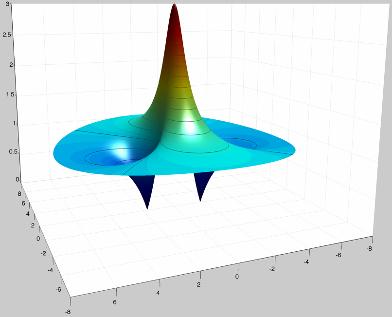
Figure 12: The theoretical shape of the spike as a function of $\displaystyle s=i\sqrt{\frac{2ibC}{y\varepsilon^{\frac{2}{5}}}}$ as given by Eq. (6-90). This also represents the exact single-breather solution $Q_{br}$ where $s=2ib(\xi+4a\eta+2ib\eta)$.

Remark 6.3

While completing the preparation of this paper we came across [1], where a hierarchy of rational breathers generalizing the standard one (6-97) is investigated. Interestingly, the maximum amplitude of these breathers is also an odd integer and hence this prompts the speculation that they should play the same rôle of (6-97) in the cases of gradient catastrophes with higher degeneracy (compare with Conjecture 6.1).

Remark 6.4 (Consistency Check)

Suppose $y$ remains fixed and $\varepsilon\to 0$ in the formulæ for $\mathbf{A},\widehat{\mathbf{A}}$ (6-74); we then obtain the limit

$$\widetilde{\Psi}_{1}(z) {\hskip-20.0pt}=F\left({\bf 1}+\left[\begin{array}[]{cc}\frac{\overline{\alpha}-\alpha}{z-\overline{\alpha}}&0\\ 0&\frac{\alpha-\overline{\alpha}}{z-\alpha}\end{array}\right]\right)\left(\frac{z-\alpha}{z-\overline{\alpha}}\right)^{-\frac{3}{4}\sigma_{3}}F^{-1}=$$ (6-104)

$${\hskip-20.0pt}=F\left[\begin{array}[]{cc}\frac{z-\alpha}{z-\overline{\alpha}}&0\\ 0&\frac{z-\overline{\alpha}}{z-\alpha}\end{array}\right]\left(\frac{z-\alpha}{z-\overline{\alpha}}\right)^{-\frac{3}{4}\sigma_{3}}F^{-1}=F\left(\frac{z-\alpha}{z-\overline{\alpha}}\right)^{\frac{1}{4}\sigma_{3}}F^{-1}=\Psi_{0}(z).$$

Figure 13: Some simple numerics (using Fast Fourier Transform) for the initial data $q(x,0)=\frac{1}{\cosh(x)}$ and $\varepsilon=\frac{1}{33}$; note that the amplitude at the first spike (numerically determined) is $|q_{peak}|=3.9256$ and $|q_{0}|=1.3137$. This is almost exactly three times, $3|q_{0}|=3.9411$. Moreover the localization of the spike at $t\simeq 0.2800$ is in excellent agreement with the theoretical value $t=0.27912...$ obtained from the numerical localization of the first pole of the tritronquée (after [24]). In this case $\mu=0$ and $t_{0}=\frac{1}{4}$ as per Example 3.1 .

Example 6.2

According to numerical studies by [24], the closest pole to the origin of the tritronquée on the bisecant of the sector where the poles are asymptotically confined is at distance of about $|v_{p}|\sim 2.38$. According to our Theorem 6.3, this is the first spike with $x=x_{p}$ after the gradient catastrophe and its location is thus determined by the map $v=v(x,t,\varepsilon)$.

In the case of the initial data of Example 3.1 with $\mu=0$, the solution is symmetric ($x\mapsto-x$), hence the first spike occurs at $x=x_{0}=0$; the time of the first spike is then estimated at

$$t_{spike}=t_{0}+\varepsilon^{\frac{4}{5}}\left(\frac{5|C_{1}|}{4}\right)^{\frac{1}{5}}\frac{1}{(2b_{0})^{\frac{3}{2}}}|v_{p}|\left(1+\mathcal{O}(\varepsilon^{\frac{2}{5}})\right).$$ (6-105)

For the case of the initial data of Example 3.1 ($\mu=0$), the exact values of $b_{0}=b(x_{0},t_{0})=\sqrt{2}$, $t_{0}=\frac{1}{4}$ and $|C_{1}|=\frac{8}{15}2^{\frac{1}{4}}$ were found in [35]; this gives

$$t_{spike}\sim\frac{1}{4}+\varepsilon^{\frac{4}{5}}0.4776312294~{}.$$ (6-106)

In Fig. 13 we report on a simple numerical example with initial data $q(x,0)=sech(x)$, $\varepsilon=\frac{1}{33}$; plotted are the profiles of $|q(x,t)|$ for $t=t_{0}=1/4$ which is the theoretical time of gradient catastrophe; the second curve is the time where numerically the maximum amplitude is achieved at $x=0$. The numerics indicates $t_{spike}=0.28$ whereas the formula (6-106) predicts $t_{spike}=0.2791260482$, which –considering that $\varepsilon$ is not that small– is an amazingly close estimate. The results on [24] do not exclude that there are closest poles to the origin: however this is the one that occurs on the same $x=x_{0}$ as the gradient catastrophe. Other numerical indications using Padé approximations localize the poles in a triangular pattern [31] like the one used as illustration in Fig. 10.

Our numerics was produced by integrating directly the NLS equation using FFT in the $x$-direction; it should be noted that the initial data we have chosen correspond to a pure soliton situation, and hence one could use a better numerical approach based on exact linear algebra as explained in [28].

Appendix A Estimate of the parametrix on a circle of large radius uniformly for large $y$

This section is rather technical; its goal is to prove that the sectorial analytic matrix function $\widehat{\Psi}(\xi;v)$, that is related to the solution $\mathbf{P}(\xi,v)$ of the RHP (4.1) through $\widehat{\Psi}(\xi;v)=G(\xi,v)\mathbf{P}(\xi,v)e^{\vartheta(\xi,v)\sigma_{3}}$, has asymptotic behavior (4-33) as $\xi\rightarrow\infty$ uniformly with respect to $v-v_{p}=O(\varepsilon^{\frac{1}{5}})$, where $v_{p}$ is one of the poles of the tritronquée solution $y(v)$ of P1, or, equivalently, uniformly with respect to $\parallel(x,t)-(x_{p},t_{p})\parallel=O(\varepsilon)$.

In fact, we will prove a somewhat stronger result, stated in Theorem A.1 below. Corollary A.1 of this theorem has been used in the main body of the paper.

Theorem A.1

Let $S$ be one of the sectors shown on Figure 9 and $\hat{\Psi}(\xi,v)=G(\xi,v)\mathbf{P}(\xi,v)e^{\vartheta(\xi,v)\sigma_{3}}$ be a solution of the ODE (4-24), obtained from the sectorial solutions $\mathbf{P}(\xi,v)$ of the Problem 4.1 in the sector $S$. Let $\Lambda$ be a constant nonsingular diagonal matrix and $\mathcal{D}_{y}$ be a disk of fixed radius $r>0$ centered at $\xi=y$. Then, there exist some constants $\xi_{*}>0$, $p_{2}>0$, both independent of $y$ and of each other, such that $\hat{\Psi}(\xi,v)$ has the representation

$$\hat{\Psi}(\xi,v)=2^{\sigma_{3}/2}(4\xi^{3}-2\xi v)^{-\sigma_{3}/4}\frac{1}{\sqrt{2}}(\sigma_{1}+\sigma_{3})T\Lambda\left({\bf 1}+O\left(\xi^{-\frac{1}{2}},{e}^{-p_{2}|\frac{y}{\xi_{*}}|^{5/2}}\right)\right)e^{\mathbf{q}(\xi,v)\sigma_{3}}$$ (A.1)

where

$${\hskip-20.0pt}\mathbf{q}(\xi,v)=\vartheta(\xi,v)+\frac{y^{\prime}}{4y}\int_{\infty}^{\xi}\frac{\left(s^{\frac{3}{2}}-\frac{v}{2\sqrt{s}}\right)ds}{(s-y)s^{2}},$$ (A.2)

$$T=\left({\bf 1}-\frac{i\sigma_{2}}{2}A_{1}\right)\left({\bf 1}-\frac{\sigma_{1}}{2}A_{2}\right) {\hskip-20.0pt}~{}~{}~{}~{}~{}{\rm with}~{}~{}~{}~{}~{}A_{1}=\frac{6\xi^{2}-v}{2(4\xi^{3}-2\xi v)^{3/2}}\ ,\qquad A_{2}=\frac{y^{\prime}\xi}{8\xi^{3}y(\xi-y)},$$ (A.3)

uniformly for $\xi\in S(\xi_{*})=S\cap\{\xi:~{}|\xi|\geq\xi_{*}\}\setminus\mathcal{D}_{y}$ and for all sufficiently large $y$. Here $\vartheta(\xi,v)=\frac{4}{5}\xi^{\frac{5}{2}}-v\sqrt{\xi}$ and the contour of integration in (A.2) is a ray in the direction of the bisector of $S$. In the case when $y\not\in S_{\xi_{*}}$ the $O$ term in (A.1) is independent of $\frac{|y|}{\xi_{*}}$, i.e., it is $O(\xi^{-\frac{1}{2}})$. The same $O$ term is valid even if $y\in S_{\xi_{*}}$ everywhere in $S_{\xi_{*}}$ except a certain“shadow” of $\mathcal{D}_{y}$ region, see Fig. 14 and description of this region below.

Proof of this theorem constitutes the bulk of this Appendix. Let us consider sector $S$ that is not adjacent to ${\mathbb{R}}_{-}$. This sector is bisected by the Stokes’ ray $\ell$ where $\Re\xi^{\frac{5}{2}}=0$. Let us extend $S$ by some angle $\delta\in(0,\frac{2}{5}\pi)$ in both directions. For definiteness, we shall focus on the sector $S=\{\arg(\xi)\in(-\delta,\frac{2\pi}{5}+\delta)\}$, the remaining being treated similarly. It is more convenient to work with variable $\vartheta(\xi,v)$ instead of $\xi$; therefore, we introduce a new variable

$$u=u(\xi)=-i\vartheta(\xi;v)=-i\left[\frac{4}{5}\xi^{5/2}-v\xi^{\frac{1}{2}}\right]~{}.$$ (A.4)

We will consider $u(\xi)$ as an analytic function (with the principal determinations of the roots) on sectors of the $\xi$–plane of width up to $4\pi/5$ and for $|\xi|$ sufficiently large: therefore in any such region the map $u(\xi)$ is holomorphically invertible because $v$ will be chosen uniformly bounded (in fact- in a neighborhood of $v_{p}$), and we will denote its inverse by $\xi(u)$. We will write for brevity $u$ or $\xi$ with the understanding that they may be viewed as functions of the other variable. A direct calculation shows that

$$\xi=\xi(u)=\left(\frac{5i}{4}\right)^{2/5}u^{2/5}\left[1+\frac{v{\rm e}^{-i\pi/5}}{5^{2/5}2^{1/5}}u^{-4/5}+O(u^{-8/5})\right],$$ (A.5)

We will let $v-v_{p}$ be bounded above, say, by $2$, and, since the branch-points of $u(\xi)$ are at $\pm\sqrt{v/2}$, the map $u(\xi)$ is invertible in any sectorial domain $\{|\xi|>|\sqrt{v}_{p}+1|$, as long as the opening of this domain is less than $2\pi$.

The image of $S$ under the map (A.4) will be denoted by $\mathfrak{S}$. Then, asymptotically for large $u$,

$$\mathfrak{S}=\{-\phi<\arg(u)<\phi\}\ ,\ \ \ \frac{1}{2}\pi<\phi<\pi.$$ (A.6)

It will be convenient for us to consider (A.6) as the definition for $\mathfrak{S}$, whereas $S$ is the preimage of $\mathfrak{S}$, i.e., $S=u^{-1}(\mathfrak{S})$. By $\mathfrak{S}_{u_{0}}$ we denote sector $\mathfrak{S}$ shifted from the origin to some $u_{0}\in{\mathbb{C}}$, i.e., $\mathfrak{S}_{u_{0}}=\mathfrak{S}+u_{0}$; for convenience we shall take $u_{0}\in{\mathbb{R}}_{+}$. Without any loss of generality we assume $u_{0}$ to be sufficiently large. Our first step in proving Theorem A.1 is to “pre-normalize” the ODE (4-24), satisfied by $\hat{\Psi}$, written with respect to the independent variable $u$.

Lemma A.1

Let $W(u)$ be defined by

$$\hat{\Psi}(\xi)=2^{\sigma_{3}/2}(4\xi^{3}-2\xi v)^{-\sigma_{3}/4}\frac{1}{\sqrt{2}}(\sigma_{1}+\sigma_{3})T(\xi)W(\xi)$$ (A.7)

where the matrix $T$ is defined by (A.3). Then $W$ satisfies the ODE in the variable $u$

$$W_{u}=\left[\left(i+\frac{iy^{\prime}\xi}{8\xi^{3}y(\xi-y)}\right)\sigma_{3}+B(u)\right]W,$$ (A.8)

where $B(u)=\mathcal{O}(u^{-6/5})$ uniformly with respect to sufficiently large values of $y$ in $u\in R_{u_{0},y}=\mathfrak{S}_{u_{0}}\setminus\Delta$. Here $\Delta=u(\mathcal{D}_{y})$.

Proof. The transformation

$$\hat{\Psi}=2^{\sigma_{3}/2}(4\xi^{3}-2\xi v)^{-\sigma_{3}/4}\frac{1}{\sqrt{2}}(\sigma_{1}+\sigma_{3})X$$ (A.9)

reduces the system (4-24) to

$$X_{\xi}=\left[\sqrt{4\xi^{3}-2\xi v}\sigma_{3}+\frac{6\xi^{2}-v}{2(4\xi^{3}-2\xi v)}\sigma_{1}+\frac{M}{2\sqrt{4\xi^{3}-2\xi v}}(\sigma_{3}+i\sigma_{2})\right]X~{},$$ (A.10)

where

$$M=2\widehat{H}_{I}+M_{2}+M_{3}=\left(2H-\frac{y^{\prime}}{y}\right)+\frac{y^{\prime}\xi}{y(\xi-y)}+\frac{3}{4(\xi-y)^{2}}.$$ (A.11)

The three terms in $M$ have uniform bounds in $S_{\xi_{0},y}=u^{-1}(R_{u_{0},y})$, where $u_{0}=u(\xi_{0})$:

• Since $\xi\not\in D$ we have $|M_{3}|<\frac{1}{r^{2}}$;

• According to (4-14) and the fact that $H^{\prime}(v)=y(v)$, we have

  $$2\widehat{H}_{I}=2H(v)-\frac{y^{\prime}(v)}{y(v)}=28\beta+O(v-v_{p});$$ (A.12)

• According to (4-14), $(\ln y)^{\prime}=-2\sqrt{y}(1+O(v-v_{p})^{4})$ for all sufficiently large $y$, so we now need to estimate $\frac{y^{\frac{1}{2}}\xi}{\xi-y}$. Note that $\left|\frac{\sqrt{\frac{y}{\xi}}}{\frac{y}{\xi}-1}\right|\leq\frac{2}{d_{0}}$ outside the domain $|\xi-y|<d_{0}|\xi|$. Thus, $M_{2}=O(\xi^{\frac{1}{2}})$ outside this domain. Inside the latter domain but outside $\mathcal{D}_{y}$ we have $\frac{y^{\frac{1}{2}}\xi}{\xi-y}=O(\xi^{\frac{3}{2}})$, so that

  $$M_{2}=O(\xi^{\frac{3}{2}})$$ (A.13)

  for all $\xi\in S_{\xi_{0},y}$ and uniformly in all sufficiently large $y$.

Rewriting (A.10) in the variable $u$ we obtain

$$X_{u}=i\frac{2\sqrt{\xi}}{4\xi^{2}-v}\left[\sqrt{4\xi^{3}-2\xi v}\sigma_{3}+\frac{6\xi^{2}-v}{2(4\xi^{3}-2\xi v)}\sigma_{1}+\frac{M}{2\sqrt{4\xi^{3}-2\xi v}}(\sigma_{3}+i\sigma_{2})\right]X=$$ (A.14)

$$=i\left[\sigma_{3}+\frac{6\xi^{2}-v}{2(4\xi^{3}-2\xi v)^{3/2}}\sigma_{1}+\frac{M}{2(4\xi^{3}-2\xi v)}(\sigma_{3}+i\sigma_{2})+\mathcal{O}(u^{-8/5})\right]X.$$ (A.15)

Dropping all the terms in $M$ except $M_{2}$, the previous equation becomes (see the bulleted list above)

$$X_{u}=i\left[\sigma_{3}+\frac{6\xi^{2}-v}{2(4\xi^{3}-2\xi v)^{3/2}}\sigma_{1}+\frac{y^{\prime}\xi(\sigma_{3}+i\sigma_{2})}{2y(\xi-y)(4\xi^{3}-2\xi v)}+\mathcal{O}(u^{-6/5})\right]X.$$ (A.16)

Using (A.13) we have

$$\frac{y^{\prime}\xi}{2y(\xi-y)(4\xi^{3}-2\xi v)}=\frac{y^{\prime}}{8y\,\xi^{2}(\xi-y)}(1+\mathcal{O}(\xi^{-2}))=\frac{y^{\prime}}{8y\,\xi^{2}(\xi-y)}+\mathcal{O}(u^{-\frac{7}{5}})$$ (A.17)

and hence

$$X_{u}=i\left[\sigma_{3}+\frac{6\xi^{2}-v}{2(4\xi^{3}-2\xi v)^{3/2}}\sigma_{1}+\frac{y^{\prime}(\sigma_{3}+i\sigma_{2})}{8\xi^{2}y(\xi-y)}+\mathcal{O}(u^{-6/5})\right]X$$ (A.18)

for $u\in R_{u_{0},y}$ uniformly in $y$ (for sufficiently large $y$). Setting $X=TW$ with $T$ as indicated in (A.3, A.7), simplifying and keeping track of the orders already estimated, yields the equation (A.8). Q.E.D.

We will use the ODE (A.8) in order to setup a recursive approximation scheme within each sector; the key is that the estimate for $B(u)$ in (A.8) is uniform for $v$ in a neighborhood of the pole $v_{p}$ (hence, for large values of $y$) and $|\xi-y|$ bounded below.

The domain $\Delta=u(D_{y})$ in the $u$ plane is of size $\mathcal{O}(|u(y)|^{\frac{3}{5}})$. For simplicity (and without real loss of generality) we modify $D$ to be the preimage of the exact disk $\Delta$ in the $u$-plane centered at $u(y)$ of the radius $d_{0}|u(y)|^{\frac{3}{5}}$.

Figure 14: Region $R_{u_{0},y}$ is the complement of $\Delta$ and the union of $\Delta^{0}$ (darker) and $R_{u_{0},y}^{0}$ (lighter). Shown in the picture are the contours of integration $\Omega_{i,j}(u)$, $u\in R_{u_{0},y}^{0}$, for the $(i,j)$ entry of the Volterra operator (A.21).

Lemma A.2

Any solution $W(u)$ to (A.8) can be written in the form $W=\Phi{\rm e}^{\mathbf{q}(u)\sigma_{3}}$ where

$$\frac{d}{du}\mathbf{q}(u)=\left(i+\frac{iy^{\prime}\xi}{8\xi^{3}y(\xi-y)}\right)$$ (A.19)

and $\Phi(u)$ solves

$$\Phi^{\prime}=\mathbf{q}^{\prime}\big{[}\sigma_{3},\Phi\big{]}+B\,\Phi$$ (A.20)

with $B=B(u)$ as in Lemma A.1 (eq. (A.8)).

Proof. A direct substitution of the proposed expression into (A.8). Q.E.D.

The differential equation (A.8) is equivalent to the following Volterra integral equation

$$\Phi(u)=\Lambda+e^{\mathbf{q}(u)}\left(\int_{\Omega(u)}e^{-\mathbf{q}(\eta)}B\Phi e^{\mathbf{q}(\eta)}d\eta\right)e^{-\mathbf{q}(u)\sigma_{3}}=\Lambda+\mathcal{I}[\Phi](u),$$ (A.21)

where $q$ from (A.19) can be written as

$$\mathbf{q}(u):=iu+\frac{iy^{\prime}}{8y}\int^{u}_{\infty}\frac{du}{(\xi(u)-y)\xi^{2}(u)}.$$ (A.22)

The symbol $\int_{\Omega(u)}$ denotes the integration along a set of contours originating at $u$ and extending to $u=\infty$, with a different direction of contour $\Omega_{i,j}(u)$ for different entries of the matrix, see Fig. 14 for the choice of the contours (the exponential of the integrand should decrease in the direction of the contour, traversed from $u$ to $\infty$). It is promptly seen from the fundamental theorem of calculus is equivalent to (A.19). The matrix $\Lambda$ is a constant of integration, which, at this point, we choose to be a diagonal and nonsingular matrix, but otherwise undetermined.

Changing variable $u=u(\xi)$ in the integral (A.22) and using $\frac{du}{d\xi}=-2i\xi^{3/2}+\frac{iv}{\sqrt{\xi}}$ and

$$\int_{\infty}^{\xi}\frac{dt}{\sqrt{t}(t-y)}=\frac{1}{\sqrt{y}}\ln\frac{\sqrt{\xi}-\sqrt{y}}{\sqrt{\xi}+\sqrt{y}},$$ (A.23)

we find

$$\mathbf{q}(u)=iu+\frac{y^{\prime}}{4y^{3/2}}\ln\frac{{\xi}-{y}}{(\sqrt{\xi}+\sqrt{y})^{2}}+O(u^{-3/5})$$ (A.24)

in the region $R_{u_{0},y}$ uniformly in $y$. Note that

$$\frac{y^{\prime}}{4y^{\frac{3}{2}}}=-\frac{1}{2}+\frac{a}{8}(v-v_{p})^{4}+\mathcal{O}((v-v_{p})^{5})=-\frac{1}{2}+\mathcal{O}(y^{-2})$$ (A.25)

and hence

$$e^{\mathbf{q}(u)\sigma_{3}}=e^{\left(\frac{4}{5}\xi^{3}-v\xi^{\frac{1}{2}}\right)\sigma_{3}}\left(\frac{\sqrt{\xi}+\sqrt{y}}{\sqrt{\xi-y}}\right)^{\sigma_{3}}({\bf 1}+O(u^{-3/5},y^{-2}))~{}$$ (A.26)

in the region $R_{u_{0},y}$ uniformly for large $y$; the cut of the logarithm is taken from $y$ to $\xi\infty$ parallel to the Stokes line (bisecant to the sector).

The strategy is to show that the integral operator $\mathcal{I}$, defined in (A.21) is contractive in a suitable space, so that a solution can be sought through an iteration scheme; the analysis depends on the region $u$ belongs to. For practical reasons we state the following lemma.

Lemma A.3

The function $\left(\frac{\sqrt{\xi}+\sqrt{y}}{\sqrt{\xi-y}}\right)$ and its inverse satisfy the inequalities

$$\left|\frac{\sqrt{\xi}\pm\sqrt{y}}{\sqrt{\xi-y}}\right|\leq K_{0}|\xi|^{\frac{1}{2}}$$ (A.27)

outside the circle $|\xi-y|\geq r$, with $K_{0}$ a constant independent of $y$ (but depending on $r$).

Proof. The function $\left(\frac{\sqrt{\xi}+\sqrt{y}}{\sqrt{\xi-y}}\right)$ is continuous (in fact smooth except at $\xi=0$ and $\xi=y$) on ${\mathbb{C}}\setminus\{y\}$ and has limit $1$ at $\xi=\infty$, being unbounded in any neighborhood of $\xi=y$. It can be also seen by calculus that it has no critical values in ${\mathbb{C}}\setminus\{0,y\}$ and hence the maximum is attained on a disk around $y$. The value there is easily estimated as in (A.27). Similar arguments work for the inverse function. Q.E.D.

A.1 Convergence of iterations in $R_{u_{0},y}^{0}$

The region $R_{u_{0},y}^{0}$ is the lighter shaded region in Fig. 14; it is obtained by excising from $R_{u_{0},y}$ the “cone of shadow” of the disk $\Delta$ with the angle $\phi_{2}\in(\phi,\pi)$ indicated in Fig. 14 chosen arbitrarily and fixed once and for all. The region $\Delta^{0}$ will be such cone of shadow. For a given $u\in R^{0}_{u_{0},y}$, the contours of integration $\Omega_{i,j}(u)$ are also shown in Fig. 14. It is important that the collection of contours $\Omega(u)\subset R_{u_{0},y}^{0}$ for any $u\in R_{u_{0},y}^{0}$.

Lemma A.4

If a matrix-function $\chi(u)$ satisfies $\|\chi(u)\|\leq c|u|^{-m}$ in $R^{0}_{u_{0},y}$ for some $c>0$ and some $m\geq 0$ then $\|\mathcal{I}_{1}\chi(u)\|\leq cK_{1}|u|^{-m-1/5}$, where $\mathcal{I}_{1}$ denoted the Volterra integral operator (A.21) with the contours $\Omega(u)$ specified above. The constant $K_{1}$ does not depend on $\chi$, $u_{0}\in{\mathbb{R}}^{+}$ and $y\in{\mathbb{C}}$, but depend on $m$ (it was assumed above that $u_{0}$ and $|y|$ are large).

Proof. The diagonal entries of $B\chi$ are unaffected by the conjugation by ${\rm e}^{\mathbf{q}\sigma_{3}}$ and are of order $u^{-m-\frac{6}{5}}$: after integration they become of order $u^{-m-\frac{1}{5}}$. Regarding the off–diagonal entries of $B\chi$, let $F(u)$ denote one of them; then, according to (A.21), $|F(u)|\leq cL|u|^{-m-\frac{6}{5}}$ on $R_{u_{0},y}$, where the constants $L>0$ and $m\geq 0$ do not depend on $y$ and we have (from (A.26))

$${\rm e}^{\pm 2\mathbf{q}(u)}F(u)={\rm e}^{\pm 2iu}F(u)\left(\frac{\sqrt{\xi}+\sqrt{y}}{\sqrt{\xi-y}}\right)^{2}({\bf 1}+O(u^{-3/5},y^{-2})),$$ (A.28)

so that

$$\left|F(u)\left(\frac{\sqrt{\xi}+\sqrt{y}}{\sqrt{\xi-y}}\right)({\bf 1}+O(u^{-3/5},y^{-2}))\right|\leq cLK_{0}\sqrt{|\xi|}|u|^{-m}=cLK_{0}|u|^{-m-1}.$$ (A.29)

Due to the choice of the contours $\Omega(u)$, the integration along the corresponding $\Omega_{i,j}(u)$ can change the previous estimate only by a constant that does not depend on $u_{0}$ and $y$ (but depends on $\phi_{2}$). Q.E.D.

Let us consider successive iterations $\Phi_{n}=\mathcal{I}_{1}\Phi_{n-1}$, $n\geq 1$, of equation (A.21), where $\Phi_{0}=0$. Let $\Delta\Phi_{n}=\Phi_{n}-\Phi_{n-1}$. Then $\Phi_{1}=\Delta\Phi_{1}=\Lambda$ and $\Delta\Phi_{n}=\mathcal{I}_{1}\Delta\Phi_{n-1}$. We are now going to prove uniform in $y$ convergence of the series $\sum_{1}^{\infty}\Delta\Phi_{n}$ in different subregions of $R_{u_{0},y}$, provided that $u_{0}$, which is independent of $y$, is large enough. In all the analysis below $y$ is assumed to be large.

Let $\|\Lambda\|=c$. Then, according to Lemma A.4, $\|\Delta\Phi_{2}\|\leq cK_{1}|u|^{-1/5}$ in $R^{0}_{u_{0},y}$ uniformly in $u_{0}$ and in $y$. We can choose $u_{0}\in{\mathbb{R}}^{+}$ so large that $K_{1}|u|^{-1/5}<\frac{1}{2}$ for all $u\in R^{0}_{u_{0},y}$. This choice of $u_{0}$ guarantees convergence of the series $\sum_{1}^{\infty}\Delta\Phi_{n}$ in $R^{0}_{u_{0},y}$ uniformly in $y$. Moreover, we obtain the estimate

$$\Phi(u)=\Lambda[{\bf 1}+O(u^{-1/5})]$$ (A.30)

in $R^{0}_{u_{0},y}$ uniformly in $y$.

Let $\mathcal{R}_{\xi_{0},y}$ denote the preimage of $R^{0}_{u_{0},y}$ under the map $u=u(\xi)$, where $u_{0}=u(\xi_{0})$. Going back to the system (4-24), we obtain the following result.

Lemma A.5

The solution $\hat{\Psi}(\xi,v)$ to the system (4-24) has behavior

$$\hat{\Psi}(\xi,v)=2^{\sigma_{3}/2}(4\xi^{3}-2\xi v)^{-\sigma_{3}/4}\frac{1}{\sqrt{2}}(\sigma_{1}+\sigma_{3})T\Lambda({\bf 1}+O(\xi^{-\frac{1}{2}}))e^{\mathbf{q}(u(\xi))}$$ (A.31)

in $\mathcal{R}_{\xi_{0},y}$ uniformly in $y$ provided $\xi_{0}$ is large enough. Moreover, for a fixed diagonal $\Lambda$, condition (A.31) uniquely determines the solution $\hat{\Psi}(\xi,v)$ of (4-24).

Comparison of (A.31) and (4-18) together with the asymptotics of $\Psi$ (4-13) and (4-30) yields

$$\Lambda={\rm diag}(1,i).$$ (A.32)

A.2 Convergence of iterations in $\Delta^{0}$

If $y$ does not belong to the sector $S$ we are considering, we can always arrange that $\mathcal{D}_{y}\cap S=\emptyset$, so that $\mathcal{R}_{\xi_{0},y}$ coincides with the preimage of $\mathfrak{S}_{u_{0}}$ and, thus, the estimate of Lemma A.5 holds throughout that sector. We want to extend the statement of Lemma A.5 into the preimage $\mathcal{D}^{0}$ of the region $\Delta^{0}$ for the case that $y\in S$. Because of the construction of $S$ we can assume, without any loss of generality, that $y\in\widehat{S}$, where $\widehat{S}$ is any proper subsector of $S$.

Consider the tangent line $\lambda$ to the disk $\Delta$ (which is centered at $u(y)$) that is parallel to $e^{-i\phi_{1}}$ and located above $\Delta$, i.e., if $u_{*}$ is the point of tangency, then $\arg u_{*}>\arg u(y)$. Here $\phi_{1}\in(\phi,\phi_{2})$. It is clear that $\lambda$ divides $\mathfrak{S}_{u_{0}}$ into two regions. Let $R^{1}_{u_{0},y}$ denote one of these regions, namely, the one that does not contain $\Delta$. We want to extend the statement of Lemma A.5 into the region $R^{1}_{u_{0},y}$. To this end, we construct a solution $\tilde{\Phi}$ of the integral equation (A.21) in $R^{1}_{u_{0},y}$ by successive iterations. Let $u_{1}$ denote the point of intersection of $\partial\mathfrak{S}_{u_{0}}$ and $\lambda$. The collection of contours of integration $\Omega(u)$ in the case of the region $R^{1}_{u_{0},y}$ is similar to the case of the region $R^{0}_{u_{0},y}$, considered above, except that the contour of integration for the entry $(1,2)$ is the segment $[u_{1},u]$, provided that $[u_{1},u]\subset R^{1}_{u_{0},y}$. For $u\in R^{1}_{u_{0},y}$ that do not satisfy the latter condition, the contour of integration is the union of $[u_{1},u_{0}]\cup[u_{0},u]$.

Let $\mathcal{I}_{2}$ denote the integral operator in the Volterra equation (A.21) in the region $R^{1}_{u_{0},y}$ with the contours defined above. We can repeat the previous estimates of integrals to extend the statement of Lemma A.4 to the integral operator $\mathcal{I}_{2}$ in the region $R^{1}_{u_{0},y}$: the only difference is the finite contour of integration, where the desired estimate comes from Lemma 14.2, [38]. The solution $\tilde{\Phi}$ to (A.21) thus satisfies the same estimate of Lemma A.5. We also have

$$\tilde{\Phi}(u)=\Lambda\left({\bf 1}+O(u^{-1/5})\right)$$ (A.33)

in $R^{1}_{u_{0},y}$ uniformly in $y$. Here $\Lambda$ is given by (A.32).

Let $u_{0}\in{\mathbb{R}}_{+}$ be fixed: for any sufficiently large $|u(y)|$ the set $R^{0}_{u_{0},y}\cap R^{1}_{u_{0},y}$ consists of two disjoint components $\Upsilon^{1,2}_{u_{0},y}$ shown in Fig. 15 (otherwise, we can extend $\Delta$ in such a way that it will intersect the boundary of $\mathfrak{S}_{u_{0}}$ and the corresponding $\Delta^{0}$ disappear). Let $S(y)$ denote the Stokes matrix connecting solutions of (A.8) $\tilde{\Phi}{\rm e}^{\mathbf{q}\sigma_{3}}$ and the previously constructed one $\Phi{\rm e}^{\mathbf{q}\sigma_{3}}$. Then

$$\Phi(u,y)=\tilde{\Phi}(u,y)e^{\mathbf{q}(u,y)\sigma_{3}}S(y)e^{-\mathbf{q}(u,y)\sigma_{3}},\qquad S(y)=\left(\begin{array}[]{cc}1&s(y)\\ 0&1\end{array}\right),$$ (A.34)

where the triangularity of $S(y)$ follows from the fact that $\Phi,\tilde{\Phi}\to\Lambda$ as $u\rightarrow\infty$, $u\in\Upsilon^{2}_{u_{0},y}$. Writing $\mathbf{q}=\mathbf{q}(u,y)$ in (A.34), we emphasize that $\mathbf{q}$ depends on $y$.

Estimate for $\mathbf{s(y)}$.

We now want to obtain an estimate for $s(y)$ by comparing $\Phi$ and $\tilde{\Phi}$ in the region $\Upsilon_{u_{0},y}^{1}$. Let us denote by $\widehat{\Phi}$ the analytic continuation of $\Phi$ from $\Upsilon^{2}_{u_{0},y}$ throughout $R^{1}_{u_{0},y}$ (throughout the dark shaded region) into $\Upsilon^{1}_{u_{0},y}$. According to (4-18), $\hat{\Psi}(\xi,y)$ has monodromy $-{\bf 1}$ as $\xi$ goes around $\xi=y$. Because of (A.7), $W=\Phi\,{\rm e}^{\mathbf{q}\sigma_{3}}$ has the same monodromy. It follows from (A.24) that ${\rm e}^{\mathbf{q}\sigma_{3}}$ has monodromy $Mm_{y}:=\exp\left[2i\pi\frac{y^{\prime}}{4y^{\frac{3}{2}}}\sigma_{3}\right]$ around $\xi=y$. Therefore we have

$$\widehat{\Phi}(u;y)=-\Phi(u;y)m_{y}^{-1}\ ,\qquad u\in\Upsilon_{u_{0},y}^{1}.$$ (A.35)

The matrix $m_{y}$ (which is constant in $u$!) has the behavior $m_{y}=-{\bf 1}+\mathcal{O}(y^{-2})$ on account of (A.25). According to (A.30 and the fact that $m_{y}$ is uniformly bounded (for all large $y$), we have

$$\|\widehat{\Phi}-\Lambda\|\leq K_{2}|u|^{-\frac{1}{5}},~{}~{}\|\Phi-\Lambda\|\leq K_{2}|u|^{-\frac{1}{5}}\ \hbox{ in }\Upsilon^{1}_{u_{0},y},$$ (A.36)

with a constant $K_{2}$ independent of $y$. But, according to (A.33), $\widetilde{\Phi}$ too satisfies the same estimate. Substituting these estimates into (A.34), we obtain

$$s(y){\rm e}^{2\mathbf{q}(u)}=O(u^{-\frac{1}{5}})$$ (A.37)

in $\Upsilon^{1}_{u_{0},y}$ uniformly in $y$. In particular, according to (A.24), $|s(y)|\leq K_{3}|u_{1}|^{\frac{1}{5}}e^{2\Im u_{1}}$ for some $K_{3}>0$ that is independent of $y$. Therefore, in the region $\Delta^{0}\cup R^{1}_{u_{0},y}$ (darker shade on Fig. 15), we have

$$\left|s(y){\rm e}^{2\mathbf{q}(u)}\right|\leq K_{3}|u_{1}|^{\frac{1}{5}}e^{2\Im(u_{1}-u)}$$ (A.38)

Given the geometry of regions and the fact that $y\in\widehat{S}$, we have

$$\Im(u-u_{1})\geq K_{4}|u(y)-u_{1}|\geq K_{5}|u(y)-u_{0}|,\ \ \forall u\in\Delta^{0},$$ (A.39)

where $K_{4},K_{5}$ denote some positive constants independent of $u_{0},y$. Thus, the matrix $e^{\mathbf{q}(u,y)\sigma_{3}}S(y)e^{-\mathbf{q}(u,y)\sigma_{3}}$ in (A.34) is exponentially close to ${\bf 1}$ as $y-\xi_{0}\rightarrow\infty$, where $u(\xi_{0})=u_{0}$. So, according to (A.34), the estimate of Lemma A.5 (with a modified $O$ term) can be extended to $\Delta^{0}$ (more precisely, to the shaded part of it $\Delta^{0}\cap R^{1}_{u_{0},y}$), provided $y-\xi_{0}\rightarrow\infty$. Because of the construction of $\widehat{S}$, there exists $\mu>0$, such that $\widehat{S}$ contains $S(\mu|\xi_{0}|)$, where by $S$ now we mean the original sector of the RHP (9), see Theorem (A.1). We denote $\xi_{*}=\mu|\xi_{0}|$. Existence of the positive constant $p_{2}$ in the estimate (A.1) follows from (A.34) (A.38) and (A.39). The case of sectors $S$ adjacent to the jump contour ${\mathbb{R}}_{-}$ on Fig. 9 can be considered similarly since we can rotate this contour in both directions by angle up to $\frac{\pi}{5}$.

The proof of Theorem A.1 is completed.

Figure 15: The region $R^{1}_{u_{0},y}$ (shaded) and its two subregions $\Upsilon^{1}_{u_{0},y}$, $\Upsilon^{2}_{u_{0},y}$ (lighter shading). The goal is to extend the estimate (A.31) into the remaining third (darker shading) subregion of $R^{1}_{u_{0},y}$.

According to (A.3) and (A.13), the matrix $T$ from (A.1) can be absorbed into ${\bf 1}+O(\xi^{-\frac{1}{2}})$ term. To within the same estimate we can replace also $\sqrt{4\xi^{3}-v\xi}$ by $2\xi^{\frac{3}{2}}$ and recast the theorem into

Corollary A.1

Under the same assumptions and in the same notations of Theorem A.1 we have

$$\hat{\Psi}(\xi,v)=\xi^{-\frac{3}{4}\sigma_{3}}\frac{1}{\sqrt{2}}(\sigma_{1}+\sigma_{3})\left(\Lambda+O\left(\xi^{-\frac{1}{2}},y^{-4},{e}^{-p_{2}|\frac{y}{\xi_{*}}|^{5/2}}\right)\right)\left(\frac{\sqrt{\xi}+\sqrt{y}}{\sqrt{\xi-y}}\right)^{\sigma_{3}}{\rm e}^{\vartheta(\xi;v)\sigma_{3}}$$ (A.40)

with the understanding that $|\xi|\to\infty$ and $|y|\to\infty$ and $|\xi-y|$ is bounded uniformly away from zero.

Theorem A.1 together with the convergence of iterations imply the following corollary.

Corollary A.2

For any sufficiently large $\xi$ we have $\lim_{v\rightarrow v_{p}}\hat{\Psi}(\xi,v)=\hat{\Psi}(\xi,v_{p})$.

Acknowledgments.

The authors are grateful to Percy Deift and to Peter Miller for useful discussions. A. T. thanks the hospitality and support of the Mathematical Physics Laboratory at the Centre de recherches mathématiques where part of the work was carried out. M. B. was supported by the NSERC Discovery Grant ”Exact and asymptotic methods in Random Matrix Theory and Integrable Systems”.

References

• [1] A. Ankiewicz, P. A. Clarkson, and Nail Akhmediev. Rogue waves, rational solutions, the patterns of their zeros and integral relations. J. Phys. A: Math. Theor., 43(12), 2010.
• [2] V. I. Arnol’d, S. M. Guseĭn-Zade, and A. N. Varchenko. Singularities of differentiable maps. Vol. I, volume 82 of Monographs in Mathematics. Birkhäuser Boston Inc., Boston, MA, 1985. The classification of critical points, caustics and wave fronts, Translated from the Russian by Ian Porteous and Mark Reynolds.
• [3] R.  J. Buckingham and P. D. Miller. The sine-Gordon equation in the semiclassical limit: critical behavior near a separatrix. Journal d’Analyse Mathématique, to appear.
• [4] M. Bertola and S. Y. Lee. First colonization of a spectral outpost in random matrix theory. Constr. Approx., 30(2):225–263, 2009.
• [5] M Bertola and A. Tovbis. Universality in the profile of the semiclassical limit solutions to the focusing nonlinear schrödinger equation at the first breaking curve. Int. Math. Res. Not., 2009.
• [6] P. Bleher and A. Its. Double scaling limit in the random matrix model: the Riemann-Hilbert approach. Comm. Pure Appl. Math., 56(4):433–516, 2003.
• [7] P. Boutroux. Recherches sur les transcendantes de M. Painlevé et l’étude asymptotique des équations différentielles du second ordre. Ann. Sci. École Norm. Sup. (3), 30:255–375, 1913.
• [8] P. Boutroux. Recherches sur les transcendantes de M. Painlevé et l’étude asymptotique des équations différentielles du second ordre (suite). Ann. Sci. École Norm. Sup. (3), 31:99–159, 1914.
• [9] D. Cai, D. W. McLaughlin, and K. T. R. McLaughlin. The nonlinear Schrödinger equation as both a PDE and a dynamical system. In Handbook of dynamical systems, Vol. 2, pages 599–675. North-Holland, Amsterdam, 2002.
• [10] T. Claeys and T. Grava. Universality of the break-up profile for the KdV equation in the small dispersion limit using the Riemann-Hilbert approach. Comm. Math. Phys., 286(3):979–1009, 2009.
• [11] T. Claeys and M. Vanlessen. Universality of a double scaling limit near singular edge points in random matrix models. Comm. Math. Phys., 273(2):499–532, 2007.
• [12] P. Deift, T. Kriecherbauer, K. T.-R. McLaughlin, S. Venakides, and X. Zhou. Uniform asymptotics for polynomials orthogonal with respect to varying exponential weights and applications to universality questions in random matrix theory. Comm. Pure Appl. Math., 52(11):1335–1425, 1999.
• [13] P. Deift and X. Zhou. A steepest descent method for oscillatory Riemann-Hilbert problems. Bull. Amer. Math. Soc. (N.S.), 26(1):119–123, 1992.
• [14] J. DiFranco, P. D. Miller and B. Muite. On the modified nonlinear Schrödinger equation in the semiclassical limit: supersonic, subsonic, and transsonic behavior. Acta Math. Sci., 31 : 2343-2377, 2011.
• [15] B. Dubrovin, T. Grava, and C. Klein. On universality of critical behavior in the focusing nonlinear Schrödinger equation, elliptic umbilic catastrophe and the tritronquée solution to the Painlevé-I equation. J. Nonlinear Sci., 19(1):57–94, 2009.
• [16] M. Duits and and A.B.J. Kuijlaars, Painlevé I asymptotics for orthogonal polynomials with respect to a varying quartic weight. Nonlinearity 19:2211–2245, 2006.
• [17] A.S. Fokas, A.R. Its, and A.V. Kitaev, The isomonodromy approach to matrix models in 2D quantum gravity. Comm. Math. Phys., 147 (1992), 395–430.
• [18] A. S. Fokas, A. R. Its, A. A. Kapaev, and V. Yu. Novokshenov. Painlevé transcendents, volume 128 of Mathematical Surveys and Monographs. American Mathematical Society, Providence, RI, 2006. The Riemann-Hilbert approach.
• [19] M. G. Forest and J. E. Lee. Geometry and modulation theory for the periodic nonlinear Schrödinger equation. In Oscillation theory, computation, and methods of compensated compactness (Minneapolis, Minn., 1985), volume 2 of IMA Vol. Math. Appl., pages 35–69. Springer, New York, 1986.
• [20] R. Jenkins and K.  D.  T.-R. McLaughlin. The semiclassical limit of focusing NLS for a family of non-analytic initial data. arXiv:1106.1699, 72p.
• [21] M. Jimbo and T. Miwa. Monodromy preserving deformation of linear ordinary differential equations with rational coefficients. II. Phys. D, 2(3):407–448, 1981.
• [22] M. Jimbo and T. Miwa. Monodromy preserving deformation of linear ordinary differential equations with rational coefficients. III. Phys. D, 4(1):26–46, 1981/82.
• [23] M. Jimbo, T. Miwa, and K. Ueno. Monodromy preserving deformation of linear ordinary differential equations with rational coefficients. I. General theory and $\tau$-function. Phys. D, 2(2):306–352, 1981.
• [24] N. Joshi and A. V. Kitaev. On Boutroux’s tritronquée solutions of the first Painlevé equation. Stud. Appl. Math., 107(3):253–291, 2001.
• [25] S. Kamvissis, K. D. T.-R. McLaughlin, and P. D. Miller. Semiclassical soliton ensembles for the focusing nonlinear Schrödinger equation, volume 154 of Annals of Mathematics Studies. Princeton University Press, Princeton, NJ, 2003.
• [26] A. A. Kapaev. Quasi-linear stokes phenomenon for the Painlevé first equation. J. Phys. A, 37(46):11149–11167, 2004.
• [27] P.  D. Lax and C.  D. Levermore, The small dispersion limit of the Korteweg-de Vries equation. Part I. Comm. Pure Appl. Math. 36(3): 253-290, 1983. Part II. Comm. Pure Appl. Math. 36(5): 571-593, 1983.
• [28] G. D. Lyng and P. D. Miller. The $N$-soliton of the focusing nonlinear Schrödinger equation for $N$ large. Comm. Pure Appl. Math., 60(7):951–1026, 2007.
• [29] D. Masoero. Poles of intégrale tritronquée and anharmonic oscillators. A WKB approach. J. Phys. A: Math. Theor., 43(095201), 09 2010.
• [30] P. D. Miller and S. Kamvissis. On the semiclassical limit of the focusing nonlinear Schrödinger equation. Phys. Lett. A, 247(1-2):75–86, 1998.
• [31] V. Yu. Novokshenov. Poles of tritronquée solution to the Painlevé I equation and cubic anharmonic oscillator. Regul. Chaotic Dyn., 15(2-3):390–403, 2010. see also the Erratum on Regul. Chaotic Dyn. 15(6):717, 2010.
• [32] D. H. Peregrine. Water waves, nonlinear Schrödinger equations and their solutions. J. Austral. Math. Soc. Ser. B, 25(1):16–43, 1983.
• [33] A. Tovbis and M. Hoefer, Semiclassical dynamics of quasi-one-dimensional, attractive Bose-Einstein condensates. Phys. Lett. A 375(3): 726-732, 2011.
• [34] A. Tovbis and S. Venakides. Semiclassical limit of the scattering transform for the focusing nonlinear schrödinger equation. IMRN, doi: 10.1093/imrn/rnr092, 60p., 2011.
• [35] A. Tovbis, S. Venakides, and X. Zhou. On semiclassical (zero dispersion limit) solutions of the focusing nonlinear Schrödinger equation. Comm. Pure Appl. Math., 57(7):877–985, 2004.
• [36] A. Tovbis, S. Venakides, and X. Zhou. Semiclassical focusing nonlinear Schrödinger equation I: inverse scattering map and its evolution for radiative initial data. Int. Math. Res. Not. IMRN, (22):Art. ID rnm094, 54, 2007.
• [37] E. R. Tracy and H. H. Chen. Nonlinear self-modulation: an exactly solvable model. Phys. Rev. A (3), 37(3):815–839, 1988.
• [38] W. Wasow. Asymptotic expansions for ordinary differential equations. Dover Publications Inc., New York, 1987. Reprint of the 1976 edition.
• [39] V. E. Zaharov and A. B. Šabat. Integration of the nonlinear equations of mathematical physics by the method of the inverse scattering problem. II. Funktsional. Anal. i Prilozhen., 13(3):13–22, 1979.
• [40] X. Zhou, The $L^{2}$-Sobolev space bijectivity of the scattering and inverse scattering transforms. Comm. Pure Appl. Math., 51:697–731, 1998.
• [41] X. Zhou, Zakharov-Shabat inverse scattering. In Scattering and inverse scattering in pure and applied science, pages 1707–1716. Academic Press, London, 2002.