Phase Transitions for Greedy Sparse Approximation Algorithms

Abstract

A major enterprise in compressed sensing and sparse approximation is the design and analysis of computationally tractable algorithms for recovering sparse, exact or approximate, solutions of underdetermined linear systems of equations. Many such algorithms have now been proven to have optimal-order uniform recovery guarantees using the ubiquitous Restricted Isometry Property (RIP) [10]. However, it is unclear when the RIP-based sufficient conditions on the algorithm are satisfied. We present a framework in which this task can be achieved; translating these conditions for Gaussian measurement matrices into requirements on the signal’s sparsity level, length, and number of measurements. We illustrate this approach on three of the state-of-the-art greedy algorithms: CoSaMP [29], Subspace Pursuit (SP) [12] and Iterative Hard Thresholding (IHT) [7]. Designed to allow a direct comparison of existing theory, our framework implies that, according to the best known bounds, IHT requires the fewest number of compressed sensing measurements and has the lowest per iteration computational cost of the three algorithms compared here.

1 Introduction

In compressed sensing [9, 10, 17], one works under the sparse approximation assumption, namely, that signals/vectors of interest can be well approximated by few components of a known basis. This assumption is often satisfied due to constraints imposed by the system which generates the signal. In this setting, it has been proven (originally in [10, 17] and by many others since) that the number of linear observations of the signal, required to guarantee recovery, need only be proportional to the sparsity of the signal’s approximation. This is in stark contrast to the standard Shannon-Nyquist Sampling paradigm [36] where worst-case sampling requirements are imposed.

In the simplest setting, consider measuring a vector $x_{0}\in\mathbb{R}^{N}$ which either has exactly $k<N$ nonzero entries, or which has $k$ entries whose magnitudes are dominant. Let $A$ be an $n\times N$ matrix with $n<N$ which we use to measure $x_{0}$; the $n$ inner products with $x_{0}$ are the entries in $y=Ax_{0}$. From knowledge of $y$ and $A$ one seeks to recover the vector $x_{0}$, or a suitable approximation thereof, [8]. Let $\chi^{N}(k):=\left\{x\in\mathbb{R}^{n}:\left\|x\right\|_{0}\leq k\right\}$ denote the family of at most $k$-sparse vectors in $\mathbb{R}^{N}$, where $\left\|\cdot\right\|_{0}$ counts the number of nonzero entries. From $y$ and $A$, the optimal $k$-sparse signal is the solution of

$$\min_{x\in\chi^{N}(k)}\left\|Ax-y\right\|_{2},$$ (1)

where $\|\cdot\|_{2}$ denotes the Euclidean norm.

However, solving (1) via a naive exhaustive search is combinatorial in nature and NP-hard [28]. A major aspect of compressed sensing theory is the study of alternative methods to solving (1). Since the system $y=Ax$ is underdetermined, any successful recovery of $x$ will require some form of nonlinear reconstruction. Under certain conditions, various algorithms have been shown to successfully reduce (1) to a tractable problem, one with a computational cost which is a low degree polynomial of the problem dimensions, rather than the exponential cost associated with a direct combinatorial search for the solution of (1). While there are numerous reconstruction algorithms, they each generally fall into one of three categories: greedy methods, regularizations, or combinatorial group testing. For an indepth discussion of compressed sensing recovery algorithms, see [29] and references therein.

The first uniform guarantees for exact reconstruction of every $x\in\chi^{N}(k)$, for a fixed $A$, came from $\ell_{1}$-regularization. In this case, (1) is relaxed to solving the problem

$$\min_{x\in\mathbb{R}^{N}}\left\|x\right\|_{1}\ \hbox{subject to}\ \left\|Ax-y\right\|_{2}<\gamma,$$ (2)

for some known noise level, or decreasing, $\gamma$. $\ell_{1}$-regularization has been extensively studied, see the pioneering works [10, 17]; also, see [16, 21, 6] for results analogous to those presented here. In this paper, we focus on three illustrative greedy algorithms, Compressed Sensing Matching Pursuit (CoSaMP) [29], Subspace Pursuit (SP) [12], and Iterative Hard Thresholding (IHT) [7], which boast similar uniform guarantees of successful recovery of sparse signals when the measurement matrix $A$ satisfies the now ubiquitous Restricted Isometry Property (RIP) [10, 6]. The three algorithms are deeply connected and each have some advantage over the other. These algorithms are essentially support set recovery algorithms which use hard thresholding to iteratively update the approximate support set; their differences lie in the magnitude of the application of hard thresholding and the vectors to which the thresholding is applied, [14, 37]. The algorithms are restated in the next section. Other greedy methods with similar guarantees are available, see for example [11, 27]; several other greedy techniques have been developed ([23, 30, 13], etc.), but their theoretical analyses do not currently subscribe to the above uniform framework.

As briefly mentioned earlier, the intriguing aspect of compressed sensing is its ability to recover $k$-sparse signals when the number of measurements required is proportional to the sparsity, $n\sim k$, as the problem size grows, $n\rightarrow\infty$. Each of the algorithms discussed here exhibit a phase transition property, where there exists a $k_{n}^{\ast}$ such that for any $\epsilon>0$, as $k_{n}^{\ast},n\rightarrow\infty$, the algorithm successfully recovers all $k$-sparse vectors provided $k<(1-\epsilon)k^{\ast}_{n}$ and does not recover all $k$-sparse vectors if $k>(1+\epsilon)k_{n}^{\ast}$. For a description of phase transitions in the context of compressed sensing, see [15], while for numerical average-case phase transitions for greedy algorithms, see [14]. We consider the asymptotic setting where $k$ and $N$ grow proportionally with $n$, namely, $(k,n,N)\rightarrow\infty$ with the ratios $\frac{k}{n}\rightarrow\rho,\frac{n}{N}\rightarrow\delta$ as $n\rightarrow\infty$ for $(\delta,\rho)\in(0,1)^{2}$; also, we assume the matrix $A$ is drawn i.i.d. from $\mathcal{N}(0,n^{-1})$, the normal distribution with mean $0$ and variance $n^{-1}$. In this framework, we develop lower bounds on the phase transition for exact recovery of all $k$-sparse signals. These bounds provide curves in the unit square, $(\delta,\rho)\in(0,1)^{2}$, below which there is an exponentially high probability on the draw the Gaussian matrix $A$, that $A$ will satisfy the sufficient RIP conditions and therefore solve (1). We utilize a more general, asymmetric version of the RIP, see Definition 1, to compute as precise a lower bound on the phase transitions as possible. This phase transition framework allows a direct comparison of the provable recovery regions of different algorithms in terms of the problem instance $(\frac{n}{N},\frac{k}{n})$ . We then compare the guaranteed recovery capabilities of these algorithms to the guarantees of $\ell_{1}$-regularization proven via RIP analysis. For $\ell_{1}$-regularization, this phase transition framework has already been applied using the RIP [5, 6], using the theory of convex polytopes [16] and geometric functional analysis [35].

The aforementioned lower bounds on the algorithmic exact sparse recovery phase transitions are presented in Theorems 10, 11, and 12. The curves are defined by functions $\rho_{S}^{sp}(\delta)$ (SP; the magenta curve in Fig.1(a)), $\rho_{S}^{csp}(\delta)$ (CoSaMP; the black curve in Fig.1(a)), $\rho_{S}^{iht}(\delta)$ (IHT; the red curve in Fig.1(a)). For comparison, the analogous lower bound on the phase transition for $\rho_{S}^{\ell_{1}}(\delta)$ ($\ell_{1}$-regularization) is displayed as the blue curve in Fig.1(a). From Fig. 1, we are able to directly compare the provable recovery results of the three greedy algorithms as well as $\ell_{1}$-regularization. For a given problem instance $(k,n,N)$ with the entries of $A$ drawn i.i.d. from $\mathcal{N}(0,n^{-1})$, if $\frac{k}{n}=\rho$ falls in the region below the curve $\rho_{S}^{alg}(\delta)$ associated to a specific algorithm, then with probability approaching 1 exponentially in $n$, the algorithm will exactly recover the $k$-sparse vector $x\in\chi^{N}(k)$ no matter which $x\in\chi^{N}(k)$ was measured by $A$. These lower bounds on the phase transition can also be interpreted as the minimum number of measurements known to guarantee recovery through the constant of proportionality: $n>\left(\rho_{S}^{alg}\right)^{-1}k$. Fig. 1(b) portrays the inverse of the lower bounds on the phase transition. This gives a minimum possible value for $\left(\rho_{S}^{alg}\right)^{-1}$. For example, from the blue curve, for a Gaussian random matrix used in $\ell_{1}$-regularization, the minimum number of measurements proven (using RIP) to be sufficient to ensure recovery of all $k$-sparse vectors is $n>317k$. By contrast, for greedy algorithms, the minimum number of measurements shown to be sufficient is significantly larger: $n>907k$ for IHT, $n>3124k$ for SP, and $n>4923k$ for CoSaMP.

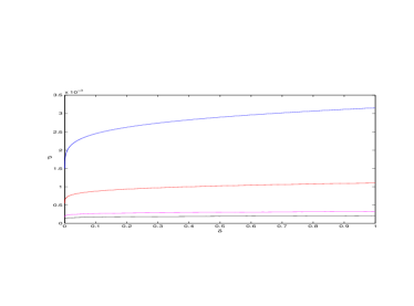
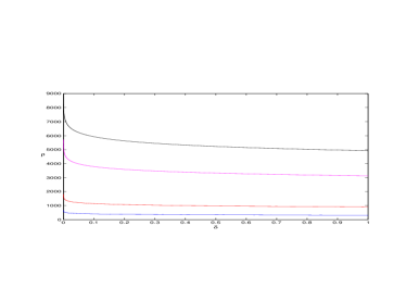
(a)	(b)

Figure 1: (a): The lower bounds on the Strong exact recovery phase transition for Gaussian random matrices for the algorithms $\ell_{1}$-regularization (Theorem 13, $\rho_{S}^{\ell_{1}}(\delta)$, blue), IHT (Theorem 12, $\rho_{S}^{iht}(\delta)$, red), SP (Theorem 11, $\rho_{S}^{sp}(\delta)$, magenta), and CoSaMP (Theorem 10, $\rho_{S}^{csp}(\delta)$, black). (b): The inverse of the phase transition lower bounds in the left panel (a).

More precisely, the main contributions of this article is the derivation of theorems and corollaries of the following form for each of the CoSaMP, SP, and IHT algorithms.

Theorem 1

Given a matrix $A$ with entries drawn i.i.d. from ${\cal N}(0,n^{-1})$, for any $x\in\chi^{N}(k)$, let $y=Ax+e$ for some (unknown) noise vector $e$. For any $\epsilon\in(0,1)$, as $(k,n,N)\rightarrow\infty$ with $n/N\rightarrow\delta\in(0,1)$ and $k/n\rightarrow\rho\in(0,1)$, there exists $\mu^{alg}(\delta,\rho)$ and $\rho_{S}^{alg}(\delta)$, the unique solution to $\mu^{alg}(\delta,\rho)=1$. If $\rho<(1-\epsilon)\rho_{S}^{alg}(\delta)$, there is an exponentially high probability on the draw of $A$ that the output of the algorithm at the $l^{th}$ iteration, $\hat{x}$, approximates $x$ within the bound

$$\|x-\hat{x}\|_{2}\leq\kappa^{alg}(\delta,(1+\epsilon)\rho)\left[\mu^{alg}(\delta,(1+\epsilon)\rho)\right]^{l}\|x\|_{2}+\frac{\xi^{alg}(\delta,(1+\epsilon)\rho)}{1-\mu^{alg}(\delta,(1+\epsilon)\rho)}\|e\|_{2},$$ (3)

for some $\kappa^{alg}(\delta,\rho)$ and $\xi^{alg}(\delta,\rho)$.

Corollary 2

Given a matrix $A$ with entries drawn i.i.d. from ${\cal N}(0,n^{-1})$, for any $x\in\chi^{N}(k)$, let $y=Ax$. For any $\epsilon\in(0,1)$, with $n/N\rightarrow\delta\in(0,1)$ and $k/n\rightarrow\rho<(1-\epsilon)\rho_{S}^{alg}(\delta)$ as $(k,n,N)\rightarrow\infty$, there is an exponentially high probability on the draw of $A$ that the algorithm exactly recovers $x$ from $y$ and $A$ in a finite number of iterations not to exceed

$$\ell^{alg}_{max}(x):=\left\lceil\frac{\log\nu_{\text{min}}(x)-\log\kappa^{alg}(\delta,\rho)}{\log\mu^{alg}(\delta,\rho)}\right\rceil+1$$ (4)

where

$$\nu_{\text{min}}(x):=\frac{\min_{i\in T}|x_{i}|}{\left\|x\right\|_{2}}$$ (5)

with $T:=\{i:x_{i}\neq 0\}$ and $\lceil m\rceil$, the smallest integer greater than or equal to $m$.

The factors $\mu^{alg}(\delta,\rho)$ and $\frac{\xi^{alg}}{1-\mu^{alg}}(\delta,\rho)$ for CoSaMP, SP, and IHT are displayed in Figure 2, while formulae for their calculation are deferred to Section 3.

Corollary 2 implies that $\rho^{alg}_{S}(\delta)$ delineates the region in which the algorithm can be guaranteed to converge provided there exists an $x\in\chi^{N}(k)$ such that $y=Ax$. However, if no such $x$ exists, as $\rho$ approaches $\rho^{alg}_{S}(\delta)$ the guarantees on the number of iteraties required and stability factors become unbounded. Further bounds on the convergence factor $\mu^{alg}(\delta,\rho)$ and the stability factor $\frac{\xi^{alg}}{1-\mu^{alg}}(\delta,\rho)$ result in yet lower curves $\rho_{S}^{alg}(\delta;bound)$ for a specified $bound$; recall that $\rho^{alg}_{S}(\delta)$ corresponds to the bound $\mu^{alg}(\delta,\rho)=1$.

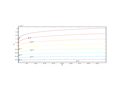
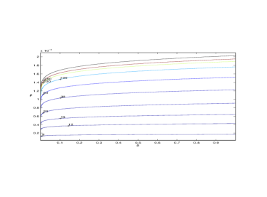
(a)	(b)
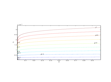
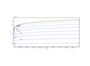
(c)	(d)
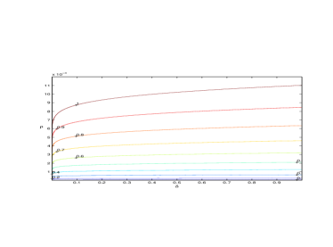
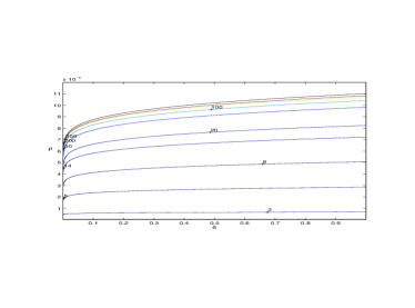
(e)	(f)

Figure 2: For CoSaMP (a-b), SP (c-d), and IHT (e-f) from the left to the right panel: the convergence factor $\mu^{alg}(\delta,\rho)$ and the stability factor $\frac{\xi^{alg}}{1-\mu^{alg}}(\delta,\rho)$.

In the next section, we recall the three algorithms and introduce necessary notation. Then we present the asymmetric restricted isometry property and formulate weaker restricted isometry conditions on a matrix $A$ that ensure the respective algorithm will successfully recover all $k$-sparse signals. In addition to exact recovery, we study the known bounds on the behavior of the algorithms in the presence of noisy measurements. In order to make quantitative comparisons of these results, we must select a matrix ensemble for analysis. In Section 3, we present the lower bounds on the phase transition for each algorithm when the measurement matrix is a Gaussian random matrix. Phase transitions are developed in the case of exact sparse signals while bounds on the multiplicative stability constants are also compared through associated level curves. Section 4 is a discussion of our interpretation of these results and how to use this phase transition framework for comparison of other algorithms.

For an index set $I\subset\{1,\dots,N\}$, let $x_{I}$ denote the restriction of a vector $x\in\mathbb{R}^{N}$ to the set $I$, i.e., $(x_{I})_{i}=x_{i}$ for $i\in I$ and $(x_{I})_{j}=0$ for $j\notin I$. Also, let $A_{I}$ denote the submatrix of $A$ obtained by selecting the columns $A$ indexed by $I$. $A_{I}^{*}$ is the conjugate transpose of $A_{I}$ while $A_{I}^{\dagger}=(A_{I}^{*}A_{I})^{-1}A_{I}^{*}$ is the pseudoinverse of $A_{I}$. In each of the algorithms, thresholding is applied by selecting $m$ entries of a vector with largest magnitude; we refer to this as hard thresholding of magnitude $m$.

2 Greedy Algorithms and the Asymmetric Restricted Isometry Property

2.1 CoSaMP

The CoSaMP recovery algorithm is a support recovery algorithm which applies hard thresholding by selecting the $k$ largest entries of a vector obtained by applying a pseudoinverse to the measurement $y$. In CoSaMP, the columns of $A$ selected for the pseudoinverse are obtained by applying hard thresholding of magnitude $2k$ to $A^{*}$ applied to the residual from the previous iteration and adding these indices to the approximate support set from the previous iteration. This larger pseudoinverse matrix of size $2k\times n$ imposes the most stringent aRIP condition of the three algorithms. However, CoSaMP uses one fewer pseudoinverse per iteration than SP as the residual vector is computed with a direct matrix-vector multiply of size $n\times k$ rather than with an additional pseudoinverse. Furthermore, when computing the output vector $\hat{x}$, CoSaMP does not need to apply another pseudoinverse as does SP. See Algorithm 1.

Algorithm 1 CoSaMP [29]

Input: $A$, $y$, $k$

Output: A $k$-sparse approximation $\hat{x}$ of the target signal $x$

Initialization:

1:  Set $T^{0}=\emptyset$

2:  Set $y^{0}=y$

Iteration: During iteration $l$, do

1:  $\tilde{T}^{l}=T^{l-1}\cup\{2k\ \hbox{indices of largest magnitude entries of}\ A^{*}y^{l-1}\}$

2:  $\tilde{x}=A_{\tilde{T}^{l}}^{\dagger}y$

3:  $T^{l}=\{k\ \hbox{indices of largest magnitude entries of}\ \tilde{x}\}$

4:  $y^{l}=y-A_{T^{l}}\tilde{x}_{T^{l}}$

5:  if $\|y^{l}\|_{2}=0$ then

6:     return  $\hat{x}$ defined by $\hat{x}_{\{1,\dots,N\}-T^{l}}=0$ and $\hat{x}_{T^{l}}=\tilde{x}_{T^{l}}$

7:  else

8:     Perform iteration $l+1$

9:  end if

2.2 Subspace Pursuit

The Subspace Pursuit algorithm is also a support recovery algorithm which applies hard thresholding of magnitude $k$ to a vector obtained by applying a pseudoinverse to the measurements $y$. The submatrix chosen for the pseudoinverse has its columns selected by applying $A^{*}$ to the residual vector from the previous iteration, hard thresholding of magnitude $k$, and adding the indices of the terms to the previous approximate support set. Compared to the other two algorithms, a computational disadvantage of SP is that the aforementioned residual vector is also computed via a pseudoinverse, this time selecting the columns from $A$ by again applying a hard threshold of magnitude $k$. The computation of the approximation to the target signal also requires the application of a pseudoinverse for a matrix of size $n\times k$. See Algorithm 2.

Algorithm 2 Subspace Pursuit [12]

Input: $A$, $y$, $k$

Output: A $k$-sparse approximation $\hat{x}$ of the target signal $x$

Initialization:

1:  Set $T^{0}=\{k\ \hbox{indices of largest magnitude entries of}\ A^{*}y\}$

2:  Set $y_{r}^{0}=y-A_{T^{0}}A_{T^{0}}^{\dagger}y$

Iteration: During iteration $l$, do

1:  $\tilde{T}^{l}=T^{l-1}\cup\{k\ \hbox{indices of largest magnitude entries of}\ A^{*}y_{r}^{l-1}\}$

2:  Set $\tilde{x}=A_{\tilde{T}^{l}}^{\dagger}y$

3:  $T^{l}=\{k\ \hbox{indices of largest magnitude entries of}\ \tilde{x}\}$

4:  $y_{r}^{l}=y-A_{T^{l}}A_{T^{l}}^{\dagger}y$

5:  if $\|y_{r}^{l}\|_{2}=0$ then

6:        return  $\hat{x}$ defined by $\hat{x}_{\{1,\dots,N\}-T^{l}}=0$ and $\hat{x}_{T^{l}}=A_{T^{l}}^{\dagger}y$

7:  else

8:        Perform iteration $l+1$

9:  end if

2.3 Iterative Hard Thresholding

Iterative Hard Thresholding (IHT) is also a support recovery algorithm. However, IHT applies hard thresholding to an approximation of the target signal, rather than to the residuals. This completely eliminates the use of a pseudoinverse, reducing the computational cost per iteration. In particular, hard thresholding of magnitude $k$ is applied to an updated approximation of the target signal, $x$, obtained by matrix-vector multiplies of size $n\times N$ that represent a move by a fixed stepsize $\omega$ along the steepest descent direction from the current iterate for the residual $\|Ax-y\|_{2}^{2}$. See Algorthm 3.

Algorithm 3 Iterative Hard Thresholding [7]

Input: $A$, $y$, $\omega\in(0,1)$, $k$

Output: A $k$-sparse approximation $\hat{x}$ of the target signal $x$

Initialization:

1:  Set $x^{0}=0$

2:  Set $T^{0}=\emptyset$

3:  Set $y^{0}=y$

Iteration: During iteration $l$, do

1:  $x^{l}=x^{l-1}_{T^{l-1}}+wA^{*}y^{l-1}$

2:  $T^{l}=\{k\ \hbox{indices of largest magnitude entries of}\ x^{l}\}$

3:  $y^{l}=y-A_{T^{l}}x_{T^{l}}^{l}$

4:  if $\|y^{l}\|_{2}=0$ then

5:        return  $\hat{x}$ defined by $\hat{x}_{\{1,\dots,N\}-T^{l}}=0$ and $\hat{x}_{T^{l}}=x_{T^{l}}^{l}$

6:  else

7:        Perform iteration $l+1$

8:  end if

Remark 1

(Stopping criteria for greedy methods) In the case of corrupted measurements, where $y=Ax+e$ for some noise vector $e$, the stopping criteria listed in Algorithms 1-3 may never be achieved. Therefore, a suitable alternative stopping criteria must be employed. For our analysis on bounding the error of approximation in the noisy case, we bound the approximation error if the algorithm terminates after $l$ iterations. For example, we could change the algorithm to require a maximum number of iterations $l$ as an input and then terminate the algorithm if our stopping criteria is not met in fewer iterations. In practice, the user would be better served to stop the algorithm when the residual is no longer improving. For a more thorough discussion of suitable stopping criteria for each algorithm in the noisy case, see the original announcement of the algorithms [7, 12, 29].

2.4 The Asymmetric Restricted Isometry Property

In this section we relax the sufficient conditions originally placed on Algorithms 1-3 by employing a more general notion of a restricted isometry. As discussed in [6], the singular values of the $n\times k$ submatrices of an arbitrary measurement matrix $A$ do not, in general, deviate from unity symmetrically. The standard notion of the restricted isometry property (RIP) [10] has an inherent symmetry which is unneccessarily restrictive. Hence, seeking the best possible conditions for the measurement matrix under which Algorithms 1-3 will provably recovery every $k$ sparse vector, we reformulate the sufficient conditions in terms of the asymmetric restricted isometry property (aRIP) [6].

Definition 1

For an $n\times N$ matrix $A$, the asymmetric RIP constants $L(k,n,N)$ and $U(k,n,N)$ are defined as:

$$L(k,n,N) :=\min_{c\geq 0}\,c\,\,\,\mbox{subject to}\,\,\,(1-c)\|x\|_{2}^{2}\leq\|Ax\|_{2}^{2},\,\,\forall x\in\chi^{N}(k);$$ (6)

$$U(k,n,N) :=\min_{c\geq 0}\,c\,\,\,\mbox{subject to}\,\,\,(1+c)\|x\|_{2}^{2}\geq\left\|Ax\right\|_{2}^{2},\,\,\forall x\in\chi^{N}(k).$$ (7)

Remark 2

1. The more common, symmetric definition of the RIP constants is recovered by defining $R(k,n,N)=\max\{L(k,n,N),U(k,n,N)\}$. In this case, a matrix $A$ of size $n\times N$ has the RIP constant $R(k,n,N)$ if

   $$R(k,n,N):=\min_{c\geq 0}\,c\,\,\,\mbox{subject to}\,\,\,(1-c)\|x\|_{2}^{2}\leq\|Ax\|_{2}^{2}\leq(1+c)\|x\|_{2}^{2},\,\,\forall x\in\chi^{N}(k).$$

2. Observe that $\chi^{N}(k)\subset\chi^{N}(k+1)$ for any $k$ and therefore the constants $L(k,n,N)$, $U(k,n,N)$, and $R(k,n,N)$ are nondecreasing in $k$ [10].

3. For all expressions involving $L(\cdot,n,N)$ it is understood, without explicit statement, that the first argument is limited to the range where $L(\cdot,n,N)<1$. Beyond this range of sparsity, there exist vectors which are mapped to zero, and are unrecoverable.

Using the aRIP, we analyze the three algorithms in the case of a general measurement matrix $A$ of size $n\times N$. For each algorithm, the application of Definition 1 results in a relaxation of the conditions imposed on $A$ to provably guarantee recovery of all $x\in\chi^{N}(k)$. We first present a stability result for each algorithm in terms of bounding the approximation error of the output after $l$ iterations. The bounds show a multiplicative stability constant in terms of aRIP contants that amplifies the total energy of the noise. As a corollary, we obtain a sufficient condition on $A$ in terms of the aRIP for exact recovery of all $k$-sparse vectors. The proofs of these results are found in the Appendix. These theorems and corollaries take the same form, differing for each algorithm only by the formulae for various factors. We state the general form of the theorems and corollaries, analogous to Theorem 1 and Corollary 2, and then state the formulae for each of the algorithms CoSaMP, SP, and IHT.

Theorem 3

Given a matrix $A$ of size $n\times N$ with aRIP constants $L(\cdot,n,N)$ and $U(\cdot,n,N)$, for any $x\in\chi^{N}(k)$, let $y=Ax+e$, for some (unknown) noise vector $e$. Then there exists $\mu^{alg}(k,n,N)$ such that if $\mu^{alg}(k,n,N)<1$, the output $\hat{x}$ of algorithm “alg” at the $l^{th}$ iteration approximates $x$ within the bound

$$\|x-\hat{x}\|_{2}\leq\kappa^{alg}(k,n,N)\left[\mu^{alg}(k,n,N)\right]^{l}\|x\|_{2}+\frac{\xi^{alg}(k,n,N)}{1-\mu^{alg}(k,n,N)}\|e\|_{2},$$ (8)

for some $\kappa^{alg}(k,n,N)$ and $\xi^{alg}(k,n,N)$.

Corollary 4

Given a matrix $A$ of size $n\times N$ with aRIP constants $L(\cdot,n,N)$ and $U(\cdot,n,N)$, for any $x\in\chi^{N}(k)$, let $y=Ax$. Then there exists $\mu^{alg}(k,n,N)$ such that if $\mu^{alg}(k,n,N)<1$, the algorithm “alg” exactly recovers $x$ from $y$ and $A$ in a finite number of iterations not to exceed

$$\ell^{alg}_{max}(x):=\left\lceil\frac{\log\nu_{\text{min}}(x)-\log\kappa^{alg}(k,n,N)}{\log\mu^{alg}(k,n,N)}\right\rceil+1$$ (9)

where $\nu_{\text{min}}(x)$ defined as in (5).

We begin with Algorithm 1, the Compressive Sampling Matching Pursuit recovery algorithm of Needell and Tropp [29]. We relax the sufficient recovery condition in [29] via the aRIP.

Theorem 5 (CoSaMP)

Theorem 3 and Corollary 4 are satisfied by CoSaMP, Algorithm 1, with $\kappa^{csp}(k,n,N):=1$ and $\mu^{csp}(k,n,N)$ and $\xi^{csp}(k,n,N)$ defined as

$$\mu^{csp}(k,n,N):=\frac{1}{2}\left(2+\frac{L(4k,n,N)+U(4k,n,N)}{1-L(3k,n,N)}\right)\left(\frac{L(2k,n,N)+U(2k,n,N)+L(4k,n,N)+U(4k,n,N)}{1-L(2k,n,N)}\right)\\$$ (10)

and

$$\xi^{csp}(k,n,N):=2\left\{\left(2+\frac{L(4k,n,N)+U(4k,n,N)}{1-L(3k,n,N)}\right)\left(\frac{\sqrt{1+U(2k,n,N)}}{1-L(2k,n,N)}\right)+\frac{1}{\sqrt{1-L(3k,n,N)}}\right\}.$$ (11)

Next, we apply the aRIP to Algorithm 2, Dai and Milenkovic’s Subspace Pursuit [12]. Again, the aRIP provides a sufficient condition that admits a wider range of measurement matrices than admitted by the symmetric RIP condition derived in [12].

Theorem 6 (SP)

Theorem 3 and Corollary 4 are satisfied by Subspace Pursuit, Algorithm 2, with $\kappa^{sp}(k,n,N)$, $\mu^{sp}(k,n,N)$, and $\xi^{sp}(k,n,N)$ defined as

$$\kappa^{sp}(k,n,N) :=1+\frac{U(2k,n,N)}{1-L(k,n,N)},$$ (12)

$$\mu^{sp}(k,n,N) :=\frac{2U(3k,n,N)}{1-L(k,n,N)}\left(1+\frac{2U(3k,n,N)}{1-L(2k,n,N)}\right)\left(1+\frac{U(2k,n,N)}{1-L(k,n,N)}\right)$$ (13)

and

$$\xi^{sp}(k,n,N) :=\frac{\sqrt{1+U(k,n,N)}}{1-L(k,n,N)}\left[1-\mu^{sp}(k,n,N)+2\kappa^{sp}(k,n,N)\left(1+\frac{2U(3k,n,N)}{1-L(2k,n,N)}\right)\right]$$

$$+\frac{2\kappa^{sp}(k,n,N)}{\sqrt{1-L(2k,n,N)}}.$$ (14)

Finally, we apply the aRIP analysis to Algorithm 3, Iterative Hard Thresholding for Compressed Sensing introduced by Blumensath and Davies [7]. Theorem 7 employs the aRIP to provide a weaker sufficient condition than derived in [7].

Theorem 7 (IHT)

Theorem 3 and Corollary 4 are satisfied by Iterative Hard Thresholding, Algorithm 3, with $\kappa^{iht}(k,n,N):=1$ and $\mu^{iht}(k,n,N)$ and $\xi^{iht}(k,n,N)$ defined as

$$\mu^{iht}(k,n,N):=2\sqrt{2}\max\left\{\omega\left[1+U(3k,n,N)\right]-1,1-\omega\left[1-L(3k,n,N)\right]\right\}.\\$$ (15)

and

$$\xi^{iht}(k,n,N):=2\omega\sqrt{1+U(2k,n,N)}.$$ (16)

Remark 3

Each of Theorems 5, 6 and 7 are derived following the same recipe as in [29], [12] and [7], respectively, using the aRIP rather than the RIP and taking care to maintain the least restrictive bounds at each step (for details, see the Appendix). For Gaussian matrices, the aRIP improves the lower bound on the phase transitions by nearly a multiple of 2 when compared to similar statements using the classical RIP. For IHT, the aRIP is simply a scaling of the matrix so that its RIP bounds are minimal. This is possible for IHT as the factors in $\mu^{iht}(k,n,N)$ involve $L(\alpha k,n,N)$ and $U(\alpha k,n,N)$ for only one value of $\alpha$, here $\alpha=3$. No such scaling interpretation is possible for CoSaMP and SP.

At this point, we digress to mention that the first greedy algorithm shown to have guaranteed exact recovery capability is Needell and Vershynin’s ROMP (Regularized Orthogonal Matching Pursuit) [30]. We omit the algorithm and a rigorous discussion of the result, but state an aRIP condition that will guarantee sparse recovery. ROMP chooses additions to the approximate support sets at each iteration with a regularization step requiring comparability between the added terms. This comparability requires a proof of partitioning a vector of length $N$ into subsets with comparable coordinates, namely the magnitudes of the elements of the subset differ by no more than a factor of 2. The proof that such a partition exists, with each partition having a nonzero energy, forces a pessimistic bound that decays with the problem size.

Theorem 8 (Regularized Orthogonal Matching Pursuit)

Let $A$ be a matrix of size $n\times N$ with aRIP constants $L(2k,n,N)$ and $U(2k,n,N)$. Define

$$\mu^{r}(k,n,N):=U(2k,n,N)\left(1+\frac{1+U(2k,n,N)}{1-L(2k,n,N)}\right).\\$$ (17)

If $\mu^{r}(k,n,N)<\left(1+\sqrt{\frac{5n}{n-1}(\log n+2)}\right)^{-1}$, then ROMP is guaranteed to exactly recover any $x\in\chi^{N}(k)$ from the measurements $y=Ax$ in a finite number of iterations.

Unfortunately, this dependence of the bound on the size of the problem instance forces the result to be inadequate for large problem instances. In fact, this result is inferior to the results for the three algorithms stated above which are all independent of problem size and therefore applicable to the most interesting cases of compressed sensing, when $(k,n,N)\rightarrow\infty$ and $\delta=n/N\rightarrow 0$. It is possible that this dependence on the problem size is an artifact of the technique of proof; without removing this dependence, large problem instances will require the measurement matrix to be a true isometry and the phase transition framework of the next section does not apply.

3 Phase Transitions for Greedy Algorithms with Gaussian Matrices

The quantities $\mu^{alg}(k,n,N)$ and $\xi^{alg}(k,n,N)$ in Theorems 5, 6, and 7 dictate the current theoretical convergence bounds for CoSaMP, SP, and IHT. Although some comparisons can be made between the forms of $\mu^{alg}$ and $\xi^{alg}$ for different algorithms, it is not possible to quantitatively state for what range of $k$ the algorithm will satisfy bounds on $\mu^{alg}(k,n,N)$ and $\xi^{alg}(k,n,N)$ for a specific value of $n$ and $N$. To establish quantitative interpretations of the conditions in Theorems 5, 6 and 7, it is necessary to have quantitative bounds on the behaviour of the aRIP constants $L(k,n,N)$ and $U(k,n,N)$ for the matrix $A$ in question, [4, 6]. Currently, there is no known matrix $A$ for which it has been proven that $U(k,n,N)$ and $L(k,n,N)$ remain bounded above and away from one, respectively, as $n$ grows, for $k$ and $N$ proportional to $n$. However, it is known that for some random matrix ensembles, with exponentially high probability on the draw of $A$, $\frac{1}{1-L(k,n,N)}$ and $U(k,n,N)$ do remain bounded as $n$ grows, for $k$ and $N$ proportional to $n$. The ensemble with the best known bounds on the growth rates of $L(k,n,N)$ and $U(k,n,N)$ in this setting is the Gaussian ensemble. In this section, we consider large problem sizes as $(k,n,N)\rightarrow\infty$, with $\frac{n}{N}\rightarrow\delta$ and $\frac{k}{n}\rightarrow\rho$ for $\delta,\rho\in(0,1)$. We study the implications of the sufficient conditions from Section 2 for matrices with Gaussian i.i.d. entries, namely, entries drawn i.i.d. from the normal distribution with mean $0$ and variance $n^{-1}$, $\mathcal{N}(0,n^{-1})$.

Gaussian random matrices are well studied and much is known about the behavior of their eigenvalues. Edelman [24] derived bounds on the probability distribution functions of the largest and smallest eigenvalues of the Wishart matrices derived from a matrix $A$ with Gaussian i.i.d. entries. Select a subset of columns indexed by $I\subset\{1,\dots,N\}$ with cardinality $k$ and form the submatrix $A_{I}$, and the associated Wishart matrix derived from $A_{I}$ is the matrix $A_{I}^{*}A_{I}$. The distribution of the most extreme eigenvalues of all ${N\choose k}$ Wishart matrices derived from $A$ with Gaussian i.i.d. entries is only of recent interest and the exact probability distribution functions are not known. Recently, using Edelman’s bounds [24], the first three authors [6] derived upper bounds on the probability distribution functions for the most extreme eigenvalues of all ${N\choose k}$ Wishart matrices derived from $A$. These bounds enabled them to formulate upper bounds on the aRIP constants, $L(k,n,N)$ and $U(k,n,N)$, for matrices of size $n\times N$ with Gaussian i.i.d. entries.

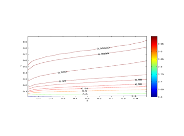
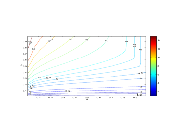
Figure 3: Bounds, $L(\delta,\rho)$ and $U(\delta,\rho)$ (left and right respectively), above which it is exponentially unlikely that the RIP constants $L(k,n,N)$ and $U(k,n,N)$ exceed, with entries in $A$ drawn i.i.d. $N(0,n^{-1})$ and in the limit as $\frac{k}{n}\rightarrow\rho$ and $\frac{n}{N}\rightarrow\delta$ as $n\rightarrow\infty$, see Theorem 9.

Theorem 9 (Blanchard, Cartis, and Tanner [6])

Let $A$ be a matrix of size $n\times N$ whose entries are drawn i.i.d. from ${\cal N}(0,n^{-1})$ and let $n\rightarrow\infty$ with $\frac{k}{n}\rightarrow\rho$ and $\frac{n}{N}\rightarrow\delta$. Let $H(p):=p\log(1/p)+(1-p)\log(1/(1-p))$ denote the usual Shannon Entropy with base $e$ logarithms, and let

$$\psi_{min}(\lambda,\rho) := H(\rho)+\frac{1}{2}\left[(1-\rho)\log\lambda+1-\rho+\rho\log\rho-\lambda\right],$$ (18)

$$\psi_{max}(\lambda,\rho) := \frac{1}{2}\left[(1+\rho)\log\lambda+1+\rho-\rho\log\rho-\lambda\right].$$ (19)

Define $\lambda_{min}(\delta,\rho)$ and $\lambda_{max}(\delta,\rho)$ as the solution to (20) and (21), respectively:

$$\delta\psi_{min}(\lambda_{min}(\delta,\rho),\rho)+H(\rho\delta)=0\quad\mbox{ for }\quad\lambda_{min}(\delta,\rho)\leq 1-\rho$$ (20)

$$\delta\psi_{max}(\lambda_{max}(\delta,\rho),\rho)+H(\rho\delta)=0\quad\mbox{ for }\quad\lambda_{max}(\delta,\rho)\geq 1+\rho.$$ (21)

Define $L(\delta,\rho)$ and $U(\delta,\rho)$ as

$$L(\delta,\rho):=1-\lambda_{min}(\delta,\rho)\quad\hbox{and}\quad U(\delta,\rho):=\min_{\nu\in[\rho,1]}\lambda_{max}(\delta,\nu)-1.$$ (22)

For any $\epsilon>0$, as $n\rightarrow\infty$,

$$\hbox{Prob}\left(L(k,n,N)<L\left(\delta,\rho\right)+\epsilon\right)\rightarrow 1\quad\hbox{and}\quad\hbox{Prob}\left(U(k,n,N)<U\left(\delta,\rho\right)+\epsilon\right)\rightarrow 1.$$

The details of the proof of Theorem 9 are found in [6]. The bounds are derived using a simple union bound over all $N\choose k$ of the $k\times k$ Wishart matrices $A_{I}^{*}A_{I}$ that can be formed from columns of $A$. Bounds on the tail behavior of the probability distribution function for the largest and smallest eigenvalues of $A_{I}^{*}A_{I}$ can be expressed in the form $p(n,\lambda)\exp(n\psi(\lambda,\rho))$ with $\psi$ defined in (18) and (19) and $p(n,\lambda)$ a polynomial. Following standard practices in large deviation analysis, the tails of the probability distribution functionals are balanced against the exponentially large number of Wishart matrices (20) and (21) to define upper and lower bounds on the largest and smallest eigenvalues of all $N\choose k$ Wishart matrices, with bounds $\lambda_{max}(\delta,\rho)$ and $\lambda_{min}(\delta,\rho)$, respectively. Overestimation of the union bound over the combinatorial number of $N\choose k$ Wishart matrices causes the bound $\lambda_{max}(\delta,\rho)$ to not be strictly increasing in $\rho$ for $\delta$ large; to utilize the best available bound on the extreme of the largest eigenvalue, we note that any bound $\lambda_{max}(\delta,\nu)$ for $\nu\in[\rho,1]$ is also a valid bound for submatrices of size $n\times k$. The asymptotic bounds of the aRIP constants, $L(\delta,\rho)$ and $U(\delta,\rho)$, follow directly. See Figure 3 for level curves of the bounds.

With Theorem 9, we are able to formulate quantitative statements about the matrices $A$ with Gaussian i.i.d. entries which satisfy the sufficient aRIP conditions from Section 2. A naive replacement of each $L(\cdot,n,N)$ and $U(\cdot,n,N)$ in Theorems 5-7 with the asymptotic aRIP bounds in Theorem 9 is valid in these cases. The properties necessary for this replacement are detailed in Lemma 16, stated in the Appendix. For each algorithm (CoSaMP, SP and IHT) the recovery conditions can be stated in the same format as Theorem 1 and Corollary 2, with only the expressions for $\kappa(\delta,\rho)$, $\mu(\delta,\rho)$ and $\xi(\delta,\rho)$ differing. These recovery factors are stated in Theorems 10-12.

Theorem 10

Theorem 1 and Corollary 2 are satisfied for CoSaMP, Algorithm 1, with $\kappa^{csp}(\delta,\rho):=1$ and $\mu^{csp}(\delta,\rho)$ and $\xi^{csp}(\delta,\rho)$ defined as

$$\mu^{csp}(\delta,\rho):=\frac{1}{2}\left(2+\frac{L(\delta,4\rho)+U(\delta,4\rho)}{1-L(\delta,3\rho)}\right)\left(\frac{L(\delta,2\rho)+U(\delta,2\rho)+L(\delta,4\rho)+U(\delta,4\rho)}{1-L(\delta,2\rho)}\right).$$ (23)

and

$$\xi^{csp}(\delta,\rho):=2\left\{\left(2+\frac{L(\delta,4\rho)+U(\delta,4\rho)}{1-L(\delta,3\rho))}\right)\left(\frac{\sqrt{1+U(\delta,2\rho)}}{1-L(\delta,2\rho)}\right)+\frac{1}{\sqrt{1-L(\delta,3\rho)}}\right\}.$$ (24)

The phase transition lower bound $\rho_{S}^{csp}(\delta)$ is defined as the solution to $\mu^{csp}(\delta,\rho)=1$. $\rho_{S}^{csp}(\delta)$ is displayed as the black curve in Figure 1(a). $\mu^{csp}(\delta,\rho)$ and $\xi^{csp}(\delta,\rho)/(1-\mu^{csp}(\delta,\rho))$ are displayed in Figure 2 panels (a) and (b) respectively.

Theorem 11

Theorem 1 and Corollary 2 are satisfied for Subspace Pursuit, Algorithm 2, with $\kappa^{sp}(\delta,\rho)$, $\mu^{sp}(\delta,\rho)$, and $\xi^{sp}(\delta,\rho)$ defined as

$$\kappa^{sp}(\delta,\rho) :=1+\frac{U(\delta,2\rho)}{1-L(\delta,\rho)},$$ (25)

$$\mu^{sp}(\delta,\rho) :=\frac{2U(\delta,3\rho)}{1-L(\delta,\rho)}\left(1+\frac{2U(\delta,3\rho)}{1-L(\delta,2\rho)}\right)\left(1+\frac{U(\delta,2\rho)}{1-L(\delta,\rho)}\right),$$ (26)

and

$$\xi^{sp}(\delta,\rho) :=\frac{\sqrt{1+U(\delta,\rho)}}{1-L(\delta,\rho)}\left[1-\mu^{sp}(\delta,\rho)+2\kappa^{sp}(\delta,\rho)\left(1+\frac{2U(\delta,3\rho)}{1-L(\delta,2\rho)}\right)\right]$$

$$+\frac{2\kappa^{sp}(\delta,\rho)}{\sqrt{1-L(\delta,2\rho)}}.$$ (27)

The phase transition lower bound $\rho_{S}^{sp}(\delta)$ is defined as the solution to $\mu^{sp}(\delta,\rho)=1$. $\rho_{S}^{sp}(\delta)$ is displayed as the magenta curve in Figure 1(a). $\mu^{sp}(\delta,\rho)$ and $\xi^{sp}(\delta,\rho)/(1-\mu^{sp}(\delta,\rho))$ are displayed in Figure 2 panels (c) and (d) respectively.

Theorem 12

Theorem 1 and Corollary 2 are satisfied for Iterative Hard Thresholding, Algorithm 3, with $\omega:=2/(2+U(\delta,3\rho)-L(\delta,3\rho))$, $\kappa^{iht}(\delta,\rho):=1$, and $\mu^{iht}(\delta,\rho)$ and $\xi^{iht}(\delta,\rho)$ defined as

$$\mu^{iht}(\delta,\rho):=2\sqrt{2}\left(\frac{L(\delta,3\rho)+U(\delta,3\rho)}{2+U(\delta,3\rho)-L(\delta,3\rho)}\right)$$ (28)

and

$$\xi^{iht}(\delta,\rho):=\frac{4\sqrt{1+U(\delta,2\rho)}}{2+U(\delta,3\rho)-L(\delta,3\rho)}.$$ (29)

The phase transition lower bound $\rho_{S}^{iht}(\delta)$ is defined as the solution to $\mu^{iht}(\delta,\rho)=1$. $\rho_{S}^{iht}(\delta)$ is displayed as the red curve in Figure 1(a). $\mu^{iht}(\delta,\rho)$ and $\xi^{iht}(\delta,\rho)/(1-\mu^{iht}(\delta,\rho))$ are displayed in Figure 2 panels (e) and (f) respectively.

An analysis similar to that presented here for the greedy algorithms CoSaMP, SP, and IHT was previously carried out in [6] for the $\ell_{1}$-regularization problem (2). The form of the results differs from those of Theorem 1 and Corollary 2 in that no algorithm was specified for how (2) is solved. For this reason, no results are stated for the convergence rate or number of iterations. However, (2) can be reformulated as a convex quadratic or second-order cone programming problem — and its noiseless variant as a linear programming — which have polynomial complexity when solved using interior point methods [33]. Moreover, convergence and complexity of other alternative algorithms for solving (2) such as gradient projection have long been studied by the optimization community for more general problems [3, 31, 34], and recently, more specifically for (2) [25, 32] and many more. For completeness, we include the recovery conditions for $\ell_{1}$-regularization derived in [6]; these results follow from the original $\ell_{1}$-regularization bound derived by Foucart and Lai [26] for general $A$.

Theorem 13 (Blanchard, Cartis, and Tanner [6])

Given a matrix $A$ with entries drawn i.i.d. from ${\cal N}(0,n^{-1})$, for any $x\in\chi^{N}(k)$, let $y=Ax+e$ for some (unknown) noise vector $e$. Define

$$\mu^{\ell_{1}}(\delta,\rho):=\frac{1+\sqrt{2}}{4}\left(\frac{1+U(\delta,2\rho)}{1-L(\delta,2\rho)}-1\right)$$ (30)

and

$$\xi^{\ell_{1}}(\delta,\rho):=\frac{3(1+\sqrt{2})}{1-L(\delta,2\rho)}$$ (31)

with $L(\delta,\cdot)$ and $U(\delta,\cdot)$ defined as in Theorem 9. Let $\rho_{S}^{\ell_{1}}(\delta)$ be the unique solution to $\mu^{\ell_{1}}(\delta,\rho)=1$. For any $\epsilon>0$, as $(k,n,N)\rightarrow\infty$ with $n/N\rightarrow\delta\in(0,1)$ and $k/n\rightarrow\rho<(1-\epsilon)\rho_{S}^{\ell_{1}}(\delta)$, there is an exponentially high probability on the draw of $A$ that

$$\hat{x}:=\operatornamewithlimits{arg\,min}_{z}\|z\|_{\ell_{1}}\quad\quad\mbox{ subject to }\quad\|Az-y\|_{2}\leq\|e\|_{2}$$

approximates $x$ within the bound

$$\|x-\hat{x}\|_{2}\leq\frac{\xi^{\ell_{1}}(\delta,(1+\epsilon)\rho)}{1-\mu^{\ell_{1}}(\delta,(1+\epsilon)\rho)}\|e\|_{2}.$$ (32)

$\rho_{S}^{\ell_{1}}(\delta)$ is displayed as the blue curve in Figure 1(a). $\mu^{\ell_{1}}(\delta,\rho)$ and $\xi^{\ell_{1}}(\delta,\rho)/(1-\mu^{\ell_{1}}(\delta,\rho))$ are displayed in Figure 4 panels (c) and (d) respectively.

Corollary 14 (Blanchard, Cartis, and Tanner [6])

Given a matrix $A$ with entries drawn i.i.d. from ${\cal N}(0,n^{-1})$, for any $x\in\chi^{N}(k)$, let $y=Ax$. For any $\epsilon>0$, with $n/N\rightarrow\delta\in(0,1)$ and $k/n\rightarrow\rho<(1-\epsilon)\rho_{S}^{\ell_{1}}(\delta)$ as $(k,n,N)\rightarrow\infty$, there is an exponentially high probability on the draw of $A$ that

$$\hat{x}:=\operatornamewithlimits{arg\,min}_{z}\|z\|_{\ell_{1}}\quad\quad\mbox{ subject to }\quad Az=y$$

exactly recovers $x$ from $y$ and $A$.

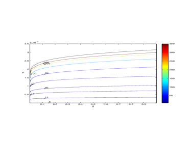
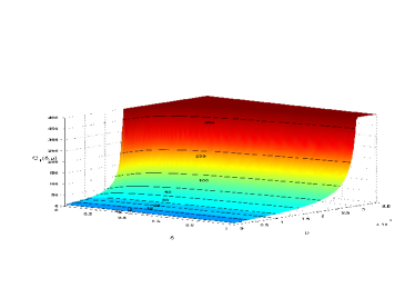
(a)	(b)

Figure 4: (a): level curves for specific values of $\frac{\xi}{1-\mu}(\delta,\rho)$ for $\ell_{1}$-regularization respectively. (b): the surface whose level curves specify the multiplicative stability constants for $\ell_{1}$-regularization.

4 Discussion and Conclusions

Summary

We have presented a framework in which recoverability results for sparse approximation algorithms derived using the ubiquitous RIP can be easily compared. This phase transition framework, [16, 20, 21, 6], translates the generic RIP-based conditions of Theorem 3 into specific sparsity levels $k$ and problem sizes $n$ and $N$ for which the algorithm is guaranteed to satisfy the sufficient RIP conditions with high probability on the draw of the measurement matrix; see Theorem 1. Deriving (bounds on) the phase transitions requires bounds on the behaviour of the measurement matrix’ RIP constants [4]. To achieve the most favorable quantitative bounds on the phase transitions, we used the less restrictive aRIP constants; moreover, we employed the best known bounds on aRIP constants, those provided for Gaussian matrices [6], see Theorem 9.

This framework was illustrated on three exemplar greedy algorithms: CoSaMP [29], SP [12], and IHT [7]. The lower bounds on the phase transitions in Theorems 10-12 allow for a direct comparison of the current theoretical results/guarantees for these algorithms.

Computational Cost of CoSaMP, SP and IHT

The major computational cost per iteration in these algorithms is the application of one or more pseudoinverses. SP uses two pseudoinverses of dimensions $k\times n$ per iteration and another to compute the output vector $\hat{x}$; see Algorithm 2. CoSaMP uses only one pseudoinverse per iteration but of dimensions $2k\times n$; see Algorithm 1. Consequently, CoSaMP and SP have identical computational cost per iteration, of order $kn^{2}$, if the pseudoinverse is solved using an exact $QR$ factorization. IHT avoids computing a pseudoinverse altogether in internal iterations, but is aided by one pseudoinverse of dimensions $k\times n$ on the final support set. Thus IHT has a substantially lower computational cost per iteration than CoSaMP and SP. Note that pseudoinverses may be computed approximately by an iterative method such as conjugate gradients [29]. As such, the exact application of a pseudoinverse could be entirely avoided, improving the implementation costs of these algorithms, especially of CoSaMP and SP.

Globally, all three algorithms converge linearly; in fact, they converge in a finite number of iterations provided there exists a $k$-sparse solution to $Ax=y$ and a sufficient aRIP condition is satisfied, see Corollary 2. For each algorithm, the upper bound on the required number of iterations grows unbounded as the function $\mu^{alg}(k,n,N)\rightarrow 1$. Hence, according to the bounds presented here, to ensure rapid convergence, it is advantageous to have a matrix that satisfies a more strict condition, such as $\mu^{alg}(k,n,N)<\frac{1}{2}$. Similarly, the factor controlling stability to additive noise, namely the vector $e$ in Theorem 1, blows up as the function $\mu^{alg}(k,n,N)\rightarrow 1$. Again, according to the bounds presented here, in order to guarantee stability with small amplification of the additive noise, it is necessary to restrict the range of $\frac{\xi^{alg}}{1-\mu^{alg}}(k,n,N)$. A phase transition function analogous to the functions $\rho_{S}^{alg}(\delta)$ can be easily computed in these settings as well, resulting in curves lower than those presented in Figure 1(a). This is the standard trade-off of compressed sensing, where one must determine the appropriate balance between computational efficiency, stability, and minimizing the number of measurements.

Comparison of Phase Transitions and Constants of Proportionality

From Figure 1(a), we see that the best known lower bounds on the phase transitions for the three greedy algorithms satisfy the ordering $\rho_{S}^{csp}(\delta)<\rho_{S}^{sp}(\delta)<\rho_{S}^{iht}(\delta)$ for Gaussian measurement matrices. Therefore, we now know that, at least for Gaussian matrices, according to existing thoery, IHT has the largest region where recovery for all signals can be guaranteed; the regions with similar guarantees for SP and CoSaMP are considerably smaller. Moreover, IHT has a lower bound on its computational cost.

The phase transition bounds $\rho_{S}^{alg}(\delta)$ also allow a precise comparison of the recoverability results derived for these greedy algorithms with those proven for $\ell_{1}$-regularization using the aRIP, see Figure 1. Although [29, 12, 7] have provided guarantees of successful sparse recovery analogous to those for $\ell_{1}$-regularization, the greedy algorithms place a more restrictive aRIP condition on the suitable matrices to be used in the algorithm. However, some of the algorithms for solving the $\ell_{1}$-regularization problem, such as interior point methods, are, in general, computationally more expensive that the greedy methods discussed in this paper, and hence attention needs to be paid to the method of choice for solving the $\ell_{1}$-regularization problem [2, 25].

The lower bounds on the phase transitions presented here can also be read as lower bounds on the constant of proportionality in the oversampling rate, namely, taking $n\geq(\rho^{alg}_{S}(\delta))^{-1}k$ measurements rather than the oracle rate of $k$ measurements is sufficient if algorithm “alg” is used to recover the $k$-sparse signal. From Figure 1(b), it is clear that according to the conditions presented here, the convergence of greedy algorithms can only be guaranteed with substantially more measurements than for $\ell_{1}$-regularization. The lowest possible number of measurements (when $n=N$ so $\delta=1$) for the algorithms are as follows: $n\geq 907k$ for IHT, $n\geq 3124k$ for SP, and $n\geq 4923k$ for CoSaMP. On the other hand, an aRIP analysis of $\ell_{1}$-regularization yields that linear programming requires $n\geq 317k$. In fact, using a geometric, convex polytopes approach, Donoho has shown that for $\ell_{1}$-regularization, $n\geq 5.9k$ is a sufficient number of measurements [6, 16, 18] when the target signal, $x$, is exactly $k$-sparse, and the multiple 5.9 increases smoothly as noise is added [38].

Future Improvements and Conclusions

The above bounds on greedy algorithms’ phase transitions could be improved by further refining the algorithms’ theory, namely, deriving less strict aRIP conditions on the measurement matrix that still ensure convergence of the algorithm; as the latter is an active research topic, we expect such developments to take place. The phase transition framework presented here may also be applied to such advances. Alternatively, increasing the lower bounds on the phase transitions could be expected to occur from improving the upper bounds we employed on the aRIP constants of the Gaussian measurement matrices, see Theorem 9. However, extensive empirical calculations of lower estimates of aRIP constants show the latter to be within a factor of $1.83$ of our proven upper bounds [6]. During the revision of this manuscript, improved bounds on the aRIP constants for the Gaussian ensemble were derived [1], tightening the bound to be within $1.57$ of lower estimates. However, for $\rho\approx 10^{-3}$ both bounds were already very sharp [1], and the resulting increase of the phase transitions shown here was under 0.5%.

Appendix A Proofs of Main Results

We present a framework by which RIP-based convergence results of the form presented in Theorem 3 can be translated into results of the form of Theorem 1; that is removing explicit dependencies on RIP constants in favour of their bounds.

The proofs of Theorems 5, 6, and 7 rely heavily on a sequence of properties of the aRIP constants, which are summarize in Lemma 15 and proven in Section A.1. Theorems 10, 11, and 12 follow from Theorems 5, 6, and 7 and the form of $\mu^{alg}$ and $\xi^{alg}$ as functions of $L$ and $U$; this latter point is summarized in Lemma 16 which is stated and proven in Section A.1. The resulting Theorems 10, 11, and 12 can then be interpreted in the phase transition framework advocated by Donoho et al. [16, 18, 19, 20, 22], as we have explained in Section 4.

The remainder of the Appendix is organized by algorithms, with each subsection first proving convergence bounds for generic aRIP bounds, followed by the Gaussian specific variants as functions of $(\delta,\rho)$. For the results pertaining to $\ell_{1}$-regularization, the reader is directed to [6].

A.1 Technical Lemmas

Throughout the analysis of the algorithms, we repeatedly use implications of the aRIP on a matrix $A$ as outlined in Lemma 15. This lemma has been proven in the symmetric case repeatedly in the literature; we include the proof of the asymmetric variant for completeness.

Recall that for some index sets $I,J\subset\{1,\dots,N\}$, the restriction of a vector $x$ to the set $I$ is denoted $x_{I}$; i.e. $(x_{I})_{i}=x_{i}$ for $i\in I$ and $(x_{I})_{i}=0$ for $i\notin I$. Furthermore, the submatrix of $A$ derived by selecting the columns of $A$ indexed by $I$ is denoted $A_{I}$. In either case, $x_{I-J}$ denoted the restriction of $x$ to the set of indices in $I$ that are not in $J$; likewise $A_{I-J}$ is the submatrix formed by columms of $A$ indexed by the set $I-J$. Finally, let $\mathbb{R}^{I}$ denote the set of vectors in $\mathbb{R}^{N}$ whose support is contained in $I$.

Lemma 15 (Implications of aRIP)

Let $I$ and $J$ be two disjoint index sets, namely $I,J\subset\left\{1,\dots,N\right\}$; $I\cap J=\emptyset$. Suppose $A$ is a matrix of size $n\times N$ with aRIP constants $L(|I|+|J|,n,N)$ and $U(|I|+|J|,n,N)$, and let $u\in\mathbb{R}^{I}$, $v\in\mathbb{R}^{J}$, $y\in\mathbb{R}^{n}$, $\omega\in(0,1)$, and $Id$ the identity matrix of appropriate size. Then Definition 1 implies each of the following:

1. $\left\|A_{I}^{*}y\right\|_{2}\leq\sqrt{1+U(|I|,n,N)}\|y\|_{2}$

2. $(1-L(|I|,n,N))\|u\|_{2}\leq\left\|A_{I}^{*}A_{I}u\right\|_{2}\leq(1+U(|I|,n,N))\|u\|_{2}$

3. $\left\|A_{I}^{\dagger}y\right\|_{2}\leq(1-L(|I|,n,N))^{-\frac{1}{2}}\|y\|_{2}$

4. $\left|\left\langle A_{I}u,A_{J}v\right\rangle\right|\leq\frac{1}{2}\left(L(|I|+|J|,n,N)+U(|I|+|J|,n,N)\right)\|u\|_{2}\|v\|_{2}$

5. $\left\|A_{I}^{*}A_{J}v\right\|_{2}\leq U(|I|+|J|,n,N)\|v\|_{2}$.

6. $\left\|(Id-\omega A_{I}^{*}A_{I})u\right\|_{2}\leq\max\left\{\omega(1+U(|I|,n,N))-1,1-\omega(1-L(|I|,n,N))\right\}\|u\|_{2}.$

Proof 1

From Remark 2, it is clear that the aRIP constants are nondecreasing in the first argument pertaining the sparsity level. Therefore, $A$ must also have the aRIP constants $L(|I|,n,N)\leq L(|I|+|J|,n,N)$ and $U(|I|,n,N)\leq U(|I|+|J|,n,N)$. Also, Definition 1 implies that the singular values of the submatrix $A_{I}$ are contained in the interval $[\sqrt{1-L(|I|,n,N)},\sqrt{1+U(|I|,n,N)}]$. Thus, (i)-(iii) follow from the standard relationships between the singular values of $A_{I}$ and the associated matrix in (i)-(iii).

To prove (iv), let $m=|I|+|J|$. We may assume $\left\|u\right\|_{2}=\|v\|_{2}=1$; otherwise we normalize the vectors. Let $\alpha=A_{I}u$ and $\beta=A_{J}v$. Then, since $I\cap J=\emptyset$,

$$\left\|\alpha\pm\beta\right\|_{2}^{2}=\left\|A_{I}u\pm A_{J}v\right\| =\left\|\left[A_{I},A_{J}\right]\left[\begin{array}[]{c}u\\ \pm v\end{array}\right]\right\|_{2}$$ (35)

$$\left\|\left[\begin{array}[]{c}u\\ \pm v\end{array}\right]\right\|_{2}^{2}=\left\|u\right\|_{2}^{2}+\left\|v\right\|_{2}^{2} =2.$$ (38)

$\left[A_{I},A_{J}\right]$ is a submatrix of $A$ of size $n\times m$, so applying Definition 1 to the right most portion of (35) and invoking (38), we have

$$2\left(1-L(m,n,N)\right)\leq\|\alpha\pm\beta\|_{2}^{2}\leq 2\left(1+U(m,n,N)\right).$$ (39)

By polarization and (39),

$$\left\langle\alpha,\beta\right\rangle=\frac{\left\|\alpha+\beta\right\|_{2}^{2}-\left\|\alpha-\beta\right\|_{2}^{2}}{4} \leq\frac{L(m,n,N)+U(m,n,N)}{2}$$

$$\hbox{and}\qquad-\left\langle\alpha,\beta\right\rangle=\frac{\left\|\alpha-\beta\right\|_{2}^{2}-\left\|\alpha+\beta\right\|_{2}^{2}}{4} \leq\frac{L(m,n,N)+U(m,n,N)}{2}.$$

Thus $|\left\langle A_{I}u,A_{J}v\right\rangle|=|\left\langle\alpha,\beta\right\rangle|\leq\left(L(m,n,N)+U(m,n,N)\right)/2$, establishing (iv).

Since $I\cap J=\emptyset$, the matrix $-A_{I}^{*}A_{J}$ is a submatrix of $Id_{I\cup J}-A_{I}^{*}A_{J}$. To establish (v), we observe that the aRIP implies that the eigenvalues of every size $n\times m$ submatrix of $A$ lie in the interval $[1-L(m,n,N),1+U(m,n,N)]$. Thus the eigenvalues of $Id_{I\cup J}-A_{I}^{*}A_{J}$ must lie in $[0,U(m,n,N)]$. Therefore $\left\|A_{I}^{*}A_{J}v\right\|_{2}^{2}=\left\|-A_{I}^{*}A_{J}v\right\|_{2}^{2}$ completes the proof of (v).

To prove (vi), note that $\|(Id-\omega A_{I}^{*}A_{I})\|_{2}$ is bounded above by the maximum magnitude of the eigenvalues of $(\omega A_{I}^{*}A_{I}-Id)$, which lie in the interval with endpoints $\omega(1-L(|I|,n,N))-1$ and $\omega(1+U(|I|,n,N))-1$.

Theorems 10, 11, and 12 follow from Theorems 5, 6, and 7 and the form of $\mu^{alg}$ and $\xi^{alg}$ as functions of $L$ and $U$. We formalize the relevant functional dependencies in the next three lemmas.

Lemma 16

For some $\tau<1$, define the set $\mathcal{Z}:=(0,\tau)^{p}\times(0,\infty)^{q}$ and let $F:\mathcal{Z}\rightarrow\mathbb{R}$ be continuously differentiable on $\mathcal{Z}$. Let $A$ be a Gaussian matrix of size $n\times N$ with aRIP constants $L(\cdot,n,N),U(\cdot,n,N)$ and let $L(\delta,\cdot),U(\delta,\cdot)$ be defined as in Theorem 9. Define $1$ to be the vector of all ones, and

$$z(k,n,N) :=[L(k,n,N),\dots,L(pk,n,N),U(k,n,N),\dots,U(qk,n,N)]$$ (40)

$$z(\delta,\rho) :=[L(\delta,\rho),\dots,L(\delta,p\rho),U(\delta,\rho),\dots,U(\delta,q\rho)].$$ (41)

1. Suppose, for all $t\in\mathcal{Z}$, $\left(\nabla F[t]\right)_{i}\geq 0$ for all $i=1,\dots,p+q$ and for any $v\in\mathcal{Z}$ we have $\nabla F[t]\cdot v>0$. Then for any $c\epsilon>0$, as $(k,n,N)\rightarrow\infty$ with $\frac{n}{N}\rightarrow\delta,\frac{k}{n}\rightarrow\rho$, there is an exponentially high probability on the draw of the matrix $A$ that

   $$\hbox{Prob}\left(F[z(k,n,N)]<F[z(\delta,\rho)+1c\epsilon]\right)\rightarrow 1\qquad\hbox{as}\ n\rightarrow\infty.$$ (42)

2. Suppose, for all $t\in\mathcal{Z}$, $\left(\nabla F[t]\right)_{i}\geq 0$ for all $i=1,\dots,p+q$ and there exists $j\in\{1,\dots,p\}$ such that $\left(\nabla F[t]\right)_{j}>0$. Then there exists $c\in(0,1)$ depending only on $F,\delta$,and $\rho$ such that for any $\epsilon\in(0,1)$

   $$F[z(\delta,\rho)+1c\epsilon]<F[z(\delta,(1+\epsilon)\rho)],$$ (43)

   and so there is an exponentially high probability on the draw of $A$ that

   $$\hbox{Prob}\left(F[z(k,n,N)]<F[z(\delta,(1+\epsilon)\rho)]\right)\rightarrow 1\qquad\hbox{as}\ n\rightarrow\infty.$$ (44)

   Also, $F(z(\delta,\rho))$ is strictly increasing in $\rho$.

Proof 2

To prove (i), suppose $u,v\in\mathcal{Z}$ with $v_{i}>u_{i}$ for all $i=1,\dots,p+q$. From Taylor’s Theorem, $F[v]=F[u+(v-u)]=F[u]+\nabla F[t]\cdot[v-u]$ with $t=u+\lambda[v-u]$ for some $\lambda\in(0,1)$. Then

$$F[v]>F[u]$$ (45)

since, by assumption, $\nabla F[t]\cdot[v-u]>0$.

From Theorem 9, for any $c\epsilon>0$ and any $i=1,\dots,p+q$, as $(k,n,N)\rightarrow\infty$ with $\frac{n}{N}\rightarrow\delta$, $\frac{k}{n}\rightarrow\rho$,

$$\hbox{Prob}\left(z(k,n,N)_{i}<z(\delta,\rho)_{i}+c\epsilon\right)\rightarrow 1,$$

with convergence to $1$ exponential in $n$. Therefore, letting $v_{i}:=z(\delta,\rho)_{i}+c\epsilon$ and $u_{i}:=z(k,n,N)_{i}$, for all $i=1,\dots,p+q$, we conclude from (45) that

$$\hbox{Prob}(F[z(k,n,N)]<F[z(\delta,\rho)+1c\epsilon])\rightarrow 1,$$

again with convergence to $1$ exponential in $n$.

To establish (ii), we take the Taylor expansion of $F$ centered at $z(\delta,\rho)$, namely

$$F[z(\delta,\rho)+1c\epsilon] =F[z(\delta,\rho)]+\nabla F[t_{1}]\cdot 1c\epsilon\quad\hbox{for}\ t_{1}\in(z(\delta,\rho),z(\delta,\rho)+1c\epsilon)$$ (46)

$$F[z(\delta,(1+\epsilon)\rho)] =F[z(\delta,\rho)]+\left.\left(\nabla F[z(\delta,\rho)]\cdot\frac{\partial}{\partial\rho}z(\delta,\rho)\right)\right|_{\rho=t_{2}}\epsilon\rho\quad\hbox{for}\ t_{2}\in(\rho,(1+\epsilon)\rho).$$ (47)

Select

$$t_{1}^{\star} =\hbox{argmax}\left\{\nabla F[t_{1}]:t_{1}\in[z(\delta,\rho),z(\delta,\rho)+1]\right\}$$

$$t_{2}^{\star} =\hbox{argmin}\left\{\left.\left(\nabla F[z(\delta,\rho)]\cdot\frac{\partial}{\partial\rho}z(\delta,\rho)\right)\right|_{\rho=t_{2}}:t_{2}\in[\rho,(1+\epsilon)\rho]\right\}$$

so that

$$F[z(\delta,\rho)+1c\epsilon] \leq F[z(\delta,\rho)]+\nabla F[t_{1}^{\star}]\cdot 1c\epsilon$$ (48)

$$F[z(\delta,(1+\epsilon)\rho)] \geq F[z(\delta,\rho)]+\left.\left(\nabla F[z(\delta,\rho)]\cdot\frac{\partial}{\partial\rho}z(\delta,\rho)\right)\right|_{\rho=t_{2}^{\star}}\epsilon\rho.$$ (49)

Since $L(\delta,\rho)$ is strictly increasing in $\rho$ [6], then $\left(\left.\frac{\partial}{\partial\rho}z(\delta,\rho)\right|_{\rho=t_{2}^{\star}}\right)_{j}>0$ for all $j=1,\dots,p$. Since $U(\delta,\rho)$ is nondecreasing in $\rho$ [6], then $\left(\left.\frac{\partial}{\partial\rho}z(\delta,\rho)\right|_{\rho=t_{2}^{\star}}\right)_{i}\geq 0$ for all $i=p+1,\dots,p+q$. Hence, by the hypotheses of (ii),

$$\left.\left(\nabla F[z(\delta,\rho)]\cdot\frac{\partial}{\partial\rho}z(\delta,\rho)\right)\right|_{\rho=t_{2}^{\star}} >0$$

$$\nabla F[t_{1}^{\star}]\cdot 1 >0.$$

Therefore, for any $c$ satisfying

$$0<c<\min\left\{1,\rho\frac{\left.\left(\nabla F[z(\delta,\rho)]\cdot\frac{\partial}{\partial\rho}z(\delta,\rho)\right)\right|_{\rho=t_{2}^{\star}}}{\nabla F[t_{1}^{\star}]\cdot 1}\right\},$$

(48) and (49) imply (43). Since the hypotheses of (ii) imply those of (i), (42) also holds, and so (44) follows. $F(z(\delta,\rho))$ strictly increasing follows from the hypotheses of (ii) and $L(\delta,\rho)$ and $U(\delta,\rho)$ strictly increasing and nondecreasing in $\rho$, respectively [6].

Let the superscript $alg$ denote the algorithm identifier so that $\mu^{alg}(k,n,N)$ is defined by one of (10), (13), (15), while $\mu^{alg}(\delta,\rho)$ is defined by one of (23), (26), (28). Next, a simple property is summarized in Lemma 17, that further reveals some necessary ingredients of our analysis.

Lemma 17

Assume that $\mu^{alg}(\delta,\rho)$ is strictly increasing in $\rho$ and let $\rho_{S}^{alg}(\delta)$ solve $\mu^{alg}(\delta,\rho)=1$. For any $\epsilon\in(0,1)$, if $\rho<(1-\epsilon)\rho_{S}^{alg}(\delta)$, then $\mu^{alg}(\delta,(1+\epsilon)\rho)<1$.

Proof 3

Let $\rho^{alg}_{\epsilon}(\delta)$ be the solution to $\mu^{alg}(\delta,(1+\epsilon)\rho)=1$. Since by definition, $\rho_{S}^{alg}(\delta)$ denotes a solution to $\mu^{alg}(\delta,\rho)=1$, and this solution is unique as $\mu^{alg}(\delta,\rho)$ is strictly increasing, we must have $(1+\epsilon)\rho^{alg}_{\epsilon}(\delta)=\rho_{S}^{alg}(\delta)$. Since $(1-\epsilon)<(1+\epsilon)^{-1}$ for all $\epsilon\in(0,1)$, we have $(1-\epsilon)\rho_{S}^{alg}(\delta)<\rho_{\epsilon}^{alg}(\delta)$. If $\rho<(1-\epsilon)\rho_{S}^{alg}(\delta)$, then since $\mu^{alg}(\delta,\rho)$ is strictly increasing in $\rho$,

$$\mu^{alg}(\delta,(1+\epsilon)\rho)<\mu^{alg}(\delta,(1+\epsilon)(1-\epsilon)\rho_{S}^{alg}(\delta))<\mu^{alg}(\delta,(1+\epsilon)\rho_{\epsilon}^{alg}(\delta))=1.$$

Note that Lemma 16 ii) with $F:=\mu^{alg}$ will be employed to show the first assumption in Lemma 17; this is but one of several good uses of Lemma 16 that we will make.

Corollaries 2 and 4 are easily derived from Lemma 18. Note that this lemma demonstrates only that the support set has been recovered. The proof of Lemma 18 is a minor generalization of a proof from [12, Theorem 7].

Lemma 18

Suppose, after $l$ iterations, algorithm $alg$ returns the $k$-sparse approximation $\hat{x}^{l}$ to a $k$-sparse target signal $x$. Suppose there exist constants $\mu$ and $\kappa$ independent of $l$ and $x$ such that

$$\|x-\hat{x}^{l}\|_{2}\leq\kappa\mu^{l}\|x\|_{2}.$$ (50)

If $\mu<1$, then the support set of $\hat{x}^{l}$ coincides with the support set of $x$ after at most $\ell_{max}^{alg}(x)$ iterations, where

$$\ell_{max}^{alg}(x):=\left\lceil\frac{\log\frac{1}{\kappa}\nu_{min}(x)}{\log\mu}\right\rceil+1,$$ (51)

where $\nu_{\text{min}}(x)$ is defined in (5).

Proof 4

Let $T$ be the support set of $x$ and $T^{l}$ be the support set of $\hat{x}^{l}$; as $x,\hat{x}^{l}\in\chi^{N}(k)$, $|T|,|T^{l}|\leq k$. From the definition (51) of $\ell_{max}^{alg}(x)$ and (5), $\kappa\mu^{\ell_{max}^{alg}(x)}\|x\|_{2}<\min_{i\in T}|x_{i}|$. From (50), we then have

$$\|x-\hat{x}^{\ell_{max}^{alg}(x)}\|_{2}\leq\kappa\mu^{\ell_{max}^{alg}(x)}\|x\|_{2}<\min_{i\in T}|x_{i}|$$

which clearly implies that $T\subset T^{\ell_{max}^{alg}(x)}$. Since $|T|=|T^{\ell_{max}^{alg}(x)}|$, the sets must be equal.

Theorems 5, 6 and 7 define the constants $\mu=\mu^{alg}(k,n,N)$ and $\kappa$ to be used in Lemma 18 for proving Corollary 4. For CoSaMP and IHT, $\kappa=\kappa^{alg}(k,n,N)=1$. For SP, the term involving $\kappa$ is removed by combining Lemmas 23 and 24 (with $e=0$) to obtain

$$\|x_{T-T^{l}}\|_{2}\leq\mu^{sp}(k,n,N)\|x_{T-T^{l-1}}\|_{2};$$ (52)

applying (52) iteratively provides

$$\|x_{T-T^{l}}\|_{2}\leq\mu^{sp}(k,n,N)^{l}\|x\|_{2}.$$ (53)

which again, gives $\kappa=1$. Similarly, Theorems 10, 11 and 12 define the constants $\mu=\mu^{alg}(\delta,\rho)$ and $\kappa$ to be used in Lemma 18 for proving Corollary 2, with the above comments on the IHT choice of $\kappa$ also applying in this case.

To ensure exact recovery of the target signal, namely, to complete the proof of Corollaries 2 and 4, we actually need something stronger than recovering the support set as implied by Lemma 18. For CoSaMP and SP, since the algorithms employ a pseudoinverse at an appropriate step, the output is then the exact sparse signal. For IHT, no pseudoinverse has been applied; thus, to recover the signal exactly, one simply determines $T$ from the output vector and then $x=A_{T}^{\dagger}y$. These comments and Lemma 18 now establish Corollaries 2 and 4 for each algorithm, and we will not restate the proof for each individual algorithm.

In each of the following subsections, we first consider the case of general measurement matrices, $A$, and prove the results from Section 2 which establish an aRIP condition for an algorithm. We then proceed to choose a specific matrix ensemble, matrices with Gaussian i.i.d. entries, for which Section 3 establishes lower bounds on the phase transition for exact recovery of all $x\in\chi^{N}(k)$ and then provide probabilistic bounds on the multiplicative stability factors.

A.2 Proofs for CoSaMP

In this section we prove the results from Sections 2 and 3 reported for CoSaMP [29]. The proofs mimic those of Needell and Tropp while employing the aRIP constants. In each proof, the smallest possible support is retained for the aRIP constants in order to acquire from this method of analysis the best possible conditions on the measurement matrix used in the CoSaMP algorithm. This change is in many cases straightforward, requiring only a substitution of $U(ak,n,N)$ or $L(ak,n,N)$ for $R(ak,n,N)$, for some $a\in\{2,3,4\}$. In such cases we simply restate the result. Where there is a more substantial change, we provide fuller details of the proof.

The argument proceeds in [29] by establishing bounds on the approximation error at a given iteration in terms of the approximation error at the previous iteration, and the energy of the noise. Since each iteration of the CoSaMP algorithm consists of essentially four steps, this was achieved by a series of four lemmas [29, Lemmas 4.2 to 4.5], one for each step. We restate [29, Lemmas 4.3 and 4.5] (the support merger and pruning steps respectively) without any alteration, and provide an outline of how the proofs of [29, Lemmas 4.2 and 4.4] (identification and estimation) can be adapted. To simplify the working, we follow [29] and introduce some further notation: let the set of $2k$ indices corresponding to the largest magnitude entries of $A^{\ast}y^{l-1}$ in Step 1 of Algorithm 1 be denoted by $\Omega$. Also let $r=\tilde{x}_{T^{l-1}}-x$ be the error in the approximation from the previous iteration, and let $R$ be the support set of $r$, so that $|R|\leq 2k$.

Lemma 19

After the identification step, we have

$$\|r_{\Omega^{C}}\|_{2}\leq\left(\frac{L(2k,n,N)+U(2k,n,N)+L(4k,n,N)+U(4k,n,N)}{2(1-L(2k,n,N))}\right)\|r\|_{2}+2\frac{\sqrt{1+U(2k,n,N)}}{1-L(2k,n,N)}\|e\|_{2}.$$

Proof 5

By Lemma 15, we have

$$\|y^{l}_{(\Omega-R)}\|_{2}\leq\frac{1}{2}(L(4k,n,N)+U(4k,n,N))\|r\|_{2}+\sqrt{1+U(2k,n,N)}\|e\|_{2},\;\;\;\mbox{and}$$

$$\|y^{l}_{(R-\Omega)}\|_{2}\geq(1-L(2k,n,N))\|r_{(R-\Omega)}\|_{2}-\frac{1}{2}(L(2k,n,N)+U(2k,n,N))\|r\|_{2}-\sqrt{1+U(2k,n,N)}\|e\|_{2}.$$

The result now follows by rearrangement.

Lemma 20

After the support merger step, we have

$$\|x_{(\tilde{T}^{l})^{C}}\|_{2}\leq\|r_{\Omega^{C}}\|_{2}.$$

Lemma 21

After the estimation step, we have

$$\|x-\tilde{x}\|_{2}\leq\left(1+\frac{L(4k,n,N)+U(4k,n,N)}{2(1-L(3k,n,N))}\right)\|x_{(\tilde{T}^{l})^{C}}\|_{2}+\frac{1}{\sqrt{1-L(3k,n,N)}}\|e\|_{2}.$$

Proof 6

Using Lemma 15, we have

$$\|x_{\tilde{T}^{l}}-\tilde{x}_{\tilde{T}^{l}}\|_{2}\leq\frac{L(4k,n,N)+U(4k,n,N)}{2(1-L(3k,n,N))}\|x_{(\tilde{T}^{l})^{C}}\|_{2}+\frac{1}{\sqrt{1-L(3k,n,N)}}\|e\|_{2},$$

which combines with $\|x-\tilde{x}\|_{2}\leq\|x_{(\tilde{T}^{l})^{C}}\|_{2}+\|x_{\tilde{T}^{l}}-\tilde{x}_{\tilde{T}^{l}}\|_{2}$ to give the required result.

Lemma 22

After the pruning step, we have

$$\|x-\tilde{x}_{T^{l}}\|_{2}\leq 2\|x-\tilde{x}\|_{2}.$$

The preceding lemmas facilitate the proof of Theorem 5.

Proof 7 (Theorem 5)

By Lemmas 21 and 22, we have

$$\begin{array}[]{rcl}\|x-\tilde{x}_{T^{l}}\|_{2}&\leq&2\|x-\tilde{x}\|_{2}\\ &\leq&\left(2+\frac{L(4k,n,N)+U(4k,n,N)}{1-L(3k,n,N)}\right)\|x_{(\tilde{T}^{l})^{C}}\|_{2}+\frac{2}{\sqrt{1-L(3k,n,N)}}\|e\|_{2}.\end{array}$$

Now by Lemma 20, $\|x_{(\tilde{T}^{l})^{C}}\|_{2}$ is bounded above by $\|r_{\Omega^{C}}\|_{2}$. Then applying Lemma 19 and simplifying, we obtain

$$\|\tilde{x}_{T^{l}}-x\|_{2}\leq\mu^{csp}(k,n,N)\|\tilde{x}_{T^{l-1}}-x\|_{2}+\xi^{csp}(k,n,N)\|e\|_{2}.$$ (54)

Given our assumption that $\mu^{csp}(k,n,N)<1$, we can now prove a stronger statement, namely that for $l\geq 0$ we have

$$\|\tilde{x}_{T^{l}}-x\|_{2}\leq\left[\mu^{csp}(k,n,N)\right]^{l}\|x\|_{2}+\xi^{csp}(k,n,N)\left(\frac{1-\left[\mu^{csp}(k,n,N)\right]^{l}}{1-\mu^{csp}(k,n,N)}\right)\|e\|_{2}.$$ (55)

We proceed by induction. Assume the result holds for some $l\geq 0$. Then, applying the inductive hypothesis and (54), we have

$$\begin{array}[]{rcl}\|\tilde{x}_{T^{l+1}}-x\|&\leq&\mu^{csp}(k,n,N)\|\tilde{x}_{T^{l}}-x\|_{2}+\xi^{csp}(k,n,N)\|e\|_{2}\\ &\leq&\mu^{csp}(k,n,N)\left(\left[\mu^{csp}(k,n,N)\right]^{l}\|x\|_{2}+\xi^{csp}(k,n,N)\frac{1-\left[\mu^{csp}(k,n,N)\right]^{l}}{1-\mu^{csp}(k,n,N)}\|e\|_{2}\right)+\xi^{csp}(k,n,N)\|e\|_{2}\\ &=&\left[\mu^{csp}(k,n,N)\right]^{l+1}\|x\|_{2}+\xi^{csp}(k,n,N)\left(\mu^{csp}(k,n,N)\frac{1-\left[\mu^{csp}(k,n,N)\right]^{l}}{1-\mu^{csp}(k,n,N)}+1\right)\|e\|_{2}\\ &=&\left[\mu^{csp}(k,n,N)\right]^{l+1}\|x\|_{2}+\xi^{csp}(k,n,N)\left(\frac{1-\left[\mu^{csp}(k,n,N)\right]^{l+1}}{1-\mu^{csp}(k,n,N)}\right)\|e\|_{2},\end{array}$$

and so the result is also true for $l+1$, and so (55) holds for all $l\geq 0$ by induction.
Finally, note that

$$\xi^{csp}(k,n,N)\left(\frac{1-\left[\mu^{csp}(k,n,N)\right]^{l}}{1-\mu^{csp}(k,n,N)}\right)\leq\frac{\xi^{csp}(k,n,N)}{1-\mu^{csp}(k,n,N)}$$

for all $l\geq 0$, and also that if CoSaMP terminates after $l$ iterations we have $\hat{x}=\tilde{x}_{T^{l}}$.

Having established the results of Section 2 for CoSaMP, we now focus on Gaussian random matrices and prove the results from Section 3 concerning CoSAMP.

Proof 8 (Theorem 10)

Let $x,y,A$ and $e$ satisfy the hypothesis of Theorem 10 and select $\epsilon>0$. Fix $\tau<1$ and let

$$z(k,n,N) =[L(2k,n,N),L(3k,n,N),L(4k,n,N),U(2k,n,N),U(4k,n,N)]$$

$$\hbox{ and }\qquad z(\delta,\rho) =[L(\delta,2\rho),L(\delta,3\rho),L(\delta,4\rho),U(\delta,2\rho),U(\delta,4\rho)].$$

Define $\mathcal{Z}=(0,\tau)^{3}\times(0,\infty)^{2}$ and define the functions $F^{csp},G^{csp}:\mathcal{Z}\rightarrow\mathbb{R}$:

$$F^{csp}[z]:=F^{csp}[z_{1},\dots,z_{5}] =2\left(2+\frac{z_{3}+z_{5}}{1-z_{2}}\right)\left(\frac{z_{1}+z_{4}+z_{3}+z_{5}}{1-z_{1}}\right).$$ (56)

$$G^{csp}[z]:=G^{csp}[z_{1},\dots,z_{5}] =2\left\{\left(2+\frac{z_{3}+z_{5}}{1-z_{2}}\right)\left(\frac{\sqrt{1+z_{4}}}{1-z_{1}}\right)+\frac{1}{\sqrt{1-z_{2}}}\right\}.$$ (57)

Clearly, $\left(\nabla F^{csp}[t]\right)_{i}\geq 0$ for all $i=1,\dots,5$ and

$$\left(\nabla F^{csp}[t]\right)_{1}=\frac{1}{2}\left(2+\frac{t_{3}+t_{5}}{1-t_{2}}\right)\left(\frac{1+t_{4}+t_{3}+t_{5}}{(1-t_{1})^{2}}\right)>0.$$

Hence the hypotheses of Lemma 16 (ii) are satisfied for $F^{csp}$. By (10), (23) and (56), $F^{csp}[z(k,n,N)]=\mu^{csp}(k,n,N)$ and $F^{csp}[z(\delta,\rho)]=\mu^{csp}(\delta,\rho)$. Thus, by Lemma 16, as $(k,n,N)\rightarrow\infty$ with $\frac{n}{N}\rightarrow\delta$, $\frac{k}{n}\rightarrow\rho$,

$$\hbox{Prob}\left(\mu^{csp}(k,n,N)<\mu^{csp}(\delta,(1+\epsilon)\rho)\right)\rightarrow 1.$$ (58)

Also, $\mu^{csp}(\delta,\rho)$ is strictly increasing in $\rho$ and so Lemma 17 applies.

Similarly, $G^{csp}$ satisfies the hypotheses of Lemma 16 (ii). Likewise, by (11), (24) and (57), $G^{csp}[z(k,n,N)]=\xi^{csp}(k,n,N)$ and $G^{csp}[z(\delta,\rho)]=\xi^{csp}(\delta,\rho)$. Again, by Lemma 16, as $(k,n,N)\rightarrow\infty$ with $\frac{n}{N}\rightarrow\delta$, $\frac{k}{n}\rightarrow\rho$,

$$\hbox{Prob}\left(\xi^{csp}(k,n,N)<\xi^{csp}(\delta,(1+\epsilon)\rho)\right)\rightarrow 1.$$ (59)

Therefore, for any $x\in\chi^{N}(k)$ and any noise vector $e$, as $(k,n,N)\rightarrow\infty$ with $\frac{n}{N}\rightarrow\delta$, $\frac{k}{n}\rightarrow\rho$, there is an exponentially high probability on the draw of a matrix $A$ with Gaussian i.i.d. entries that

$$\left[\mu^{csp}(k,n,N)\right]^{l}\|x\|_{2}+\frac{\xi^{csp}(k,n,N)}{1-\mu^{csp}(k,n,N)}\|e\|_{2}\leq\left[\mu^{csp}(\delta,(1+\epsilon)\rho)\right]^{l}\|x\|_{2}+\frac{\xi^{csp}(\delta,(1+\epsilon)\rho)}{1-\mu^{csp}(\delta,(1+\epsilon)\rho)}\|e\|_{2}.$$ (60)

Combining (60) with Theorem 5 completes the argument.

A.3 Proofs for Subspace Pursuit

In this section we outline the proofs for the results in Section 2 and then prove the results in Section 3 reported for SP [12]. The proofs mimic those of Dai and Milenkovic while employing the aRIP constants. In each proof, the smallest possible support is retained for the aRIP constants in order to acquire from this method of analysis the best possible conditions on the measurement matrix used in the SP algorithm.

The index set $T$ defines the support of the target signal $x$; $T=\hbox{supp}(x)$. For this section, the index sets $T^{l},\tilde{T}^{l},T^{l\pm 1}$ and the vectors $\tilde{x},y_{r}^{l},\hat{x}$ are defined by SP, Algorithm 2.

We begin in the setting of an arbitrary measurement matrix $A$ of size $n\times N$ and formulate the aRIP conditions of Theorem 6. A sequence of lemmas leads us to Theorem 6. Lemmas 23 and 24 directly follow the proofs from [12, Theorem 10] with the adaptation that we employ the aRIP constants from Definition 1, Lemma 15, and we maintain the smallest support size in $L(\cdot,n,N),U(\cdot,n,N)$.

Lemma 23

For $x\in\chi^{N}(k)$ and $y=Ax+e$, after iteration $l$ of SP

$$\left\|x_{T-\tilde{T}^{l}}\right\|_{2}\leq\frac{2U(3k,n,N)}{1-L(k,n,N)}\left(1+\frac{U(2k,n,N)}{1-L(k,n,N)}\right)\left\|x_{T-T^{l-1}}\right\|_{2}+\frac{2\sqrt{1+U(k,n,N)}}{1-L(k,n,N)}\|e\|_{2}.$$ (61)

Lemma 24

For $x\in\chi^{N}(k)$ and $y=Ax+e$, after iteration $l$ of SP

$$\left\|x_{T-T^{l}}\right\|_{2}\leq\left(1+\frac{2U(3k,n,N)}{1-L(2k,n,N)}\right)\left\|x_{T-\tilde{T}^{l}}\right\|_{2}+\frac{2}{\sqrt{1-L(2k,n,N)}}\|e\|_{2}.$$ (62)

The following lemma is an adaptation of [12, Lemma 3]. By using Definition 1 and selecting the smallest possible support sizes for the aRIP constants, we arrive at Lemma 25.

Lemma 25

Let $x\in\chi^{N}(k)$ and $y=Ax+e$ be the measurement contaminated with noise $e$. If the Subspace Pursuit algorithm terminates after $l$ iterations, the output $\hat{x}$ approximates $x$ within the bounds

$$\|x-\hat{x}\|_{2}\leq\left(1+\frac{U(2k,n,N)}{1-L(k,n,N)}\right)\|x_{T-T^{l}}\|_{2}+\frac{\sqrt{1+U(k,n,N)}}{1-L(k,n,N)}\|e\|_{2}.$$ (63)

Lemmas 23–25 combine to prove Theorem 6.

Proof 9 (Theorem 6)

After applying Lemma 23 to Lemma 24 we bound the entries of $x$ that have not been captured by Algorithm 2, namely

$$\|x_{T-T^{l}}\|_{2}\leq\mu^{sp}(k,n,N)\left\|x_{T-T^{l-1}}\right\|_{2}+\phi^{sp}(k,n,N)\|e\|_{2}$$ (64)

where

$$\phi^{sp}(k,n,N):=\frac{2\sqrt{1+U(k,n,N)}}{1-L(k,n,N)}\left(1+\frac{2U(3k,n,N)}{1-L(2k,n,N)}\right)+\frac{2}{\sqrt{1-L(2k,n,N)}}.$$ (65)

Applying (64) iteratively, we develop a bound in terms of the norm of $x$, by observing that $\|x_{T-T^{0}}\|_{2}\leq\|x\|_{2}$:

$$\|x_{T-T^{l}}\|_{2}\leq\left[\mu^{sp}(k,n,N)\right]^{l}\|x\|_{2}+\frac{\phi^{sp}(k,n,N)}{1-\mu^{sp}(k,n,N)}\|e\|_{2}.$$ (66)

The factor $\frac{\phi^{sp}(k,n,N)}{1-\mu^{sp}(k,n,N)}$ amplifying $\|e\|_{2}$ in (66) is found by induction as in the proof of Theorem 5 in Appendix A.2.

From Lemma 25 with $\kappa^{sp}(k,n,N)=1+\frac{U(2k,n,N)}{1-L(k,n,N)}$, we have

$$\|x-\hat{x}\|_{2}\leq\kappa^{sp}(k,n,N)\|x_{T-T^{l}}\|_{2}+\frac{\sqrt{1+U(k,n,N)}}{1-L(k,n,N)}\|e\|_{2}.$$ (67)

Applying (66) to (67),

$$\|x-\hat{x}\|_{2}\leq\kappa^{sp}(k,n,N)\left[\mu^{sp}(k,n,N)\right]^{l}\|x\|_{2}+\left(\kappa^{sp}(k,n,N)\frac{\phi^{sp}(k,n,N)}{1-\mu^{sp}(k,n,N)}+\frac{\sqrt{1+U(k,n,N)}}{1-L(k,n,N)}\right)\|e\|_{2}.$$ (68)

From (14), we verify that

$$\frac{\xi^{sp}(k,n,N)}{1-\mu^{sp}(k,n,N)}=\kappa^{sp}(k,n,N)\frac{\phi^{sp}(k,n,N)}{1-\mu^{sp}(k,n,N)}+\frac{\sqrt{1+U(k,n,N)}}{1-L(k,n,N)}$$ (69)

which completes the proof.

Having established the aRIP conditions for an arbitrary measurement matrix, we again return to the Gaussian random matrix ensemble and establish the quantitative bounds for SP from Section 3.

Proof 10 (Theorem 11)

Let $x,y,A,$ and $e$ satisfy the hypothesis of Theorem 11 and select $\epsilon>0$. Fix $\tau<1$ and let

$$z(k,n,N) =[L(k,n,N),L(2k,n,N),U(k,n,N),U(2k,n,N),U(3k,n,N)]$$

$$\hbox{ and }\qquad z(\delta,\rho) =[L(\delta,\rho),L(\delta,2\rho),U(\delta,\rho),U(\delta,2\rho),U(\delta,3\rho)].$$

Define $\mathcal{Z}=(0,\tau)^{2}\times(0,\infty)^{3}$ and define the following functions mapping $\mathcal{Z}\rightarrow\mathbb{R}$:

$$F^{sp}[z]:=F^{sp}[z_{1},\dots,z_{5}] =2\frac{z_{5}}{1-z_{1}}\left(1+\frac{2z_{5}}{1-z_{2}}\right)\left(1+\frac{z_{4}}{1-z_{1}}\right),$$ (70)

$$K[z]:=K[z_{1},\dots,z_{5}] =1+\frac{z_{4}}{1-z_{1}},$$ (71)

$$G^{sp}[z]:=G^{sp}[z_{1},\dots,z_{5}] =2\frac{\sqrt{1+z_{3}}}{1-z_{1}}\left(1+\frac{2z_{5}}{1-z_{2}}\right)+\frac{2}{\sqrt{1-z_{2}}},$$ (72)

$$H[z]:=H[z_{1},\dots,z_{5}] =\frac{\sqrt{1+z_{3}}}{1-z_{1}}.$$ (73)

For each of these functions, the gradient is clearly nonnegative componentwise on $\mathcal{Z}$, with the first entry of each gradient strictly positive which is sufficient to verify the hypotheses of Lemma 16 (ii). Moreover, from (12)–(14) and (25)–(27), we have

$$\kappa^{sp}(k,n,N)\mu^{sp}(k,n,N) =K[z(k,n,N)]F^{sp}[z(k,n,N)],$$

$$\kappa^{sp}(\delta,\rho)\mu^{sp}(\delta,\rho) =K[z(\delta,\rho)]F^{sp}[z(\delta,\rho)],$$

$$\frac{\xi^{sp}(k,n,N)}{1-\mu^{sp}(k,n,N)} =K[z(k,n,N)]\frac{G^{sp}[z(k,n,N)]}{1-F^{sp}[z(k,n,N)]}+H[z(k,n,N)],$$

$$\frac{\xi^{sp}(\delta,\rho)}{1-\mu^{sp}(\delta,\rho)} =K[z(\delta,\rho)]\frac{G^{sp}[z(\delta,\rho)]}{1-F^{sp}[z(\delta,\rho)]}+H[z(\delta,\rho)].$$

Invoking Lemma 16 for each of the functions in (70)–(73) yields that with high probability on the draw of $A$ from a Gaussian distribution,

$$\kappa^{sp}(k,n,N)\left[\mu^{sp}(k,n,N)\right]^{l}\|x\|_{2} <\kappa^{sp}(\delta,(1+\epsilon)\rho)\left[\mu^{sp}(\delta,(1+\epsilon)\rho)\right]^{l}\|x\|_{2},$$ (74)

$$\frac{\xi^{sp}(k,n,N)}{1-\mu^{sp}(k,n,N)}\|e\|_{2} <\frac{\xi^{sp}(\delta,(1+\epsilon)\rho)}{1-\mu^{sp}(\delta,(1+\epsilon)\rho)}\|e\|_{2}.$$ (75)

Combining (74) and (75) with Theorem 6 completes the argument, recalling that Lemma 16 applied to $F^{sp}=\mu^{sp}$ also implies that $\mu^{sp}(\delta,\rho)$ is strictly increasing in $\rho$ and so Lemma 17 holds.

A.4 Proofs for Iterative Hard Thresholding

In this section we first outline a proof of Theorem 7, which follows similar lines to that given by Blumensath and Davies in [7, Corollary 4], while considering a generalization to aRIP bounds, and also incorporating a stepsize $\omega$. Having established this result for arbitrary measurement matrices, we then go on to prove Theorem 12 which gives conditions for high-probability convergence of IHT in the specific case of Gaussian random matrices.

Proof 11 (Theorem 7)

Let $B^{l}=T^{l}\cup\mbox{supp}(x)$. Since $|B^{l}|\leq 2k\leq 3k$, we can deduce from Lemma 15 that

$$\|(I-\omega A_{B^{l}}^{\ast}A_{B^{l}})(x^{l-1}_{T^{l-1}}-x)_{B^{l}}\|_{2}\leq\phi^{iht}(3k,n,N)\|(x^{l-1}_{T^{l-1}}-x)_{B^{l}}\|_{2},$$ (76)

where $\phi^{iht}(3k,n,N)$ is defined to be

$$\phi^{iht}(3k,n,N)=\max\left\{\omega\left[1+U(3k,n,N)\right]-1,1-\omega\left[1-L(3k,n,N)\right]\right\}.$$

Furthermore, we have

$$(\omega A^{\ast}_{B^{l}}A_{(B^{l-1}-B^{l})})\subseteq(\omega A^{\ast}_{(B^{l}\cup B^{l-1})}A^{\ast}_{(B^{l}\cup B^{l-1})}-I).$$

Since the eigenvalues of a submatrix are bounded in magnitude by the eigenvalues of the entire matrix, and since $|B^{l}\cup B^{l-1}|\leq 3k$, we can again invoke Lemma 15 to obtain

$$\|\omega A^{\ast}_{B^{l}}A_{(B^{l-1}-B^{l})}(x^{l-1}_{T^{l-1}}-x)_{(B^{l-1}-B^{l})}\|_{2}\leq\phi^{iht}(3k,n,N)\|(x^{l-1}_{T^{l-1}}-x)_{(B^{l-1}-B^{l})}\|_{2}.$$ (77)

Now we have from the proof of [7, Corollary 4] that

$$\|x^{l}_{T^{l}}-x\|_{2}\leq 2\|(I-\omega A^{\ast}_{B^{l}}A_{B^{l}})(x^{l-1}_{T^{l-1}}-x)_{B^{l}}\|_{2}+2\|\omega A^{\ast}_{B^{l}}A_{(B^{l-1}-B^{l})}(x^{l-1}_{T^{l-1}}-x)_{(B^{l-1}-B^{l})}\|_{2}+2\|\omega A^{\ast}_{B^{l}}e\|_{2}.$$ (78)

Substituting (76) and (77) into (78), and applying Lemma 15 to the error term, we obtain

$$\|x^{l}_{T^{l}}-x\|_{2}\leq 2\phi^{iht}(k,n,N)\left(\|(x^{l-1}_{T^{l-1}}-x)_{B^{l}}\|_{2}+\|(x^{l-1}_{T^{l-1}}-x)_{(B^{l-1}-B^{l})}\|_{2}\right)+2\omega\sqrt{1+U(2k,n,N)}\|e\|_{2}.$$

Now $B^{l}$ and $(B^{l-1}-B^{l})$ are disjoint, so we have

$$\|(x^{l-1}_{T^{l-1}}-x)_{B^{l}}\|_{2}+\|(x^{l-1}_{T^{l-1}}-x)_{(B^{l-1}-B^{l})}\|_{2}\leq\sqrt{2}\|(x^{l-1}_{T^{l-1}}-x)_{B^{l}\cup(B^{l-1}-B^{l})}\|_{2},$$

from which it now follows that

$$\|x^{l}_{T^{l}}-x\|_{2}\leq\mu^{iht}(k,n,N)\|x^{l-1}_{T^{l-1}}-x\|_{2}+\xi^{iht}(k,n,N)\|e\|_{2},$$

with $\mu^{iht}(k,n,N)$ and $\xi^{iht}(k,n,N)$ defined in (15) and (16), respectively. Given our assumption that $\mu^{iht}(k,n,N)<1$, an induction argument analogous to the induction in the proof of Theorem 5 gives the stronger result

$$\|x^{l}_{T^{l}}-x\|_{2}\leq\left[\mu^{iht}(k,n,N)\right]^{l}\|x\|_{2}+\xi^{iht}(k,n,N)\left(\frac{1-\left[\mu^{iht}(k,n,N)\right]^{l}}{1-\mu^{iht}(k,n,N)}\right)\|e\|_{2}.$$

We finally note that if IHT terminates after $l$ iterations we have $\hat{x}=x^{l}_{T^{l}}$, from which the results now follows.

Armed with the results of Section 2 for IHT, we return to the family of Gaussian random matrices and prove the quantitative bounds for IHT from Section 3.

Proof 12 (Theorem 12)

Let $x,y,A$ and $e$ satisfy the hypothesis of Theorem 12 and select $\epsilon>0$. Fix $\tau<1$ and let

$$z(k,n,N) =[L(3k,n,N),U(2k,n,N),U(3k,n,N)]$$

$$\hbox{ and }\qquad z(\delta,\rho) =[L(\delta,3\rho),U(\delta,2\rho),U(\delta,3\rho)].$$

Define $\mathcal{Z}=(0,\tau)\times(0,\infty)^{2}$. For an arbitrary weight $\omega\in(0,1)$, define the functions $F^{iht}_{\omega},G^{iht}_{\omega}:\mathcal{Z}\rightarrow\mathbb{R}$:

$$F^{iht}_{\omega}[z]:=F^{iht}_{\omega}[z_{1},z_{2},z_{3}] =2\sqrt{2}\max\left\{\omega[1+z_{3}]-1,1-\omega[1-z_{1}]\right\},$$ (79)

$$G^{iht}_{\omega}[z]:=G^{iht}_{\omega}[z_{1},z_{2},z_{3}] =\frac{\omega}{\sqrt{2}}\left(\frac{\sqrt{1+z_{2}}}{1-\max\left\{\omega[1+z_{3}]-1,1-\omega[1-z_{1}]\right\}}\right).$$ (80)

[Note that $F^{iht}_{\omega}[z(k,n,N)]=\mu^{iht}(k,n,N)$ and $G^{iht}_{\omega}[z(k,n,N)]=\xi^{iht}(k,n,N)/(1-\mu^{iht}(k,n,N))$ due to (15) and (16).] Clearly the functions are nondecreasing so that, with any $t\in\mathcal{Z}$, $\left(\nabla F^{iht}_{\omega}[t]\right)_{i}\geq 0$ and $\left(\nabla G^{iht}_{\omega}[t]\right)_{i}\geq 0$ for $i=1,2,3$; note that $F^{iht}_{\omega}[t]$ and $G^{iht}_{\omega}[t]$ have points of nondifferentiability, but that the left and right derivatives at those points remain nonnegative. Also, and for any $v\in\mathcal{Z}$, since $t_{i},v_{i}>0$ for each $i$, $\nabla F^{iht}_{\omega}[t]\cdot v>0$ and $\nabla G^{iht}_{\omega}[t]\cdot v>0$ as both functions clearly increase when each component of the argument increases. Hence, $F^{iht}_{\omega}$ and $G^{iht}_{\omega}$ satisfy the hypotheses of Lemma 16 (i). Therefore, for any $\omega\in(0,1)$, as $(k,n,N)\rightarrow\infty$ with $\frac{n}{N}\rightarrow\delta$, $\frac{k}{n}\rightarrow\rho$,

$$\hbox{Prob}\left(F^{iht}_{\omega}[z(k,n,N)]<F^{iht}_{\omega}[z(\delta,\rho)+1c\epsilon]\right) \rightarrow 1,$$ (81)

$$\hbox{Prob}\left(G^{iht}_{\omega}[z(k,n,N)]<G^{iht}_{\omega}[z(\delta,\rho)+1c\epsilon]\right) \rightarrow 1.$$ (82)

Now fix $\omega^{\star}:=\frac{2}{2+U(\delta,3\rho)-L(\delta,3\rho)}$ and define

$$\tilde{F}^{iht}_{\omega^{\star}}[z]:=\tilde{F}^{iht}_{\omega^{\star}}[z_{1},z_{2},z_{3}] =2\sqrt{2}\left(\frac{z_{1}+z_{3}}{2+z_{3}-z_{1}}\right),$$ (83)

$$\tilde{G}^{iht}_{\omega^{\star}}[z]:=\tilde{G}^{iht}_{\omega^{\star}}[z_{1},z_{2},z_{3}] =\frac{4\sqrt{1+z_{2}}}{2-(2\sqrt{2}-1)z_{3}-(2\sqrt{2}+1)z_{1}}.$$ (84)

Then for any $t\in\mathcal{Z}$, $\left(\nabla\tilde{F}^{iht}_{\omega^{\star}}[t]\right)_{i}>0$ for $i=1,3$ and $\left(\nabla\tilde{F}^{iht}_{\omega^{\star}}[t]\right)_{2}=0$. Likewise, $\left(\nabla\tilde{G}^{iht}_{\omega^{\star}}[t]\right)_{i}>0$ for $i=1,2,3$. Thus $\tilde{F}^{iht}_{\omega^{\star}}$ and $\tilde{G}^{iht}_{\omega^{\star}}$ satisfy the hypotheses of Lemma 16 (ii) and, therefore,

$$\tilde{F}^{iht}_{\omega^{\star}}[z(\delta,\rho)+1c\epsilon] <\tilde{F}^{iht}_{\omega^{\star}}[z(\delta,(1+\epsilon)\rho)],$$ (85)

$$\tilde{G}^{iht}_{\omega^{\star}}[z(\delta,\rho)+1c\epsilon] <\tilde{G}^{iht}_{\omega^{\star}}[z(\delta,(1+\epsilon)\rho)].$$ (86)

Finally, observe that

$$F^{iht}_{\omega^{\star}}[z(\delta,\rho)+1c\epsilon] =\tilde{F}^{iht}_{\omega^{\star}}[z(\delta,\rho)+1c\epsilon],$$ (87)

$$G^{iht}_{\omega^{\star}}[z(\delta,\rho)+1c\epsilon] =\tilde{G}^{iht}_{\omega^{\star}}[z(\delta,\rho)+1c\epsilon].$$ (88)

In (81) and (82), the weight was arbitrary; thus both statements certainly hold for the particular weight $\omega^{\star}$. Therefore, combining (81), (85), (87) and combining (82), (86), (88) imply that with exponentially high probability on the draw of $A$,

$$F^{iht}_{\omega^{\star}}[z(k,n,N)] <\tilde{F}^{iht}_{\omega^{\star}}[z(\delta,(1+\epsilon)\rho)],$$ (89)

$$G^{iht}_{\omega^{\star}}[z(k,n,N)] <\tilde{G}^{iht}_{\omega^{\star}}[z(\delta,(1+\epsilon)\rho)].$$ (90)

Therefore, with the weight $\omega^{\star}$, there is an exponentially high probability on the draw of $A$ from a Gaussian distribution that

$$\mu^{iht}(k,n,N)=F^{iht}_{\omega^{\star}}[z(k,n,N)] <\tilde{F}^{iht}_{\omega^{\star}}[z(\delta,(1+\epsilon)\rho)]=\mu^{iht}(\delta,(1+\epsilon)\rho),$$ (91)

$$\frac{\xi^{iht}(k,n,N)}{1-\mu^{iht}(k,n,N)}=G^{iht}_{\omega^{\star}}[z(k,n,N)] <\tilde{G}^{iht}_{\omega^{\star}}[z(\delta,(1+\epsilon)\rho)]=\frac{\xi^{iht}(\delta,(1+\epsilon)\rho)}{1-\mu^{iht}(\delta,(1+\epsilon)\rho)},$$ (92)

where we also employed (15), (16) with $\omega=\omega^{*}$, and (28), (29). The result follows by invoking Theorem 7 and applying (91) and (92); recall also that Lemma 17 holds since $\mu^{iht}(\delta,\rho)=\tilde{F}^{iht}_{\omega^{\star}}(z(\delta,\rho))$ is implied to be strictly increasing in $\rho$ by Lemma 16 (ii).

References

- [1] B. Bah and J. Tanner. Improved bounds on restricted isometry constants for gaussian matrices. submitted, 2010.
- [2] Ewout van den Berg and Michael P. Friedlander. Probing the pareto frontier for basis pursuit solutions. SIAM Journal on Scientific Computing, 31(2):890–912, 2008.
- [3] Dimitri P. Bertsekas. Nonlinear Programming. Athena Scientific, 1999. Second edition.
- [4] Jeffrey D. Blanchard, Coralia Cartis, and Jared Tanner. Decay properties for restricted isometry constants. IEEE Signal Proc. Letters, 16(7):572–575, 2009.
- [5] Jeffrey D. Blanchard, Coralia Cartis, and Jared Tanner. Phase transitions for restricted isometry properties. In Proceedings of Signal Processing with Adaptive Sparse Structured Representations, 2009.
- [6] Jeffrey D. Blanchard, Coralia Cartis, and Jared Tanner. Compressed Sensing: How sharp is the restricted isometry property? SIAM Review, in press.
- [7] T. Blumensath and M. E. Davies. Iterative hard thresholding for compressed sensing. Appl. Comput. Harmon. Anal., 27(3):265–274, 2009.
- [8] A. M. Bruckstein, David L. Donoho, and Michael Elad. From sparse solutions of systems of equations to sparse modeling of signals and images. SIAM Review, 51(1):34–81, 2009.
- [9] Emmanuel J. Candès. Compressive sampling. In International Congress of Mathematicians. Vol. III, pages 1433–1452. Eur. Math. Soc., Zürich, 2006.
- [10] Emmanuel J. Candes and Terence Tao. Decoding by linear programming. IEEE Trans. Inform. Theory, 51(12):4203–4215, 2005.
- [11] Albert Cohen, Wolfgand Dahmen, and Ronald DeVore. Instance optimal decoding by thresholding in compressed sensing. Technical Report, 2008.
- [12] W. Dai and O. Milenkovic. Subspace pursuit for compressive sensing signal reconstruction. IEEE Trans. Inform. Theory, 55(5):2230–2249, 2009.
- [13] M. A. Davenport and M. B. Wakin. Analysis of orthogonal matching pursuit using the restricted isometry property. submitted, 2009.
- [14] D. L. Donoho and A. Malehi. Optimally tuned iterative thresholding algorithms for compressed sensing. IEEE Selected Topics in Signal Processing, 4(2):330–341, 2010.
- [15] D. L. Donoho and J. Tanner. Precise undersampling theorems. Proceedings of the IEEE, in press.
- [16] David L. Donoho. Neighborly polytopes and sparse solution of underdetermined linear equations. Technical Report, Department of Statistics, Stanford University, 2004.
- [17] David L. Donoho. Compressed sensing. IEEE Trans. Inform. Theory, 52(4):1289–1306, 2006.
- [18] David L. Donoho. High-dimensional centrally symmetric polytopes with neighborliness proportional to dimension. Discrete Comput. Geom., 35(4):617–652, 2006.
- [19] David L. Donoho and Victoria Stodden. Breakdown point of model selection when the number of variables exceeds the number of observations. In Proceedings of the International Joint Conference on Neural Networks, 2006.
- [20] David L. Donoho and Jared Tanner. Sparse nonnegative solutions of underdetermined linear equations by linear programming. Proc. Natl. Acad. Sci. USA, 102(27):9446–9451, 2005.
- [21] David L. Donoho and Jared Tanner. Counting faces of randomly projected polytopes when the projection radically lowers dimension. J. AMS, 22(1):1–53, 2009.
- [22] David L. Donoho and Yaakov Tsaig. Fast solution of l1 minimization problems when the solution may be sparse. IEEE Trans. Inform. Theory, 54(11):4789–4812, 2008.
- [23] David L. Donoho, Yaakov Tsaig, Iddo Drori, and Jean-Luc Stark. Sparse solution of underdetermined linear equations by stagewise orthogonal matching pursuit. IEEE Trans. Inform. Theory, submitted.
- [24] A. Edelman. Eigenvalues and condition numbers of random matrices. SIAM J. Matrix Anal. Appl., 9(4):543–560, 1988.
- [25] Mário A. T. Figueiredo, Robert D. Nowak, and Stephen J. Wright. Gradient projection for sparse reconstruction: Application to compressed sensing and other inverse problems. IEEE Selected Topics in Signal Processing, 1(4):586–597, 2007.
- [26] S. Foucart and M.-J. Lai. Sparsest solutions of underdetermined linear systems via -minimization for . Appl. Comput. Harmon. Anal., 26(3):395–407, 2009.
- [27] Rahul Garg and Rohit Khandekar. Gradient descent with sparsification: an iterative algorithm for sparse recovery with restricted isometry property. In ICML ’09: Proceedings of the 26th Annual International Conference on Machine Learning, pages 337–344, New York, NY, USA, 2009. ACM.
- [28] B. K. Natarajan. Sparse approximate solutions to linear systems. SIAM J. Comput., 24(2):227–234, 1995.
- [29] Deanna Needell and Joel Tropp. CoSaMP: Iterative signal recovery from incomplete and inaccurate samples. Appl. Comp. Harm. Anal., 26(3):301–321, 2009.
- [30] Deanna Needell and Roman Vershynin. Uniform uncertainty principle and signal recovery via regularized orthogonal matching pursuit. Foundations of Comp. Math., 9(3):317–334, 2009.
- [31] Yurii Nesterov. Introductory Lectures on Convex Optimization. Kluwer Academic Publishers, Dordrecht, The Netherlands, 2004.
- [32] Yurii Nesterov. Gradient methods for minimizing composite objective functions. CORE Discussion Paper 2007/76, Center for Operations Research and Econometrics, Université Catholique de Louvain, Belgium, 2007.
- [33] Yurii Nesterov and Arkadi Nemirovski. Interior Point Polynomial Methods in Convex Programming. SIAM, Philadelphia, PA, 1994.
- [34] Jorge Nocedal and Stephen J. Wright. Numerical Optimization. Springer Verlag, 2006. Second edition.
- [35] Mark Rudelson and Roman Vershynin. On sparse reconstruction from Fourier and Gaussian measurements. Comm. Pure Appl. Math., 61(8):1025–1045, 2008.
- [36] C. E. Shannon. Communication in the presence of noise. Proc. Inst. of Radio Engineers, 37(1):10–21, 1949.
- [37] Joel A. Tropp and Steven J. Wright. Computational methods for sparse solution of linear inverse problems. submitted, 2009.
- [38] W. Xu and B. Hassibi. Compressed sensing over the grassmann manifold: A unified analytical framework. Forty-Sixth Annual Allerton Conference, 2008.