Exp-function method for solving the Burgers-Fisher equation with variable coefficients

Abstract

In this paper, the exp-function method with the aid of symbolic computational system is used to obtain generalized travelling wave solutions of a Burgers-Fisher equation with variable coefficients. It is shown that the exp-function method, with the help of symbolic computation, provides a straightforward and powerful mathematical tool to solve the nonlinear evolution equation with variable coefficients in mathematical physics.

PACS: 02.30.Jr, 04.20.Jb

Key words: Exp-function, Burgers-Fisher equation, Variable coefficients, Travelling wave solutions

I Introduction

The investigation of exact solutions of nonlinear evolution equations(NLEEs) plays an important role in the study of nonlinear physics phenomena. The importance of obtaining the exact solutions of these nonlinear equations, if available, will facilitate the verification of numerical solvers and aids in the stability analysis of solutions. In the past several decades, many effective methods for obtaining exact solutions of NLEEs have been presented, such as the tanh-function method 1 ; 2 ; 3 , extended tanh method 4 ; 5 , F-expansion method 6 ; 7 , sine-cosine method 8 ; 9 ; 10 , Jacobian elliptic function method 11 ; 12 ; 13 ; 14 , homotopy perturbation method 15 ; 16 ; 17 ; 18 , variational iteration method 19 ; 20 and Adomian method 21 ; 22 ; 23 and so on.

Recently, He and Wu 24 proposed a straightforward and concise method, called Exp-function method, to obtain generalized solitary solutions and periodic solutions. Applications of the Exp-function method can be found in 25 ; 26 ; 27 for solving nonlinear evolution equations arising in mathematical physics. The solution procedure of this method, with the aid of Maple, is of utter simplicity and this method can easily extended to other kinds of nonlinear evolution equations.

The present Letter is motivated by the desire to extend the exp-function method to the general types of Burgers-Fisher equation with variable coefficients, which reads:

$$u_{t}-u_{xx}+\alpha(t)uu_{x}=\beta(t){u}(1-u),$$ (1)

where $\alpha(t),\beta(t)$ are arbitrary functions of $t$.

The Burgers-Fisher equation has a wide rang of applications in plasma physics, fluid physics, capillary-gravity waves, nonlinear optics and chemical physics. When $\alpha(t)=0$, $\beta(t)$ is a arbitrary constant, Eq.(1) turns to Fisher equation,

$$u_{t}-u_{xx}=\beta{u}(1-u),$$ (2)

Kolmogorov, Petrovskii, and Piskunov studied this equation in 28 They showed if initial datum satisfies some conditions then the solution of Eq.(2) approaches a travelling wave of speed $C_{0}=2$. Exact solution of Eq.(2) was found by Ablowitz and Zeppetella in 29 at $C_{0}=\pm\frac{5}{\sqrt{6}}$. When $\beta(t)=0$, $\alpha(t)$ is a arbitrary constant, Eq.(1) turns to Burgers equation,

$$u_{t}-u_{xx}+\alpha uu_{x}=0,$$ (3)

which is used to describe the spread of sound wave in the medium with viscidity and heat exchange if we do not consider the medium’s frequently dispersive character and the slack comfort process, at the same time, the Burgers equations with variable coefficient can be used to describe the cylinder and spherical wave in these questions such as overfall, traffic flow model and so on.

Therefore, there are important theoretic and factual value for us to look for the exact solutions of Eq.(1).

II The Exp-function method

We now present briefly the main steps of the Exp-function method that will be applied. A traveling wave transformation $u=u(\xi)$, $\xi=kx+wt$ converts a partial differential equation

$$\Psi(u,u_{t},u_{x},u_{xx},u_{tt},\cdots)=0,$$ (4)

into an ordinary differential equation

$$\Phi(u,wu^{\prime},ku^{\prime},k^{2}u^{\prime\prime},w^{2}u^{\prime\prime},kwu^{\prime\prime},\cdots)=0,$$ (5)

The Exp-function method is based on the assumption that traveling wave solutions can be expressed in the following from 24

$$u(\xi)=\frac{\sum\nolimits_{n=-c}^{d}a_{n}\exp(n\xi)}{\sum\nolimits_{m=-p}^{q}b_{m}\exp(m\xi)},$$ (6)

where $c,d,p$ and $q$ are positive integers which are unknown to be further determined, $a_{n}$ and $b_{m}$ are unknown constants. To determine the values of $c$ and $p$, and the value of $d$ and $q$, we balance the linear term of highest order in Eq. (5) with the lowest order nonlinear term, respectively.

III Application to the Burgers-Fisher equation

In order to obtain the solution of Eq. (1), we consider the transformation

$$u=u(\xi),\quad\xi=kx+\int\tau(t)dt,$$ (7)

where $k$ is a constant, $\tau(t)$is an integrable function of $t$ to be determined later, then Eq. (1) becomes an ordinary differential equation, which reads

$$\tau(t)u^{\prime}+k\alpha(t){uu^{\prime}}-k^{2}u^{\prime\prime}-\beta(t)u(1-u)=0,$$ (8)

where prime denotes the differential with respect to $\xi$.

According to the Exp-function method, we assume that the solution of Eq. (8) can be expressed in the form

$$u(\xi)=\frac{\sum\nolimits_{n=-c}^{d}a_{n}\exp(n\xi)}{\sum\nolimits_{m=-p}^{q}b_{m}\exp(m\xi)}=\frac{a_{-c}\exp(-c\xi)+\cdots+a_{d}\exp(d\xi)}{b_{-p}\exp(-p\xi)+\cdots+b_{q}\exp(q\xi)},$$ (9)

where $c,d,p$ and $q$ are positive integers which are unknown to be further determined, $a_{n}$ and $b_{m}$ are unknown constants.

In order to determine values of $c$ and $p$, we balance the linear term of highest order in Eq. (8)with the highest order nonlinear term, and the linear term of lowest order in Eq. (8) with the lowest order nonlinear term, respectively. By simple calculation, we have

$$u^{\prime\prime}(\xi)=\frac{h_{1}\exp[(d+3q)\xi]+\cdots}{h_{2}\exp(4q\xi)+\cdots},$$ (10)

and

$$u(\xi)u^{\prime}(\xi)=\frac{h_{3}\exp(2d+q)\xi+\cdots}{h_{4}\exp(3q\xi)+\cdots}=\frac{h_{3}\exp(2d+2q)\xi+\cdots}{h_{4}\exp(4q\xi)+\cdots},$$ (11)

where $h_{i}$ are determined coefficients only for simplicity. Balancing highest order of Exp-function in Eq. (10)and (11), we have

$$d+3q=2d+2q,\quad d=q.$$ (12)

Similarly to determine values of $c$ and $p$, we balance the linear term of lowest order in Eq. (8)

$$u^{\prime\prime}(\xi)=\frac{\cdots+s_{1}\exp[-(c+3p)\xi]}{\cdots+s_{2}\exp(-4p\xi)},$$ (13)

and

$$u(\xi)u^{\prime}(\xi)=\frac{s_{3}\exp[-(2c+p)]\xi+\cdots}{\cdots+s_{4}\exp(-3p\xi)}=\frac{\cdots+s_{3}\exp[-(2c+2p)]\xi}{\cdots+s_{4}\exp(-4p\xi)},$$ (14)

where $s_{i}$ are determined coefficients only for simplicity. Balancing highest order of Exp-function in Eq. (13)and (14), we have

$$c+3p=2c+2p,\quad c=p.$$ (15)

we can freely choose the values of $c$ and $d$, but the final solution does not strongly depends upon the choice of values of $c$ and $d$[26]. For simplicity, we set $b_{1}=1$, $p=c=1$ and $d=q=1$ Eq. (9)becomes

$$u(\xi)=\frac{a_{1}\exp(\xi)+a_{0}+a_{-1}\exp(-\xi)}{\exp(\xi)+b_{0}+b_{-1}\exp(-\xi)},$$ (16)

Substituting Eq. (16)into Eq. (8), and with the help of Maple, we have

$$\frac{1}{A}[C_{3}\exp(3\xi)+C_{2}\exp(2\xi)+C_{1}\exp(\xi)+C_{0}+C_{-1}\exp(-\xi)+C_{-2}\exp(-2\xi)+C_{-3}\exp(-3\xi)]=0,$$ (17)

where

$$A = (\exp(\xi)+b_{0}+b_{-1}\exp(-\xi))^{3};$$

$$C_{3} = -a_{{1}}\beta(t)+{a^{2}_{{1}}}\beta(t);$$

$$C_{2} = -2\,a_{{1}}b_{{0}}\beta(t)-ka_{{1}}a_{{0}}\alpha(t)+{a^{2}_{{1}}};b_{{0}}\beta(t)+a_{{1}}b_{{0}}\tau(t)+k{a^{2}_{{1}}}b_{{0}}\alpha(t)-a_{{0}}\tau(t)-a_{{0}}\beta(t)+{k}^{2}a_{{1}}b_{{0}}-{k}^{2}a_{{0}}+2\,a_{{1}}a_{{0}}\beta(t);$$

$$C_{1} = {a^{2}_{{0}}}\beta(t)-2\,ka_{{1}}a_{{-1}}\alpha(t)-a_{{0}}b_{{0}}\tau(t)+2\,a_{{0}}a_{{1}}b_{{0}}\beta(t)-{k}^{2}a_{{1}}{b^{2}_{{0}}}-k{a^{2}_{{0}}}\alpha(t)+2k{a^{2}_{{1}}}b_{{-1}}\alpha(t)-a_{{-1}}\beta(t)-2a_{{-1}}\tau(t);$$

$$+a_{{1}}{b^{2}_{{0}}}\tau(t)-2\,a_{{0}}b_{{0}}\beta(t)+2\,a_{{1}}a_{{-1}}\beta(t)+{k}^{2}a_{{0}}b_{{0}}-a_{{1}}{b^{2}_{{0}}}\beta(t)-4\,{k}^{2}a_{{-1}}+2a_{{1}}b_{{-1}}\tau(t)+4{k}^{2}a_{{1}}b_{{-1}}$$

$$-2a_{{1}}b_{{-1}}\beta(t)+{a^{2}_{{1}}}b_{{-1}}\beta(t)+ka_{{0}}a_{{1}}b_{{0}}\alpha(t);$$

$$C_{0} = 6{k}^{2}a_{{0}}b_{{-1}}+2a_{{0}}a_{{-1}}\beta(t)-2a_{{1}}b_{{0}}b_{{-1}}\beta(t)-2a_{{-1}}b_{{0}}\beta(t)-3a_{{-1}}b_{{0}}\tau(t)-3{k}^{2}a_{{-1}}b_{{0}}+3a_{{1}}b_{{0}}b_{{-1}}\tau(t)-3{k}^{2}a_{{1}}b_{{0}}b_{{-1}};$$

$$+2a_{{1}}a_{{2}};b_{{0}}\beta(t)+2a_{{1}}a_{{0}}b_{{-1}}\beta(t)-3ka_{{0}}a_{{-1}}\alpha(t)+3ka_{{1}}a_{{0}}b_{{-1}}\alpha(t)-2a_{{0}}b_{{-1}}\beta(t)-a_{{0}}{b^{2}_{{0}}}\beta(t)+{a^{2}_{{0}}}b_{{0}}\beta(t);$$

$$C_{-1} = -2k{a^{2}_{{-1}}}\alpha(t)-a_{{1}}{b^{2}_{{-1}}}\beta(t)+{a_{{2}};}^{2}\beta(t)+{a^{2}_{{0}}}b_{{-1}}\beta(t)+2ka_{{-1}}a_{{1}}b_{{-1}}\alpha(t)+2a_{{1}}{b^{2}_{{-1}}}\tau(t)-a_{{-1}}{b^{2}_{{0}}}\tau(t)+2a_{{0}}a_{{-1}}b_{{0}}\beta(t)$$

$$-a_{{-1}}{b^{2}_{{0}}}\beta(t)+{k}^{2}a_{{0}}b_{{-1}}b_{{0}}+2a_{{-1}}a_{{1}}b_{{-1}}\beta(t)-2a_{{0}}b_{{-1}}b_{{0}}\beta(t)-4{k}^{2}a_{{1}}{b^{2}_{{-1}}}+a_{{0}}b_{{-1}}b_{{0}}\tau(t)-2a_{{-1}}b_{{-1}}\beta(t)$$

$$-ka_{{0}}a_{{-1}}b_{{0}}\alpha(t)-2a_{{-1}}b_{{-1}}\tau(t)-{k}^{2}a_{{-1}}{b^{2}_{{0}}}+4{k}^{2}a_{{-1}}b_{{-1}}+k{a^{2}_{{0}}}b_{{-1}}\alpha(t);$$

$$C_{-2} = -2a_{{-1}}b_{{0}}b_{{-1}}\beta(t)-{k}^{2}a_{{0}}{b^{2}_{{-1}}}-a_{{0}}{b^{2}_{{-1}}}\beta(t)-k{a^{2}_{{-1}}}b_{{0}}\alpha(t);+{a^{2}_{{-1}}}b_{{0}}\beta(t)+{k}^{2}a_{{-1}}b_{{0}}b_{{-1}}+a_{{0}}{b^{2}_{{-1}}}\tau(t)$$

$$+ka_{{2}}a_{{0}}b_{{-1}}\alpha(t)-a_{{-1}}b_{{0}}b_{{-1}}\tau(t)+2a_{{-1}}a_{{0}}b_{{2}}\beta(t);$$

$$C_{-3} = {a^{2}_{{-1}}}b_{{-1}}\beta(t)-a_{{-1}}{b^{2}_{{-1}}}\beta(t).$$

Equating to zero the coefficients of all powers of $\exp(n\xi)$ yields a set of algebraic equations for $a_{1},a_{0},a_{-1},b_{-1}$, $b_{0},b_{1},k,\tau(t),\alpha(t),\beta(t)$ . Solving the system of algebraic equations with the aid of Maple, we obtain:

case1.

$$\tau(t)=-k^{2}-\beta(t),\quad\alpha(t)=\frac{\beta(t)}{k},\quad a_{1}=0,\quad a_{0}=a_{0},\quad a_{-1}=a_{0}b_{0},\quad b_{0}=b_{0},\quad b_{-1}=0.$$ (18)

case2.

$$\tau(t)=2k^{2}+\frac{1}{2}\beta(t),\quad\alpha(t)=-4k,\quad a_{1}=1,\quad a_{0}=0,\quad a_{-1}=0,\quad b_{0}=0,\quad b_{-1}=b_{1}.$$ (19)

case3.

$$\tau(t)=-k^{2}-\beta(t),\quad\alpha(t)=2k,\quad a_{1}=0,\quad a_{0}=\frac{b_{0}+\sqrt{b^{2}_{0}-4b_{-1}}}{2},\quad a_{-1}=b_{-1},\quad b_{0}=b_{0},\quad b_{-1}=b_{-1}.$$ (20)

case4.

$$\tau(t)=k^{2}+\beta(t),\quad\alpha(t)=-2k,\quad a_{1}=1,\quad a_{0}=\frac{b_{0}-\sqrt{b_{0}^{2}-4b_{-1}}}{2},\quad a_{-1}=0,\quad b_{0}=b_{0},\quad b_{-1}=b_{-1}.$$ (21)

case5.

$$\tau(t)=-k^{2},\quad\alpha(t)=\frac{\beta(t)}{k},\quad a_{1}=1,\quad a_{0}=a_{0},\quad a_{-1}=-b^{2}_{0}+a_{0}b_{0},\quad b_{0}=b_{0},\quad b_{-1}=0.$$ (22)

case6.

$$\tau(t)=\frac{k^{2}(12\sqrt{2b_{-1}}a_{0}^{4}+7\sqrt{2}b_{-1}^{\frac{5}{2}}+40\sqrt{2}b_{-1}^{\frac{3}{2}}a_{0}^{2}+45a_{0}^{3}b_{-1}+2a_{0}^{5}+37a_{0})}{10\sqrt{2}a_{0}^{2}b_{-1}^{\frac{3}{2}}+\sqrt{2}b_{-1}^{\frac{5}{2}}+6\sqrt{2b_{-1}}a_{0}^{4}+2a_{0}^{5}+7a_{0}b_{-1}^{2}+15a_{0}^{3}b_{-1}},\quad\alpha(t)=-2k,\quad b_{-1}=b_{-1},$$ (23)

$$\beta(t)=\frac{6k^{2}(2a_{0}b_{-1}^{\frac{3}{2}}\sqrt{2}+\sqrt{2b_{-1}}a_{0}^{3}+3a_{0})}{4\sqrt{2b_{-1}}a_{0}^{3}+3\sqrt{2}a_{0}b_{-1}^{\frac{3}{2}}+7a_{0}^{2}b_{-1}+2a_{0}^{4}+b_{-1}^{2}},\quad a_{1}=1,\quad a_{0}=a_{0},\quad a_{-1}=0,\quad b_{0}=-\sqrt{2b_{-1}}.$$ (24)

Substituting Eqs. (18)-(24) into Eq. (16) yields

$$u_{1}(x,t)=\frac{a_{0}+a_{0}b_{0}\exp\left[-kx+\int{k^{2}+\beta(t)}dt\right]}{\exp\left[kx-\int{k^{2}+\beta(t)}dt\right]+b_{0}},$$ (25)

$$u_{2}(x,t)=\frac{\exp\left[kx+\int{2k^{2}+\frac{\beta(t)}{2}}dt\right]}{\exp\left[kx+\int{2k^{2}+\frac{\beta(t)}{2}}dt\right]+b_{-1}\exp\left[-kx-\int{2k^{2}+\frac{\beta(t)}{2}}dt\right]},$$ (26)

$$u_{3}(x,t)=\frac{\frac{b_{0}+\sqrt{b_{0}^{2}-4b_{-1}}}{2}+b_{-1}\exp\left[-kx+\int{k^{2}+\beta(t)}dt\right]}{\exp\left[kx-\int{k^{2}+\beta(t)}dt\right]+b_{0}+b_{-1}\exp\left[-kx+\int{k^{2}+\beta(t)}dt\right]},$$ (27)

$$u_{4}(x,t)=\frac{\exp\left[kx+\int{k^{2}+\beta(t)}dt\right]+\frac{b_{0}-\sqrt{b_{0}^{2}-4b_{-1}}}{2}}{\exp\left[kx+\int{k^{2}+\beta(t)}dt\right]+b_{0}+b_{-1}\exp\left[-kx-\int{k^{2}+\beta(t)}dt\right]},$$ (28)

$$u_{5}(x,t)=\frac{\exp(kx-k^{2}t)+a_{0}+(-b_{0}^{2}+a_{0}b_{0})\exp(-kx+k^{2}t)}{\exp(kx-k^{2}t)+b_{0}},$$ (29)

$$u_{6}(x,t)=\frac{\exp(kx+\int{\tau(t)}dt)+a_{0}}{\exp(kx+\int{\tau(t)}dt)-\sqrt{2b_{-1}}+b_{-1}\exp(-kx-\int{\tau(t)}dt)},$$ (30)

where $\tau(t)=\frac{k^{2}(12\sqrt{2b_{-1}}a_{0}^{4}+7\sqrt{2}b_{-1}^{\frac{5}{2}}+40\sqrt{2}b_{-1}^{\frac{3}{2}}a_{0}^{2}+45a_{0}^{3}b_{-1}+2a_{0}^{5}+37a_{0})}{10\sqrt{2}a_{0}^{2}b_{-1}^{\frac{3}{2}}+\sqrt{2}b_{-1}^{\frac{5}{2}}+6\sqrt{2b_{-1}}a_{0}^{4}+2a_{0}^{5}+7a_{0}b_{-1}^{2}+15a_{0}^{3}b_{-1}}$. As we will show later, these solution have included all the solutions obtained in 30 using the first integral method.

IV Some discussions about the solutions

1. If we take $b_{0}=0$ in Eq. (25), we have

   $$u_{11}(x,t)=a_{0}\exp\left[-kx+\int{k^{2}+\beta(t)}dt\right].$$ (31)

2. If we take $\alpha(t)=a$ is a constant, $b_{-1}=1$ and $\beta(t)=\frac{2ac-a^{2}}{4}$ in Eq. (26), where $c$ is a arbitrary constant. Then we have,

   $$u_{21}(x,t)=\frac{1}{2}-\frac{1}{2}\tanh\left[\frac{a}{4}(x-ct)\right].$$ (32)

   This is the solution (36) obtained in 30 . Other solutions in 30 also included in our solution (25) - (30).

3. If we take $b_{0}=4$, $b_{-1}=1$ and $k=1$ in Eq.(27), we have,

   $$u_{31}(x,t)=\frac{-1+(2+2\sqrt{3})\csc\left[x-\int{1+\beta(t)}dt\right]+\coth\left[x-\int{1+\beta(t)}dt\right]}{4\csc\left[x-\int{1+\beta(t)}dt\right]+2\coth\left[x-\int{1+\beta(t)}dt\right]}.$$ (33)

4. If we take $b_{0}=0$, $b_{-1}=-5$ and $k=1$ in Eq. (28). We get,

   $$u_{41}(x,t)=\frac{\cosh\left[x+\int{1+\beta(t)}dt\right]+\sinh\left[x+\int{1+\beta(t)}dt\right]-\sqrt{5}}{-4\cosh\left[x+\int{1+\beta(t)}dt\right]+6\sinh\left[x+\int{1+\beta(t)}dt\right]}.$$ (34)

5. If we take $b_{0}=2$ and $a_{0}=\frac{3}{2}$, we have

   $$u_{51}=\frac{2\tanh(kx-k^{2}t)+\frac{3}{2}\sec(kx-k^{2}t)}{1+\tanh(kx-k^{2}t)+2\sec(kx-k^{2}t)},$$ (35)

6. If we take $a_{0}=0$ in Eq.(30), we have

   $$u_{61}(x,t)=\frac{\exp(kx+7k^{2}t)}{\exp(kx+7k^{2}t)-\sqrt{2b_{-1}}+b_{-1}\exp(-kx-7k^{2}t)},$$ (36)

These solutions for local area structure are shown in Figs. 1-3.

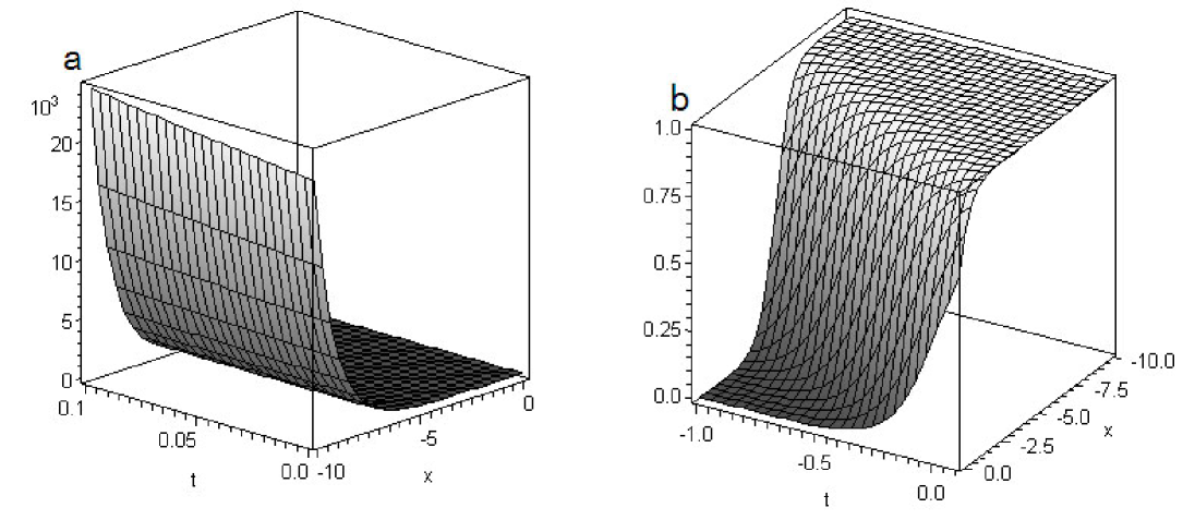
Figure 1: (a) Solution of Eq.(31) with $a_{0}=1$, $k=1$ and $\beta(t)=t$.   (b) Solution of Eq.(32) with $a=4$ and $c=5$.

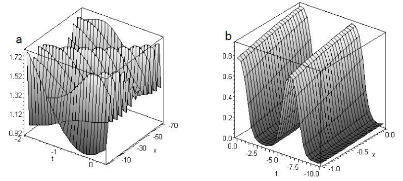
Figure 2: (a) Solution of Eq.(33) with $\beta(t)=\cos{t}$.   (b) Solution of Eq.(34) with $\beta(t)=-1+3\sin{t}$.

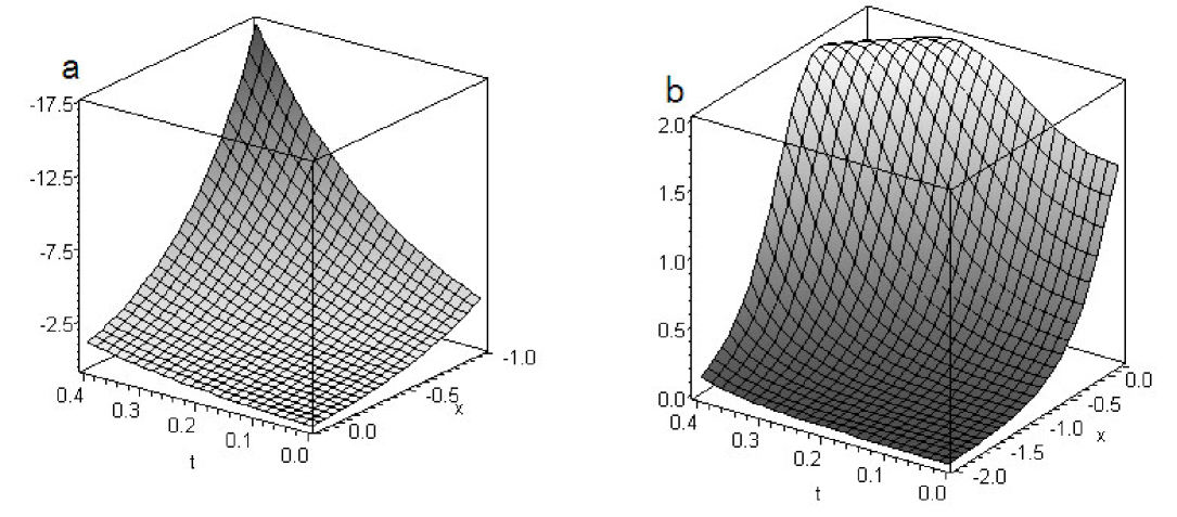
Figure 3: (a) Solution of Eq.(35) with $k=2$.  (b) Solution of Eq.(36) with $k=1$ and $b_{-1}=2$.

V conclusion

The Burgers-Fisher equation with variable coefficients is investigated by Exp-function method. The generalized Travelling wave solutions of this equation are obtained with the help of symbolic computation. From these results, we can see that the Exp-function method is one of the most effective methods to obtain exact solutions.

Finally, it is worthwhile to mention that the Exp-function method can be also extended to other nonlinear evolution equations with variable coefficients, such as the mKdV equation, the (3+1)-dimensional Burgers equation, the generalized Zakharov-Kuznetsov equation and so on. The Exp-function method is a promising and powerful new method for nonlinear evolution equations. This is our task in future work.

References

- (1) Abdusalam HA.On an improved complex tanh-function method. Int J Nonlinear Sci Numer Simul 2005; 6(2):99-106.
- (2) Zayed EME, Zedan HA, Gepreel KA. Group analysis and Modified extended tanh-function to fund the invariant solutions and soliton solutions for nonlinear Euler equations. Int J Nonlinear Sci Numer Simul 2004;5(3):221-34.
- (3) Bai CL, Zhao H. Generalized extended tanh-function method and its application. Chaos, Solutions & Fractals 2006;27(4):1026-35.
- (4) S.A.El-Wakil, M.A. Abdou. New exact travelling wave solutions using modified extended tanh-function method. Chaos, Solution & Fract.2007;31(4):840-852.
- (5) E.Fan,.Extended tanh-function method and its applications to nonlinear equations. Phys. Lett.A 2000;277:212-218.
- (6) Yomba E. The modified extended Fan sub-equation method and its application to the (2+1)-dimensional Broer-Kaup-Kupershmidt equation. Chaos ,Solitons & Fractals 2006;27(1):187-96.
- (7) Ren YJ, Zhang HQ. A generalized F-expansion method to find abundant families of Jacobi elliptic function solutions of the (2+1)-dimensional Nizhnik-Novikov-Veselov equation. Chaos ,Solitons & Fractals 2006;27(4):959-79.
- (8) A.M.Wazwaz. Exact solutions to the double sinh-Gordon equation by the separated ODE method. Comput. Math. Appl. 50(10-11)(2005)1685-1696.
- (9) C.Yan. A simple transformation for nonlinear waves, Phys. Lett. A 1996;246:77-84.
- (10) A.M. Wazwaz . A sine-cosine method for handing nonlinear wave equations. Math. Comput. Model.2004; 40:499-508.
- (11) Dai CQ, Zhang JF. Jacobian elliptic function method for nonlinear differential-difference equations. Chaos, Solitions & Fractals 2006;27(4):1042-7.
- (12) Zhao XQ,Zhi HY,Zhang HQ. Improved Jacobi-function method with symbolic computation to construct new double-periodic solutions for the generalized Ito system. Chaos, Solitions & Fractals 2006;28(1):112-26.
- (13) Yu Yx,Wang Q, Zhang HQ .The extended Jacobi ellipitic function method to solve a generalized Hirota-Satsuma coupled KdV equations . Chaos, Solitions & Fractals 2005;26(5):1415-21.
- (14) E.Fan, J Zhang. Applications of the Jacobi elliptic function method to special-type nonlinear equations. Phys. Lett. A 305(2002)383-392.
- (15) He JH, Application of homotopy perturbation method to nonlinear wave equations. Chaos, Solitons & Fractals 2005;26(3):695-700.
- (16) He JH. Homotopy perturbation method for bifurcation of nonlinear problems. Int J Nonlinear Sci Numer Simul 2005;6(2):207-8.
- (17) El-Shahed M. Application of He’s Homotopy perturbation method to Volterra’s integro-differential equation. Int J Nonlinear Sci Numer Simul 2005;6(2):163-8.
- (18) J.H.He. New interpretation of homotopy-perturbation method . Int.J.Mod.Phys.B 2006;20(18):2561-2568.
- (19) J.H.He. Some asymptotic methods for strongly nonlinear equations. Int.J.Mod.Phys.B 2006;20(10):1141-1199
- (20) J.H.He, X.H.Wu. Construction of solitary solution and compacton-like solution by variational iteration method. Chaos, Soliton & Fractals.2006; 29(1):108-113
- (21) Abassy TA, El-Tawil MA, Saleh HK, The solution of KdV and mKdV equations using Adomian Pade approximation. Int J Nonlinear Sci Numer Simul 2004;5(4):327-39.
- (22) El-Sayed SM, Kaya D, Zarea S. The decomposition method applied to solve high-order linear Volterra-Fredholm integro-differential equations. Int J Nonlinear Sic Numer Simul 2004;5(2):105-12.
- (23) El-Danaf TS,Ramadan MA, Alaal FEIA. The use of adomian decomposition method for solving the regularized long-wave equation .Ghaos, Solitons & Fractals 2005;26(3):747-57.
- (24) J.H.He,X.H.Wu. Exp-funtion method for nonlinear wave equations. Phys. Lett. A 2006; 30:700-708.
- (25) J.H.He, M.A.Abdou. New periodic solutions for nonlinear evolution equations using Exp-function method. Chaos Solitons & Fractals 2007;34(5):1421-1429.
- (26) Changbum Chun. Solitions and periodic solutions for fifht-order KdV eqaution with the Exp-function method. Phys.Lett.A 2008; 372:2760-2766.
- (27) Alvaro H.Salas. Exact solutions for the general fifth KdV equation by the exp function method. Appl.Math.Comput 2008;205: 291-297.
- (28) A. N. Kolmogorov, I. G. Petrovskii, and N. S. Piskunov. Investigation of the diffusion equation with growth of the quantity of matter and its application to a biology problem , Byull. Moskov. Gos. Univ. Mat. Mekh. 1 (1937), no. 6, 1 C26; English transl., Dynamics of curved fronts (P. Pelc e, ed.), Acad. Press, Boston 1988,pp 105 C130.
- (29) M. J. Ablowitz and A. Zeppetella. Explicit solutions of Fisher’s equation for a special wave speed. Bull. Math. Biol. 1979;41:835-840.
- (30) Jiang Lu, Guo Yu-Cui,Xu Shu-Jiang.Some new exact solutions to the Burgers CFisher equation and generalized Burgers CFisher equation. Chin. Phys. Soc.2007;16(09):2514-09.