Zero-point quantum fluctuations and dark energy
Abstract
In the Hamiltonian formulation of General Relativity the energy associated to an asymptotically flat space-time with metric is related to the Hamiltonian by , where the subtraction of the flat-space contribution is necessary to get rid of an otherwise divergent boundary term. This classic result indicates that the energy associated to flat space does not gravitate. We apply the same principle to study the effect of zero-point fluctuations of quantum fields in cosmology, proposing that their contribution to the cosmic expansion is obtained computing the vacuum energy of quantum fields in a FRW space-time with Hubble parameter and subtracting from it the flat-space contribution. Then the term proportional to (where is the UV cutoff) cancels and the remaining (bare) value of the vacuum energy density is proportional to . After renormalization, this produces a renormalized vacuum energy density , where is the scale where quantum gravity sets is, so for of order of the Planck mass a vacuum energy density of the order of the critical density can be obtained without any fine tuning. The counterterms can be chosen so that the renormalized energy density and pressure satisfy , with a parameter that can be fixed by comparison to the observed value, so in particular one can chose . An energy density evolving in time as is however observationally excluded as an explanation for the dominant dark energy component which is responsible for the observed acceleration of the universe. We rather propose that zero-point vacuum fluctuations provide a new subdominant “dark” contribution to the cosmic expansion that, for a UV scale slightly smaller than the Planck mass, is consistent with existing limits and potentially detectable.
I Introduction
The cosmological constant problem is a basic issue of modern cosmology (see e.g. Weinberg:1988cp ; Peebles:2002gy ; Padmanabhan:2002ji ; Copeland:2006wr ). One aspect of the problem is to understand what is the effect of the zero-point fluctuations of quantum fields on the cosmic expansion. Zero-point quantum fluctuations seem to give a contribution to the vacuum energy density of order , where is the UV cutoff. Even for a cutoff as low as , corresponding to scales where quantum field theory is well tested, this exceeds by many orders of magnitude the value of the critical density of the universe, which is of order . This aspect of the problem has by now a long history, which even goes back to works of Nernst and of Pauli in the 1920s Peebles:2002gy .
It is clear that this contribution should somehow be subtracted. Renormalization in quantum field theory (QFT) offers a logically viable possibility. One should not forget, in fact, that this cutoff-dependent contribution, as any similar quantity in QFT, is just a bare quantity rather than a physical observable. Working for instance with a cutoff in momentum space one finds that, in Minkowski spacetime, the bare, cut-off dependent, contribution to the vacuum energy density is
| (1) |
with some constant that depends on the number and type of fields of the theory. The standard procedure in QFT is to add to it a cutoff-dependent counterterm, chosen so that it cancels the divergent part and leaves us with the desired finite part (for an elementary discussion of this point in the cosmological constant case, see e.g. the textbook Maggiore:2005qv ), i.e.
| (2) |
where is independent of the cutoff and equal to the observed value of the vacuum energy density (assuming that vacuum energy is indeed responsible for the observed acceleration of the universe). The physical, renormalized, vacuum energy density
| (3) |
is therefore by definition independent of the cutoff and equal to the observed value . In principle this procedure is not different from what is done when one renormalizes, say, the electron mass or the electron charge in QED, where again with suitable counterterms one removes the divergent, cut-off dependent, parts and fixes the finite parts so that they agree with the observed values (in this sense the statement, often heard, that QFT gives a wrong prediction for the cosmological constant, is not correct. Strictly speaking QFT makes no prediction for the cosmological constant, just as it does not predict the electron mass nor the fine structure constant).
Still, for the vacuum energy this procedure is not really satisfying. The source of uneasiness is partly due to the fact that the counterterm must be fine tuned to a huge precision in order to cancel the term and leave us with a much smaller result. In fact, if in eq. (1) we take at least larger than a few TeV, where quantum field theory has been successfully tested, is at least of order , so in eq. (3) must be fine tuned so that it cancels something of order , leaving a result of order . This fine tuning becomes even much worse if one dares to take of the order of the Planck mass GeV. The fact that the counterterm must be tuned to such a precision creates a naturalness problem. Here, however, one might argue that neither the bare term nor the counterterm have any physical meaning and only their sum is physical, so this fine tuning is different from an unplausible cancellation between observable quantities. The same kind of cancellation appears, for instance, when one computes the Casimir effect. The crucial point, however, is that this renormalization procedure leaves us with no clue as to the physical value that emerges from this cancellation, so it gives no explanation of why the energy density associated to the cosmological constant appears to have just a value of the order of the critical density of the universe at the present epoch.
The point of view that we develop in this paper is that, even if renormalization must be an ingredient for understanding the physical effects of vacuum fluctuations, it is not the end of the story. The Casimir effect mentioned above gives indeed a first hint of what could be the missing ingredient for a correct treatment of vacuum energies in cosmology. In the Casimir effect the quantity that gives rise to observable effects, which have indeed been detected experimentally, is the difference between the vacuum energy in a given geometry (e.g., for the electromagnetic field, between two parallel conducting plates) and the vacuum energy computed in a reference geometry, which is just flat space-time in an infinite volume. Both terms are separately divergent as , but their difference is finite and observable. This can suggest that, to obtain the physical effect of the vacuum energy density on the expansion of the universe, one should similarly compute the vacuum energy density in a FRW space-time and subtract from it the value of a reference space-time, which is naturally taken as Minkowski space.
A possible objection to this procedure could be that General Relativity requires that any form of energy should be a source for the gravitational field, which seems to imply that even the vacuum energy associated to flat space should contribute. A more careful look at the formalism of GR shows however that the issue is not so simple and that, in a sense, the subtraction that we are advocating is in fact already part of the standard tenets of classical GR. To define carefully the energy associated to a field configuration in GR, it is convenient to use the Hamiltonian formulation, which goes back to the classic paper by Arnowitt, Deser and Misner ADM (ADM). As we will review in more detail in Section II, in order to define the Hamiltonian of GR one must at first work in a finite three-dimensional volume, and then the Hamiltonian takes the form
| (4) |
where is given by an integral over the three-dimensional finite spatial volume at fixed time, and by an integral over its (two-dimensional) boundary. At this point one would like to define the energy of a classical field configuration as the value of this Hamiltonian, evaluated on the classical solution, but one finds both a surprise and a difficulty. The “surprise” (which actually is just a consequence of the invariance under diffeomorphisms) is that , evaluated on any classical solution of the equations of motion, vanishes, so the whole contribution comes from the boundary term. The difficulty is that the boundary term, evaluated on any asymptotically flat metric (including flat space-time) diverges when the boundary is taken to infinity. The solution proposed by ADM is to subtract from this boundary term, evaluated on an asymptotically flat space-time with metric , the same term computed in flat space-time. The corresponding energy (or mass) is finite and is known as the ADM mass, and provides the standard definition of mass in GR. For instance, when applied to the Schwarzschild space-time, the ADM mass computed in this way turns out to be equal to the mass that appears in the Schwarzschild metric.
The ADM prescription can be summarized by saying that, in GR, the energy associated to an asymptotically flat space-time with metric can be obtained from the Hamiltonian by
| (5) |
where is the flat metric. Even if the context in which this formula is valid, namely asymptotically flat space-times, is different from the cosmological context in which we are interested here, still eq. (5) suffices to make the point that the intuitive idea that GR requires that any form of energy acts as a source for the gravitational field is not really correct. Equation (5) tells us that the energy associated to Minkowski space does not gravitate.
The idea of this paper is to generalize eq. (5) to the case of zero-point quantum fluctuation in curved space, proposing that the effect of zero-point fluctuations on the cosmic expansion should be obtained by computing the vacuum energy of quantum fields in a FRW space-time with Hubble parameter and subtracting from it the flat-space contribution. Computed in this way, the physical effect of zero-point fluctuations on the cosmic expansion can be seen as a sort of “cosmological Casimir effect”: while in the standard Casimir effect one computes the vacuum energy in a given geometry (say, for the electromagnetic field, between two infinite parallel conducting planes) and subtracts from it the value computed in a reference geometry (flat space-time in an infinite volume), here we compute the vacuum energies of the various fields in a given curved space-time, e.g. in FRW space-time, and we subtract from it the value computed in a reference space-time, i.e. Minkowski.
A possible objection to the idea of applying eq. (5) to vacuum fluctuations could be that one might think that, after all, the structure of UV divergences is determined by local properties of the theory, while whether a space-time is Minkowski is a global question. However one should keep in mind that, even if is a local quantity, the vacuum expectation value in a curved background involves the global aspects of the space-time in which it is computed. This is due to the fact that requires a definition of the vacuum state . The vacuum is defined from the condition , where the annihilation operators are defined with respect to a set of mode functions . The mode functions, in turn, are obtained solving a wave equation over the whole space-time, and therefore are sensitive to global properties of the space-time itself. In particular, in a FRW background the mode functions depend on the scale factor so their time derivatives (which enter in the computation of ) depend on the Hubble parameter . As we will review below, this results in the fact that the quadratic divergence in depends on the expansion rate of the FRW background.
The paper is organized as follows. In Section II we recall how eq. (5) is derived in the ADM formalism. The reader familiar with the subject, or not interested in the derivation, might simply wish to move directly to Section III, where we apply this classical subtraction, together with standard renormalization theory, to zero-point vacuum fluctuations. Some cosmological consequences of our proposal are discussed in Section IV, while Section V contains our conclusions.
II Subtractions in classical GR: the ADM mass
In this section we briefly discuss how the Arnowitt-Deser-Misner (ADM) mass is defined in GR ADM (we follow the very clear discussion of the textbook pois04 ). We begin by recalling that, in a finite four-dimensional volume with boundary , the gravitational action is (setting and using the signature )
| (6) |
where is the four-dimensional metric, is the metric induced on the boundary , , is the trace of the extrinsic curvature of the boundary, are the coordinates of the boundary, and on the regions of the boundary where is time-like and where is space-like. The first term is the usual Einstein-Hilbert action, while the second is a boundary term which is necessary to obtain a well-defined variational principle.
To pass to the Hamiltonian formalism one performs the decomposition of the metric,
| (7) |
where and are the lapse function and shift vector, respectively, and is the induced metric on the 3-dimensional spatial hypersurfaces. One defines as usual the conjugate momentum , where is the “volume part” of the Lagrangian density, and the Hamiltonian is then the volume integral of the Hamiltonian density . The explicit computation (see e.g. Section 4.2.6 of pois04 ) gives
where denotes the three-dimensional spatial hypersurfaces at fixed and (with coordinates ) is the intersection of with . In an asymptotically flat space-time is just a 2-sphere at large radius and fixed ; and depend only on and on its derivatives, but not on and , while in eq. (II) is the trace of the extrinsic curvature of , and is the determinant of the two-dimensional induced metric.
One would like to define the energy of a classical field configuration, i.e. of a solution of the equations of motion, as the value of this Hamiltonian on the solution. Performing the variation with respect to and one obtains the constraint equations and . Therefore, on a classical solution, the volume term in eq. (II) vanishes, and only the boundary term contributes. The ADM mass is defined by setting and after performing the variation (corresponding to the fact that energy is associated to asymptotic time translations; setting and one rather obtains the ADM momentum ), so only the term proportional to contributes to the mass. However, even for Minkowski space, this boundary term diverges. In fact, for an asymptotically flat space-time we can take to be a three-dimensional cylinder made of the two three-dimensional time-like hypersurfaces and (the “faces” of the three-dimensional cylinder) and of the space-like hypersurface . Let us denote by the extrinsic curvature of computed with a flat Minkowski metric. The faces at and have ; however, on the surface the extrinsic curvature is , while and , so the boundary term in eq. (7) is pois04
| (9) |
and diverges both when and when . As a consequence, also the boundary term proportional to in eq. (II) diverges, already for the Minkowski metric, and then of course also for generic asymptotically flat space-times. The ADM prescription is then to replace in eq. (6) by , i.e. to subtract from the trace of the extrinsic curvature computed with the desired metric, the value computed in flat space. Correspondingly, the trace of the two-dimensional extrinsic curvature in eq. (II) becomes , and the ADM mass of an asymptotically flat space-time is defined as ADM
| (10) |
If for instance one applies this definition to the Schwarzschild space-time, one finds that is equal to the mass which appears in the Schwarzschild metric.
What we learn from this is that, in classical GR, the mass or the energy that acts as the source of curvature of space-time, such as for instance the mass that enters in the Schwarzschild metric, can be obtained from a Hamiltonian treatment only after subtracting a flat-space contribution that need not be zero, and is in fact even divergent, but still does not act as a source of curvature.
III Application to zero-point energies
It is natural to apply the same principle to zero-point quantum fluctuations. In particular, in a cosmological setting, we propose that the zero-point energy density and pressure that contribute to the cosmological expansion are obtained by computing the energy density and pressure due to zero-point quantum fluctuations in a FRW metric with Hubble parameter , and subtracting from it the flat-space contribution.
We consider first the contribution of a real massless scalar field. In a FRW background the mode expansion of the field is
| (11) |
where is the comoving momentum, and satisfies the massless Klein-Gordon equation in a FRW background,
| (12) |
where the prime is the derivative with respect to conformal time . Writing this equation is reduced to the form
| (13) |
In a De Sitter background we have so , while in a matter-dominated (MD) epoch and therefore again . Thus, in both cases the positive frequency solution of eq. (13) is
| (14) |
and therefore is given by
| (15) |
with the scale factor of De Sitter or MD epoch, respectively. In contrast, during a radiation-dominated (RD) epoch , so . Then and
| (16) |
Using the energy–momentum tensor of a minimally coupled massless scalar field,
| (17) |
and setting , a simple computation Parker:1974qw ; Fulling:1974zr , reviewed in Appendix A, shows that the off-diagonal elements of vanish, while the vacuum energy density and pressure are given by
| (18) | |||||
| (19) |
where the dot denotes the derivative with respect to cosmic time . As they stand, these expressions must still be regularized, and we regularize them by putting a cutoff in momentum space. Recall that the comoving momentum is just a label of the Fourier mode under consideration, while the physical momentum of the mode is given by . We expect that quantum gravity enters the game when the physical momenta exceed the Planck scale, and we therefore put a time-independent cutoff over physical, rather than comoving, momenta. In terms of comoving momentum this means . Since the modes depend only on , the angular integrals are trivially performed, and we finally get
| (20) | |||||
| (21) |
III.1 Vacuum fluctuations in De Sitter space
III.1.1 Vacuum energy density
We compute first these expressions in De Sitter space. We therefore plug eq. (15), with , into eqs. (20) and (21). For the energy density the result is
| (22) | |||||
The first term is the well known flat-space result, proportional to the fourth power of the cutoff, while the term quadratic in is the correction due to the expansion of the universe. The appearance of a term , in a theory with two scales, the UV cutoff and the Hubble scale , can also be understood using rather general arguments Padmanabhan:2004qc .
According to our proposal we now subtract the flat-space contribution, which is simply the term in eq. (22), and we find that in De Sitter space the zero-point quantum fluctuations of a real scalar field have a (bare) energy density
| (23) |
The subscript “bare” stresses that this is still a bare, cut-off dependent quantity. We have eliminated the quartic divergence thanks to the “classical” prescription (5), but the result is still a bare energy density, diverging quadratically with the cutoff. In this sense, the situation is different from the usual Casimir effect, where the subtraction of the flat-space contribution suffices to make the result finite. However, we can now use standard renormalization theory, so the renormalized energy density is obtained by adding a counterterm whose divergent part is chosen so to cancel this quadratic divergence, and whose finite part is in principle fixed by the observation, so
| (24) |
As usual in the renormalization procedure, the finite part cannot be predicted. It must be fixed to the observed value. What we have gained, with respect to eq. (2), is that now we have a different understanding of what is a “natural” value of this finite part. If quantum gravity sets in at a mass scale (so that could be typically given by the Planck mass , or by the string mass), a natural, non fine-tuned value of is given by
| (25) |
where “” is a constant , which cannot be fixed by naturalness arguments only, and must be determined by comparison with the experiment.111More precisely, renormalization trades the cutoff for the subtraction point . While the latter is in principle arbitrary, a clever choice of will minimize the effect of radiative corrections. For instance, if one renormalizes the electroweak theory in the MS scheme, one naturally takes . Using a much lower subtraction point, say , is in principle legitimate, but all radiative corrections would then become large, and the whole perturbative approach could be spoiled. In this sense, is a natural subtraction point for the electroweak theory, and we similarly expect that, in a theory involving quantum gravity, the natural subtraction point will be given by the Planck or string mass. (I thank a referee for this comment).
Observe that naturalness arguments cannot fix the sign of the finite part either, and we have added a factor to take this fact explicitly into account. There is in fact no a priori reason why the renormalized vacuum energy should necessarily be positive. For instance, the vacuum energies obtained for fields in a finite volume from the Casimir effect can be either positive or negative, depending e.g. on the type of field and on the geometry considered.
III.1.2 Equation of state and general covariance
Repeating the same computation for the pressure we get
| (26) | |||||
The term in eq. (26) was already computed in Akhmedov:2002ts and is just the result in Minkowski space, that we subtract, so we end up with
| (27) |
Observe that . However, it would be incorrect to conclude that vacuum fluctuations in De Sitter space satisfy the equation of state with . The point is that this relation only holds for the bare quantities, and not necessarily for the renormalized ones. The physical, renormalized, pressure is obtained by adding a counterterm
| (28) |
Observe that regularizing the theory with a cutoff over spatial momenta, as we have done, breaks explicitly Lorentz invariance in Minkowski space, since the notion of maximum value of spatial momenta is not invariant under boosts. In a generic FRW background, of course, Lorentz transformations are not a symmetry of the theory, since the metric depends explicitly on time, and the guiding principle is rather general covariance, which again is broken by a cutoff over spatial momenta. However, even if the regularization breaks general covariance, in De Sitter space a generally covariant result can still be obtained in the end for the physical, renormalized, vacuum expectation value of the energy-momentum tensor, just by choosing the finite parts of the counterterms such that . Then the vacuum expectation value of the renormalized energy-momentum tensor becomes
| (29) |
or, lowering the upper index with the metric ,
| (30) |
Since in De Sitter space is constant we see that, with the choice , is just given by a numerical constant times , and it is therefore covariantly conserved. In the language of the effective action for gravity, which is obtained by treating the metric as a classical background and integrating over the matter degrees of freedom (see e.g. refs. Barvinsky:1985an ; Buchbinder:1992rb ; Shapiro:2008sf ), the vacuum expectation value of the energy-momentum tensor is given by the functional derivative of the effective action. Then a contribution such as that given in eq. (30) can be obtained by taking the functional derivative of the volume term in the effective action (see ref. Pelinson:2010yr for a discussion of the equation of state that can be obtained from the various contributions to the effective action).
The choice will therefore be assumed in the following, for De Sitter space-time. Observe that a covariant result for the renormalized value of is obtained with a counterterm that is not covariant, i.e. is not proportional to , since , but again this is a consequence of the fact that our regularization is not covariant.
III.1.3 Contribution of higher-spin fields and massive particles
A similar conclusion about the “natural” value of the energy density of vacuum fluctuations holds if we add the contribution of fields with different spin. In fact, massless fermions and gauge bosons have a conformally invariant action and then, since the FRW metric is conformally equivalent to flat Minkoswki space, their vacuum energy in a FRW space-time is the same as in Minkowski space. Therefore, with our subtraction (5), they do not contribute to and . This is completely equivalent to the well known fact that vacuum fluctuations of massless fermions and gauge bosons are not amplified during inflation.
The contribution of massive fermions to vacuum fluctuations in De Sitter space, as well as the generalization of eq. (22) to massive bosons, can be readily computed. For massive bosons, eq. (22) becomes Fulling:1974zr ; Bilic:2010xd
| (31) |
where we have neglected terms of order , and terms convergent in the UV; is defined as
| (32) |
so in the massless limit and we recover eq. (22) 222Observe that in ref. Bilic:2010xd the result is written directly for the complex scalar belonging to a chiral superfield, hence the bosonic vacuum energy in eq. (32) of ref. Bilic:2010xd is twice as large as that in our eq. (22), which holds for a real scalar field.. In this massive case our prescription amounts to subtracting the flat-space contribution given by the term in brackets. The remaining, quadratically divergent term, leads again to eq. (25), times a correction , and to a logarithmically divergent term, which after renormalization produces a contribution to proportional to , and therefore subleading for .
The contribution of a massive Majorana spinor field to the vacuum energy density in De Sitter space is instead Bilic:2010xd
| (33) |
The first term in brackets gives the usual negative contribution to vacuum energy in flat space due to fermions. Observe that in a supersymmetric model, where to each Majorana spinor is associated a complex scalar field, and therefore two real scalar fields, the contribution in eq. (33) cancels exactly the bosonic contribution in eq. (31), giving the usual cancellation of vacuum energy for a supersymmetric theory in Minkowski space. In a realistic model with supersymmetry broken at a scale , this cancellation is however only partial and leaves the usual result of order . In our approach, instead, the quartic divergence are eliminated exactly by the prescription of subtracting the flat-space contribution.
The term that remains in eq. (33), after subtraction of the flat-space contribution, gives a divergent contribution equal to (consistently with the fact that, for , it must vanish because of conformal invariance). After renormalization, this gives a contribution to the vacuum energy which is of order , and which therefore for , is negligible with respect to the bosonic contribution (25). It is also interesting to observe that, even in a theory with exact supersymmetry, the cancellation between fermionic and bosonic divergences only takes place at the level of the quartic divergence. There is no contribution proportional to from the fermionic sector, and therefore the whole contribution proportional to comes from the bosonic sector. This means that eq. (25) holds even in a theory with exact or broken supersymmetry.
In contrast, gravitons give a contribution to the bare energy density proportional to . In fact, in a FRW space-time each of the two helicity modes , with satisfies separately the same wave equation as eq. (12) with replaced by ,
| (34) |
So each of the two helicity modes gives the same contribution to and as a minimally coupled massless scalar field. Therefore, in a theory with minimally coupled elementary scalar fields plus the two degrees of freedom for the graviton, the natural value for the energy density, eq. (25), is of order . In particular, even in a theory with no fundamental scalar field, a contribution of order comes anyhow from gravitons.
III.2 Vacuum fluctuations during RD and MD
It is straightforward to repeat the same calculation for a radiation-dominated (RD) and for a matter-dominated (MD) era. For the RD epoch we use the modes (16). Then, recalling that ,
| (35) |
where as usual the dot denotes the derivative with respect to cosmic time and the prime the derivative with respect to . Using , we get
| (36) | |||||
so the energy density turns out to be identical to eq. (22), except that now is replaced by . For the pressure we get
| (37) |
Thus, once removed the Minkowski term, we remain with
| (38) |
while for the pressure we get . Similarly to what we have discussed in the de Sitter case, this means that the natural value of the renormalized energy density is
| (39) |
where is the scale where quantum gravity sets in, “” is a numerical constant , and . On the other hand, the relation does not imply that the renormalized energy density and the renormalized pressure satisfy an equation of state with . As in the de Sitter case, the finite part in the counterterm for the pressure can be chosen so to reproduce any observed value of , in particular the value . The issue of general covariance is however now more subtle, since even the choice now leads to
| (40) |
which, because of the time dependence of , is no longer covariantly conserved. However, general covariance actually only requires that the total energy momentum tensor, including that of matter, radiation, etc., be covariantly conserved. The fact that energy-momentum tensor associated to vacuum fluctuations is not separately conserved means that there must be an energy exchange between vacuum fluctuations and other energy sources such as radiation or matter, so that we are actually dealing with an interacting dark energy model. We will come back to this issue in Section IV.
For MD we use the modes given in eq. (15), with . For the energy density we find
| (41) |
So, both for MD and for RD, the first two terms are the same as in De Sitter, eq. (22), except that becomes . Again, the first term is the Minkowski contribution, that we subtract. The term diverges only logarithmically with the UV cutoff (and also require an IR cutoff, which for a light scalar field is provided by its mass, while for a strictly massless field could be taken equal to ). Thus, for the physical, renormalized, energy density we find again that the natural value is given by eq. (39), since the term in eq. (41) produces a subleading term of order .
Recalling that (in units ) Newton’s constant is , and that the critical density at time is
| (42) |
we can express the above result by saying that the “natural” value suggested by QFT is
| (43) |
with and . We therefore find that, both during RD and MD, the renormalized energy density due to zero-point quantum fluctuations is not a constant, and therefore does not contribute to the cosmological constant. Rather, it is a fixed fraction of the critical density .
As before, each helicity mode of a graviton contributes as a minimally coupled scalar field, while gauge bosons do not contribute and the contribution of light fermions is suppressed by a factor . Thus, in a theory with fundamental minimally coupled scalar fields plus the two helicity modes of the graviton we have, for either De Sitter, RD or MD,
| (44) |
where the subscript stands for “zero-point quantum fluctuations”, and the natural value of is
| (45) |
where is the scale where quantum gravity sets in, e.g. itself or the string scale. As we have seen in eqs. (31) and (33), bosons or fermions with mass not far from the quantum gravity scale would give corrections of order to this estimate (which could become numerically important if there were, e.g. many fermions at a scale, such as the GUT scale, not far from the Planck mass). The computation of the pressure during MD gives
| (46) |
Again, the first term is the Minkowski contribution, that we subtract, and we neglect the term . Thus, we finally find
| (47) |
and therefore, during MD, , but again the renormalized energy and pressure satisfy with determined by the observation.333It is curious to observe that in all three case (De Sitter, RD and MD) the bare quantities and satisfy with where is the -parameter of the component that dominates the evolution during the corresponding phase, i.e. during De Sitter, RD and MD, respectively.
A technical point that deserves some comment is the choice of the modes given in eqs. (15) and (16). These modes are particularly natural since in the UV limit they reduce to positive-frequency plane waves in flat space. However, the choice of the modes is equivalent to the choice of a particular vacuum state, and the most general possibility is a superposition of positive- and negative-frequency modes with Bogoliubov coefficients and . As we show in appendix B, for a generic choice of vacuum the dependence of the natural value of on is not altered, while the numerical coefficient in front of it can change.
A conceptually interesting aspect of the result (39) is that it appears to involve a mixing of ultraviolet and infrared physics, since it depends both on the UV scale , and on the horizon size , which represents the “size of the box”, and therefore plays the role of an IR cutoff. This is an interesting result by itself, since in quantum field theory we are rather used to the fact that widely separated energy scales decouple. Observes that this UV-IR mixing comes out only because our classical subtraction procedure based on eq. (5) eliminates the troublesome term diverging as , which is instead a purely UV term. As we already discussed in the Introduction, the origin of this UV-IR mixing can be traced to the fact that, even if is a local quantity, the vacuum expectation value is sensitive to through the definition of the vacuum state . In fact, the vacuum is defined from the condition , where the annihilation operators are defined with respect to a set of mode functions ; these mode functions are obtained solving a wave equation over the whole space-time, and therefore are sensitive to the time evolution of the scale factor and, more generally, to the overall geometry of space-time.
IV Cosmological implications
IV.1 Vacuum fluctuations and the dominant component of dark energy
The results of the previous section show that, with the subtraction that we advocate, zero-point vacuum fluctuations do not contribute to the cosmological constant since their energy density, given in eqs. (44) and (45), is not a constant, but rather a fixed fraction of the critical energy at any epoch.
The first question to be addressed is whether a vacuum energy density with such a time behavior could be identified with the dark energy component which is responsible for the observed acceleration of the universe. If this were the case, since we have found that the vacuum energy density scales as , we would have where we follow the standard use of denoting by the value of at the present time . Such a model has been compared to CMB+BAO+SN data in ref. Basilakos:2009wi , where it is found that it is ruled out at a high significance level.
Formally the result of ref. Basilakos:2009wi comes from the fact that the obtained fitting this model to the usual estimators for CMB, for BAO and to SNIa turns out to be unacceptably high. However, independently of technical details, it is easy to understand physically why such a model for dark energy is not viable. Consider in fact a spatially flat model with vacuum energy density evolving as , with equation of state , and matter density , with , in the recent universe where we can neglect . The total energy-momentum conservation is
| (48) |
and cannot be split into two separate conservation equations for and , and , since the second equation is obviously incompatible with , in the recent universe where the Hubble parameter is certainly not a constant. This means that energy must be transferred between and in order to obtain the behavior , so we have an interacting dark energy model. The Friedmann equation in this model reads
| (49) | |||||
and therefore
| (50) |
and
| (51) |
In this model, therefore, the time evolution of dark energy density is the same as that of matter. This is clearly incompatible with the existing cosmological observations, that rather indicate that in the recent epoch remained constant, at least to a first approximation, while the matter density in the concordance CDM model evolves in a way that cannot differ too much from . More quantitatively, combining the Friedmann equation (50) with the total energy-momentum conservation equation (48) it can be easily found Basilakos:2009wi that in this model the dependence of on the scale factor is
| (52) |
where we normalize the scale factor so that at the present epoch (we will see explicitly in Sect. IV.3 how to derive this result in a similar setting). Physically this result expresses the fact that in this model decreases with time, rather than remaining constant as it would do in isolation, and therefore part of its energy density must be transferred to matter, through the energy-conservation equation (48). So, matter energy density decreases more slowly that . For , recalling that we are considering a flat model with , eq. (51) gives
| (53) |
To compare these results to observations, we recall that the possibility of a time evolution of the dark energy density is usually studied in the literature by parametrizing it as
| (54) |
It is important to stress that eq. (54) is simply an effective way of parametrizing the time dependence of in order to compare it with the observations, and the parameter that appears there is equal to the parameter that enters in the equation of state of dark energy only if dark energy is not interacting which, as we have seen, is not the case for a model where .
Comparing eqs. (53) and (54) we see that a model with predicts that the effective parameter in eq. (54) is constant in time, and equal to . The limit on constant obtained from WMAP 7yr data+BAO+SN is at 68% c.l. Komatsu:2010fb (actually, this value does not include systematic errors in supernova data; including the systematics, the error on rather becomes about 0.08, see Amanullah:2010vv ), and therefore reproducing this value would require , and consistent with zero to a few percent! It is no wonder that such a model does not fit (any) other cosmological observation. Alternatively, setting and , we get a prediction , which is excluded at a high confidence level.
Therefore, it appears that the interpretation of zero-point quantum fluctuations as the dominant dark energy component, responsible for the acceleration of the universe, is not viable. In the next section we will explore the possibility that they could still provide a new, subdominant, “dark” component, that we will denote by to distinguish it from the dominant component which instead, according to the limits on , is at least approximately constant in time. We will see that, for plausible values of the mass scale where quantum gravity sets in, the energy density can have a value consistent with existing observations, but still potentially detectable.
IV.2 Theoretical expectations for
The effect of on the cosmological expansion depends on the mass scale , whose exact value can only be determined once one has a fundamental theory of quantum gravity. If we set and we consider the Standard Model with one Higgs field, so , eq. (45) gives . However, precise numerical factors are beyond such order-of-magnitude estimates and, by lowering the UV scale , it is easy to reduce this number to smaller but still potentially observable values. For instance, in heterotic string theory the scale is rather given by the heterotic string mass scale , where is the value of the gauge couplings at the string scale Antoniadis:1999cf . This would rather lead to the estimate . Lower values of the cutoff, possibly down to the TeV scale, can be obtained in theories with large extra dimensions ArkaniHamed:1998nn . It is also important to observe that, as explained in the discussion below eq. (33), the estimate given in eq. (45) holds even in a theory with exact or broken supersymmetry, since the contribution proportional to comes anyhow only from the bosonic sector.
IV.3 Cosmological evolution equations
We consider a flat CDM cosmology, with a vacuum energy having an equation of state and we further add the energy density given in eq. (44), with . We have nothing to add to the problem of the physical origin of , except that in our model it is not due to zero-point quantum fluctuations: it has nothing to do with the quartic divergence in the vacuum energy (which is eliminated by our ADM-like subtraction), nor with the quadratic divergence, which is instead the origin of . Then in this model (which could be conveniently called ZCDM)
| (55) | |||||
| (56) |
The values will be assumed in the following (in appendix C we discuss the case generic). From eq. (44),
| (57) |
where is the present value of the critical density, so the energy density in the dark sector is
| (58) | |||||
Quite interestingly, this is the same form of the dark energy density found in refs. Shapiro:2000dz ; Shapiro:2003ui ; EspanaBonet:2003vk ; Shapiro:2009dh from an apparently rather different approach, namely from the suggestion that the cosmological constant could evolve under renormalization group, after identifying their parameter with our , compare with eq. (13) of ref. Shapiro:2003ui . Observe also that their value for the parameter is where is the mass scale where new physics comes in. This has the same parametric dependence on as our result for , and is even quite close numerically 444Observe that the value of their numerical coefficients depends on the precise definition of the mass scale , which in the approach based on RG involves not only the UV scale, but also some unknown beta-function coefficients, see eqs. (3.6) and (4.2) of ref. EspanaBonet:2003vk ..
Using eq. (58), the Friedmann equation becomes
| (59) |
which can be rewritten as
| (60) |
where , (). Thus, the effect of on the Friedmann equation is equivalent to a rescaling of the present value of the Hubble constant, or, equivalently, to a rescaling of (with ) into . Even if we set we have for the moment written , rather than setting it to a constant, in order to allow for the possibility of an energy exchange between and , see below.
Zero-point fluctuations also contribute to the equation for the acceleration
| (61) |
in a way which depends on the sign of . With (or more generally whenever ), zero-point fluctuations contribute to accelerating the universe if , while for they give a contribution that decelerates the expansion, and which therefore opposes the accelerating effect of .
We next consider the energy conservation equation. As we already mentioned in Section III.2, the fact that zero-point quantum fluctuations have an energy density has non-trivial consequences on the conservation of energy. Consider in fact the energy conservation in a FRW background,
| (62) |
When there is no exchange of energy among the different components, energy conservation is satisfied separately for each component, so with . If this were the case, using , the equation
| (63) |
would give , and in particular constant if . However, we have found that . So, energy must be transferred between zero-point fluctuations and other components 555Unless evolves in time so to track the equation of state of the dominant energy component, i.e. it evolves from during RD to during MD. Another interesting possibility, that we do not consider here, is that the Bianchi identities are actually satisfied by assuming a standard conservation law for matter, but assigning a time dependence to Newton’s constant, see Sola:2007sv ..
In principle, there are various mechanisms by which vacuum fluctuations can exchange energy with ordinary matter. A typical example is the amplification of vacuum fluctuations Gri ; Star , or the change in a large-scale scalar field due to the continuous flow across the horizon of small-scale quantum fluctuations of the same scalar field, which is also at the basis of stochastic inflation Star2 . If we assume that exchanges energy with but not with the relevant conservation equation is (setting hereafter )
| (64) |
Using eq. (57), we then obtain
| (65) |
This equation was already discussed in refs. EspanaBonet:2003vk ; Basilakos:2009wi in the context of their time-varying cosmological constant model and, following these papers, to solve it we compute the term on the right-hand side by using the Friedmann equation (60) and we obtain (neglecting for simplicity in the low redshift epoch in which we are interested here)
| (66) |
where we used the fact that, since we are assuming that only interacts with , and we are furthermore assuming , the energy density evolves in isolation and satisfies . Equation (66) can be rewritten as
| (67) |
and has the solution
| (68) |
Of course, since we have taken , if vacuum energy density were non-interacting it would remain constant in time. In the case (i.e. when ) we have rather found that is proportional to , and therefore it decreases with time instead of staying constant. This means that dark energy is interacting, and that energy is transferred from vacuum fluctuations to matter, for instance with a mechanism analogous to the amplification of vacuum fluctuations, and as a result the energy density of matter must decrease slower than . This is reflected in eq. (68), since for we find that indeed decreases slower than . If the situation is reversed. A behavior means that becomes less and less negative as time increases, so energy is transfered from matter to vacuum fluctuations, and decreases faster than .
In the absence of an understanding of the dynamical origin of the dominant dark energy term , it is interesting to consider also the possibility that energy could be exchanged also between and . We assume at first, for simplicity, that energy is exchanged only with , and not with . Then the corresponding conservation equation (taking for simplicity) is
| (69) |
which trivially integrates to
| (70) |
and therefore, using ,
| (71) |
where, as usual, on the right-hand side . However, in terms of the total dark energy density defined in eq. (58), we see that in this case we simply have a total dark energy density that satisfies , while the matter energy density satisfies its usual conservation equation , and also eqs. (59) and (61), when rewritten in terms of , take the standard CDM form. Thus, in the end a model where only exchanges energy with (and in which ) is indistinguishable from standard CDM cosmology with just a cosmological constant. In the most general case in which , however, even setting the pressure is no longer equal to , so this model has observable deviations for CDM, and is in fact of the type called XCDM Grande:2006nn ; Grande:2006qi ; Grande:2008re ; Bauer:2010wj . In the following we will however restrict to .
A more general phenomenological analysis, in which one takes into account the possibility that interacts both with and with , can be performed by splitting the conservation equation
| (72) |
into the two equations
| (73) | |||||
| (74) |
where . Equation (64) corresponds to the limiting case while eq. (69) corresponds to the limiting case . Rewriting these equations in terms of the total dark energy density , we get
| (75) | |||||
| (76) |
which shows that the observable consequences depend only on the combination . In other words, as long as , there is no point in postulating an energy exchange between and , since only the fraction of which is exchanged with has observable consequences. In the following we will limit ourselves to , and we then set .
IV.4 Limits on from cosmological observations
In this section we perform a first analysis of the limits that some cosmological observations impose on . A more detailed comparison with the data will be presented elsewhere. The fact that the energy budget of the universe at the present epoch is known to a precision of about by itself does not yet constraint , since a part of what is normally attributed to could be due to . The only way of disentangling them is by using their different temporal evolution, since while the dominant component is constant, at least within the present experimental accuracy. In the next subsections we examine various limits on which make use of the time dependence .
IV.4.1 Bound on from BBN
We first examine the bound coming from big-bang nucleosynthesis (BBN), which constraints the energy budget of the universe at that epoch. The limit on extra contributions to the energy density at time of BBN is usually expressed in terms of the effective number of neutrino species , defined so that any extra source of energy density, compared to the Standard Model, is written as
| (77) |
and , where is the value predicted by the Standard Model with three light neutrino families, after taking into account finite temperature QED corrections and the fact that neutrino decoupling is not instantaneous Mangano:2005cc . The most recent BBN bound is at 95% c.l. Iocco:2008va , corresponding to a limit . At the epoch of BBN only the photons and the three neutrinos contribute significantly to the energy density, while already annihilated into photons, resulting in a photon temperature higher than the neutrino temperature by a factor . Therefore, at BBN,
| (78) |
where the factor comes from Fermi statistics. Combining this with eq. (77) gives
| (79) |
This gives a corresponding bound on the total dark energy density at the time of nucleosynthesis. From eq. (75) with we have , so
| (80) |
At the constant term in bracket is totally negligible with respect to the critical density , while , so the bound (79) translates into
| (81) |
Strictly speaking, BBN gives an upper bound only on , and not on its absolute value, since negative values of could in principle be compensated by other forms of energy.
IV.4.2 Bound on from CMB+BAO+SNIa
A comparison of this model to CMB+BAO+SNIa data has been performed in ref. Basilakos:2009wi within the context of the model of a cosmological constant that evolves under renormalization group Shapiro:2000dz ; Shapiro:2003ui ; EspanaBonet:2003vk ; Shapiro:2009dh . Even if our physical motivations are different from theirs, the model is phenomenologically the same, and our parameter corresponds to the parameter that they denote as (or as ). We can therefore translate immediately their result in our setting. In particular, from a joint analysis of CBM+BAO+SNIa, sampling the interval 666The analysis was actually restricted to positive values of (J. Solà, personal communication). in steps of 0.001, they find a best fit value .
IV.4.3 Bound on from the limits on the time evolution of dark energy
It is also instructive to compare the time evolution of a dark energy density of the form to the existing observational limit, which is also obtained from a combination of CMB+BAO+SNIa data.
In standard CDM cosmology, without the contribution , the dark energy density is given uniquely by and, allowing for a generic , its evolution with redshift is given by
| (82) |
while (neglecting , since we are interested here in the evolution at small redshifts) the critical density is given by
| (83) |
with . Then
| (84) |
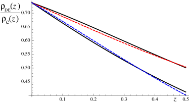
We use the recent determination of given in Amanullah:2010vv , at 68% c.l., which includes also systematic errors on supernova data (the more stringent bound given in Komatsu:2010fb only includes the statistical error in the SN data). In Fig. 1 we then plot the function given in eq. (84), in correspondence of the upper and lower limits on , and , respectively (black solid lines). We limit ourselves to the redshift interval that, as shown in Kowalski:2008ez ; Amanullah:2010vv , is responsible for most part of the bound on . Plotting the constraint on , or the corresponding constraints on , in different redshift bins, one finds in fact that the bin already gives a poorly constrained , see e.g. Fig. 15 of Amanullah:2010vv .
In this range of redshifts, we compare the temporal evolution given in eq. (84) with and with , respectively, to that obtained in ZCDM (using for definiteness the values ). From eq. (80),
| (85) |
where . To write explicitly the critical density we use the Friedmann equation (60) (neglecting again ) together with eq. (68), so
| (86) | |||||
and therefore, writing ,
| (87) |
Combining eqs. (85) and (87) we get
| (88) |
This function is plotted in Fig. 1, keeping fixed at the observed value , and choosing (upper dashed line, red) and (lower dashed line, blue). We see that, at least at this relatively crude level of analysis, values of in the approximate range are consistent with the observational limits on the temporal evolution of dark energy, since the corresponding curves stay inside the two curves with and , respectively, down to the maximum redshifts where is significantly constrained by the data. If one would rather compare the function given in eq. (84), to the upper and lower limits on and , one would rather find . Of course this analysis gives only a first rough but intuitive estimate of the bound that can be obtained from the limits on the redshift dependence of . A more accurate study requires fitting this model to the data, as in Basilakos:2009wi .
IV.5 How not to solve the cosmological constant problem
We think that another useful aspect of the above analysis is to put in a sharper focus where the main difficulty is, in explaining the observed value of dark energy density. If one looks at eq. (39), which holds both in RD and in MD, setting equal to the present time and , one finds that the energy density associated to vacuum fluctuations today is , which is of the right order of magnitude of the observed dark energy density (it could even be tempting to observe, from eqs. (44) and (45), that with , and one gets , which is very close to the measured value ). However, at this stage this observation is not yet a possible explanation of the numerical value of the cosmological constant, not even at the level of orders of magnitude. The trouble is that the same computation, performed at a generic time , gives , so the resulting energy density is not constant. As we have discussed in Section IV.1, such a time behavior is observationally excluded, at least for the dominant dark energy component, and can only be accepted for a suitably small subdominant dark component.
We should observe that the same conclusion also applies to some existing attempts at computing the cosmological constant which make use of and , such as the holographic approach to the cosmological constant Cohen:1998zx ; Hsu:2004ri ; Horvat:2004vn , where again one obtains a value of order today. However, the very same reasoning would give at a generic time, which as we have seen is ruled out, at least for the dominant component of dark energy.
A similar remark can also be made for the result of ref. Schutzhold:2002pr , where it is proposed that the trace anomaly in QCD gives a contribution to the vacuum energy density proportional to times the Hubble parameter to the first power. Using the present value of the Hubble parameter, ref. Schutzhold:2002pr finds that is roughly comparable to (actually, this is true only within about one or two orders of magnitude; for the typical values of , we get , not that close to . Of course precise numerical factor were anyhow beyond the estimate in ref. Schutzhold:2002pr ). In any case, the suggestion of ref. Schutzhold:2002pr that this effect has a potential relevance for explaining the observed acceleration of the universe faces a problem similar to the one discussed above. In fact, if at the present time one finds , the same calculation, performed at a generic time of course gives . As shown in ref. Basilakos:2009wi , this behavior is ruled out by the comparison with CMB+BAO+SNIa data. (It should also be observed that a contribution to the vacuum energy density proportional to an odd power of is not consistent with the general covariance of the effective action for gravity, see Section 3.1 of ref. Shapiro:2008sf ).
What we learn from the above examples is that the real challenge, in explaining the cosmological constant, is not so much to explain its numerical value today; having at our disposal the two scales and , once the term proportional to is eliminated one naturally remains with a result proportional to , which gives the right order of magnitude. The real challenge is to find a dynamical mechanism that gives a value of order today, without giving at a generic time , which is the essence of the coincidence problem.
V Conclusions
One aspect of the cosmological constant problem, or more generally of the problem of understanding the origin of dark energy, is to understand why zero-point fluctuations of quantum fields do not produce an energy density of the order of , where is the UV mass scale of the quantum field theory (e.g. the Planck mass, or the string mass scale), despite the fact that this seems to be the natural value suggested by quantum field theory. We have proposed that the solutions to this long-standing puzzle has a purely classical origin, and is related to the correct definition of energy in classical General Relativity, which already involves the subtraction of the flat-space contribution, see eq. (5).
We have applied this subtraction procedure to a FRW space-time with Hubble parameter and we have found that the remaining energy density, after renormalization, has a “natural” value proportional to (and a sign that could in principle be either positive or negative, just as in the Casimir effect). For this gives an energy density just of the order of the critical density of the universe. As we have discussed, however, such an energy density has a time dependence that is not compatible with present observations, if we identify it with the dark energy component with which in the standard CDM cosmology is responsible for the observed acceleration of the universe. It is however possible that it represents a new form of dark energy, whose normalized energy density today, , is smaller than . Values of are compatible with the observations that we have discussed, but could give observable effects in more detailed studies that make use of the specific signature of zero-point fluctuations, namely an energy density with a time dependence proportional to , as well as in future more accurate cosmological observations.
Acknowledgments. I thank Ruth Durrer, Juan Garcia-Bellido, Alberto Nicolis, Massimiliano Rinaldi, Antonio Riotto, Joan Solà and the referees for very useful comments on the manuscript. This work is supported by the Fonds National Suisse.
Appendix A Computation of and in FRW background
Even if the computation leading to eqs. (20) and (21) is elementary, we find it useful to report it here. The energy associated to a real massless scalar field in a FRW metric, in a comoving volume , is
| (89) | |||||
where we used from eq. (17). Observe that are comoving coordinates and the factor transforms the comoving volume element into the physical volume element. Using the mode expansion (11) we get, taking for illustration the term ,
Performing the integral in over a volume large compared to the wavelength of all modes of interest we have
| (90) |
and we get
| (91) | |||||
Observe that in flat Minkowski space and (since we are considering a massless field) , so the term proportional to vanishes. In a generic curved space it is instead non-zero, so a general state in a curved background is characterized by the expectation values and Parker:1974qw . For the vacuum state, however, the only non-vanishing contribution comes from the term proportional to in eq. (91), and can be computed using , from which it follows that , where is the comoving spatial volume (since is a comoving momentum), and therefore
| (92) |
Multiplying the comoving volume by the factor we recover the physical volume , and therefore the energy of zero-point quantum fluctuations is
| (93) |
The vacuum energy density is then defined as .
For the pressure, the spatial isotropy of the FRW metric implies that (observe that, with our signature the energy-momentum tensor of a perfect fluid is ). It is convenient to write and, as we have done for the energy density, consider first the integrated quantity
where, in the second line, the sum over is understood. Repeating the same steps as above, we get the zero-point contribution
| (95) |
and . The off-diagonal elements of the volume integral of vanish trivially, since they involves integrations over , or over with , which vanish by parity.
Appendix B Dependence on the choice of vacuum
A point that deserves some comment is the choice of the modes given in eqs. (15) and (16). These modes are particularly natural since in the UV limit they reduce to positive-frequency plane waves in flat space. However, the choice of the modes is equivalent to the choice of a particular vacuum state, and the most general possibility is a superposition of positive- and negative-frequency modes (15), (16) with Bogoliubov coefficients and ,
| (96) |
where for RD and for De Sitter and MD, and the Bogoliubov coefficient satisfy the normalization condition . It is straightforward to repeat the computation of the vacuum energy density using the modes (96). When computing and , mixed term proportional to and to have a time dependence which contains the factors . After integrating over these produce terms proportional to and . Since
| (97) |
these terms oscillate very fast in time, with a Planckian frequency, and therefore they average to zero over any macroscopic time interval, and can be dropped. Keeping only the contributions proportional to and to , subtracting as usual the Minkowski term (and neglecting again the term which appears in the MD case), for a real scalar field we find
| (98) |
and , where is the same found before. Therefore a different choice for the vacuum affects the numerical value of in eq. (44) by a numerical factor which reflects the occupation number of the various modes.
Appendix C Cosmological equations for generic
In Section IV.3 we studied the cosmological evolution equations setting . In this appendix we study how vacuum fluctuations affect the matter evolution for generic. Then eq. (64) generalizes to
| (99) |
and, using eq. (57), we get
| (100) |
The presence of the term proporional to on the right-hand side makes it more difficult to find an exact solution. It is however easy to find the solution perturbatively in , which is sufficient for our purposes since we know, from the successes of CDM cosmology, that . Then, we search for a solution of the form
| (101) |
where, by definition, (we set as usual ), and we get
| (102) |
We solve this equation perturbatively in , so to first order we simply replace the right-hand side of eq. (102) by its value on the unperturbed solution (assuming for simplicity a purely MD phase), with related to by , and we get
| (103) |
or, in terms of the redshift ,
| (104) |
Therefore
| (105) |
This expression is valid to first order in and, at this order, it is equivalent to
| (106) |
which for agrees with the exact result (68). Since the limits on discussed in Section IV basically come from the modified evolution of with red-shift, we see that the limits on for can be obtained by replacing in the results of Section IV.
References
- (1) S. Weinberg, Rev. Mod. Phys. 61 (1989) 1.
- (2) P. J. E. Peebles and B. Ratra, Rev. Mod. Phys. 75, 559 (2003).
- (3) T. Padmanabhan, Phys. Rept. 380 (2003) 235.
- (4) E. J. Copeland, M. Sami and S. Tsujikawa, Int. J. Mod. Phys. D 15 (2006) 1753.
- (5) M. Maggiore, “A Modern Introduction to Quantum Field Theory,” Oxford University Press, 2005, Section 5.7.
- (6) R. L. Arnowitt, S. Deser and C. W. Misner (1962). In Gravitation: an introduction to current research, L. Witten ed., Wiley, New York, [arXiv:gr-qc/0405109].
- (7) E. Poisson, “A Relativist’s Toolkit. The Mathematics of Black-Hole Mechanics”, Cambridge University Press, 2004.
- (8) L. Parker and S. A. Fulling, Phys. Rev. D 9 (1974) 341.
- (9) S. A. Fulling, L. Parker, Annals Phys. 87 (1974) 176.
- (10) T. Padmanabhan, Class. Quant. Grav. 22 (2005) L107.
- (11) E. K. Akhmedov, arXiv:hep-th/0204048.
- (12) A. O. Barvinsky and G. A. Vilkovisky, Phys. Rept. 119 (1985) 1.
- (13) I. L. Buchbinder, S. D. Odintsov and I. L. Shapiro, “Effective action in quantum gravity,” Bristol, UK: IOP (1992).
- (14) I. L. Shapiro, Class. Quant. Grav. 25 (2008) 103001.
- (15) A. M. Pelinson and I. L. Shapiro, arXiv:1005.1313 [hep-th].
- (16) N. Bilic, arXiv:1004.4984 [hep-th].
- (17) S. Basilakos, M. Plionis and J. Solà, Phys. Rev. D 80 (2009) 083511.
- (18) E. Komatsu et al. [WMAP Collaboration], Astrophys. J. Suppl. 192, 18 (2011).
- (19) R. Amanullah et al., Astrophys. J. 716 (2010) 712.
- (20) I. Antoniadis, arXiv:hep-th/9909212.
- (21) N. Arkani-Hamed, S. Dimopoulos and G. R. Dvali, Phys. Rev. D 59 (1999) 086004.
- (22) I. L. Shapiro and J. Solà, JHEP 0202 (2002) 006.
- (23) I. L. Shapiro, J. Solà, C. Espana-Bonet and P. Ruiz-Lapuente, Phys. Lett. B 574 (2003) 149.
- (24) C. Espana-Bonet, P. Ruiz-Lapuente, I. L. Shapiro and J. Solà, JCAP 0402 (2004) 006.
- (25) I. L. Shapiro and J. Solà, Phys. Lett. B 682 (2009) 105.
- (26) J. Solà, J. Phys. A A41 (2008) 164066.
- (27) L. P. Grishchuk, Sov. Phys. JETP 40 (1975) 409.
- (28) A. A. Starobinski, JETP Lett. 30 (1979) 682.
- (29) A. A. Starobinsky, in Field Theory, Quantum Gravity and Strings, eds. H. J. de Vega and N. Sanchez, Springer Verlag (1986).
- (30) J. Grande, J. Solà and H. Stefancic, JCAP 0608 (2006) 011.
- (31) J. Grande, J. Solà and H. Stefancic, Phys. Lett. B 645, 236 (2007).
- (32) J. Grande, A. Pelinson and J. Solà, Phys. Rev. D 79 (2009) 043006.
- (33) F. Bauer, J. Solà and H. Stefancic, JCAP 1012 (2010) 029.
- (34) G. Mangano, G. Miele, S. Pastor, T. Pinto, O. Pisanti and P. D. Serpico, Nucl. Phys. B 729 (2005) 221.
- (35) F. Iocco, G. Mangano, G. Miele, O. Pisanti and P. D. Serpico, Phys. Rept. 472 (2009) 1.
- (36) M. Kowalski et al. [Supernova Cosmology Project Collaboration], Astrophys. J. 686 (2008) 749.
- (37) A. G. Cohen, D. B. Kaplan and A. E. Nelson, Phys. Rev. Lett. 82 (1999) 4971.
- (38) S. D. H. Hsu, Phys. Lett. B 594 (2004) 13.
- (39) R. Horvat, Phys. Rev. D 70 (2004) 087301.
- (40) R. Schutzhold, Phys. Rev. Lett. 89 (2002) 081302.