Spectra and HST Light Curves of Six Type Ia Supernovae at and the Union2 Compilation111Based in part on observations made with the NASA/ESA Hubble Space Telescope, obtained from the data archive at the Space Telescope Science Institute (STScI). STScI is operated by the Association of Universities for Research in Astronomy (AURA), Inc. under the NASA contract NAS 5-26555. The observations are associated with programs HST-GO-08585 and HST-GO-09075. Based, in part, on observations obtained at the ESO La Silla Paranal Observatory (ESO programs 67.A-0361 and 169.A-0382). Based, in part, on observations obtained at the Cerro Tololo Inter-American Observatory (CTIO), National Optical Astronomy Observatory (NOAO). Based on observations obtained at the Canada-France-Hawaii Telescope (CFHT). Based, in part, on observations obtained at the Gemini Observatory (Gemini programs GN-2001A-SV-19 and GN-2002A-Q-31). Based, in part on observations obtained at the Subaru Telescope. Based, in part, on data that were obtained at the W.M. Keck Observatory.
Abstract
We report on work to increase the number of well-measured Type Ia supernovae (SNe Ia) at high redshifts. Light curves, including high signal-to-noise HST data, and spectra of six SNe Ia that were discovered during 2001 are presented. Additionally, for the two SNe with , we present ground-based -band photometry from Gemini and the VLT. These are among the most distant SNe Ia for which ground based near-IR observations have been obtained. We add these six SNe Ia together with other data sets that have recently become available in the literature to the Union compilation (Kowalski et al., 2008). We have made a number of refinements to the Union analysis chain, the most important ones being the refitting of all light curves with the SALT2 fitter and an improved handling of systematic errors. We call this new compilation, consisting of supernovae, the Union2 compilation. The flat concordance CDM model remains an excellent fit to the Union2 data with the best fit constant equation of state parameter for a flat universe, or with curvature. We also present improved constraints on . While no significant change in with redshift is detected, there is still considerable room for evolution in . The strength of the constraints depend strongly on redshift. In particular, at , the existence and nature of dark energy are only weakly constrained by the data.
Subject headings:
Supernovae: general — cosmology: observations—cosmological parameters1. Introduction
Type Ia supernovae (SNe Ia) are an excellent tool for probing the expansion history of the Universe. About a decade ago, combined observations of nearby and distant SNe Ia led to the discovery of the accelerating universe (Perlmutter et al., 1998; Garnavich et al., 1998; Schmidt et al., 1998; Riess et al., 1998; Perlmutter et al., 1999).
Following these pioneering efforts, the combined work of several different teams during the past decade has provided an impressive increase in both the total number of SNe Ia and the quality of the individual measurements. At the high redshift end (), the Hubble Space Telescope (HST) has played a key role. It has successfully been used for high-precision optical and infrared follow-up of SNe discovered from the ground (Knop et al., 2003; Tonry et al., 2003; Barris et al., 2004; Nobili et al., 2009), and, by using the Advanced Camera for Surveys (ACS), to carry out both search and follow-up from space (Riess et al., 2004, 2007; Kuznetsova et al., 2008; Dawson et al., 2009). At the same time, several large-scale ground-based projects have been populating the Hubble Diagram at lower redshifts. The Katzman Automatic Imaging Telescope (Filippenko et al., 2001), the Nearby Supernova Factory (Copin et al., 2006), the Center for Astrophysics SN group (Hicken et al., 2009a), the Carnegie Supernova Project (Hamuy et al., 2006; Folatelli et al., 2010), and the Palomar Transient Factory (Law et al., 2009) are conducting searches and/or follow-up for SNe at low redshifts (). The SN Legacy Survey (SNLS) (Astier et al., 2006) and ESSENCE (Miknaitis et al., 2007; Wood-Vasey et al., 2007) are building SN samples over the redshift interval , and the SDSS SN Survey (Holtzman et al., 2008; Kessler et al., 2009) is building a SN sample over the redshift interval , a redshift interval that has been relatively neglected in the past. These projects have discovered well-measured SNe. The number of well-measured SNe beyond is approximately 20 and is comparatively small.
Kowalski et al. (2008) (hereafter K08) provided a framework to analyze these and future datasets in a homogeneous manner and created a compilation, called the “Union” SNe Ia compilation, of what was then the world’s SN data sets. Recently, Hicken et al. (2009b) (hereafter H09) added a significant number of nearby SNe to a subset of the “Union” set to create a new compilation, and similarly the SDSS SN survey (Kessler et al., 2009) (hereafter KS09) carried out an analysis of a compilation including their large intermediate- data set (Holtzman et al., 2008). When combined with baryon acoustic oscillations (Eisenstein et al., 2005), the H09 compilation leads to an estimate of the equation of state parameter that is consistent with a cosmological constant while KS09 get significantly different results depending on which light curve fitter they use.
An important role for SNe Ia beyond , in addition to constraining the time evolution of , is their power to constrain astrophysical effects that would systematically bias cosmological fits. Most evolutionary effects are expected to monotonically change with redshift and are not expected to mimic dark energy over the entire redshift interval over which SNe Ia can be observed. Evolutionary effects might also have additional detectable consequences, such as a shift in the average color of SNe Ia or a change in the intrinsic dispersion about the best fit cosmology.
Interestingly, the most distant SNe Ia in the Union compilation (defined here as SNe Ia with ) are almost all redder than the average color of SNe Ia over the redshift interval . The result is unexpected as bluer SNe Ia at lower redshifts are also brighter (Tripp, 1998; Guy et al., 2005) and should therefore be easier to detect at higher redshifts. Possible explanations for the redder than average colors of very distant SNe Ia range from the technical, such as an incomplete understanding of the calibration of the instruments used for obtaining the high redshift data, to the more astrophysically interesting, such as a real lack of bluer SNe at high redshifts.
The underlying assumption in using SNe Ia in cosmology is that the luminosity of both near and distant events can be standardized with the same luminosity versus color and luminosity versus light curve shape relationships. While drifts in SN Ia populations are expected from a combination of the preferential discovery of brighter SNe Ia and changes in the mix of galaxy types with redshift (Howell et al., 2007) — effects that will affect different surveys by differing amounts — a lack of evolution in these relationships with redshift has not been convincingly demonstrated given the precision of current data sets. This assumption needs to be continuously examined as larger and more precise SN Ia data sets become available.
In this paper, we report on work to increase the number of well-measured distant SNe Ia by presenting SNe Ia that were discovered in ground based searches during 2001 and then followed with WFPC2 on HST. Two of the new SNe Ia are at and have high-quality ground-based infrared observations that were obtained with ISAAC on the VLT and NIRI on Gemini. This paper is the first paper in a series of papers that will provide a comparable sample of SNe Ia to the SNe now available in the literature. The SNe Ia in this series of papers were discovered in 2001 (this paper), 2002 (Suzuki et al. in preparation) and from 2005 to 2006 during the Supernova Cosmology Project (SCP) cluster survey (Dawson et al., 2009).
The paper is organized as follows. In Section 2, we describe the SN search and the spectroscopic confirmation, while Sections 3, 4 and 5 contain a description of the follow-up imaging and the SN photometry. The light curve fitting is described in Section 6. In Section 7 we update the K08 analysis both by adding new data and by improving the analysis chain. The paper ends with a discussion and a summary.
2. Search, discovery and spectroscopic confirmation
The SNe were discovered during two separate high-redshift SN search campaigns that were conducted during the Northern Spring of 2001. The first campaign (hereafter Spring 2001) consisted of searches with the CFH12k (Cuillandre et al., 2000) camera on the 3.4 m Canada-France-Hawaii Telescope (CFHT) and the MOSAIC II (Muller et al., 1998) camera on the 4.0 m Cerro Tololo Inter-American Observatory (CTIO) Blanco telescope. The second campaign (hereafter Subaru 2001) was done with SuprimeCam (Miyazaki et al., 2002) on the 8.2 m Subaru telescope. All searches were “classical” searches (Perlmutter et al., 1995, 1997), i.e., the survey region was observed twice with a delay of approximately one month between the two observations, and the two epochs were then analyzed to find transients. Details of the search campaigns can be found in Lidman et al. (2005) and Morokuma et al. (2010).
The Spring 2001 data were processed to find transient objects and the most promising candidates were given an internal SCP name and a priority. The priority was based on a number of factors: the significance of the detection, the relative increase in the brightness, the distance from the center of the apparent host, the brightness of the candidate and the quality of the subtraction. Note however that these factors were not applied independently of each other, but the priorities were rather based on a combination of factors. For example, candidates on core were only avoided if they had a small relative brightness increase over the span of 1 month. The AGN structure function shows that AGNs rarely have strong changes over 1 month.
The candidates discovered in the Spring 2001 campaign were distributed to teams working at Keck and Paranal observatories for spectroscopic confirmation. The distribution was based on the likely redshifts. Candidates that were likely to be SNe Ia at were sent to Keck, while candidates that were thought to be nearer were sent to the VLT. In later years, when FORS2 was upgraded with a CCD with increased red sensitivity, the most distant candidates would also be sent to the VLT. All Subaru 2001 candidates were sent to FOCAS (Faint Object Camera And Spectrograph) on Subaru for spectroscopic confirmation (Morokuma et al., 2010).
In total, four instruments (FORS1 on the ESO VLT, ESI and LRIS on Keck, and FOCAS on Subaru) were used to determine redshifts and to spectroscopically confirm the SN type. The dates of the spectroscopic runs are listed in Table 1 and the observations of individual candidates are listed in Table 2
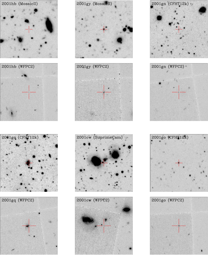
Only those candidates that were confirmed as SNe Ia were then scheduled for follow-up observations from the ground and with HST. In total, six SNe were sent for HST follow-up: one from the Subaru 2001 campaign and five from the Spring 2001 campaign. The SNe are listed in Tables 2 and 2.3. Finding charts are provided in Figure 1.
| Search | Instr./Tel. | Detector | Resolution | Observing dates |
|---|---|---|---|---|
| Spring 2001 | FORS1/Antu | Tektronix 2k2k CCD | 500 | 2001 April 21 – 22 |
| Spring 2001 | LRIS/Keck I | Tektronix 2k2k CCD | 850 | 2001 April 20 |
| Spring 2001 | ESI/Keck II | MIT-LL 2k4k CCD | 5000 | 2001 April 21 – 24 |
| Subaru 2001 | FOCAS/Subaru | SITe 2k4k CCD | 1000 | 2001 May 26 – 27 |
| MJD | Instrument and | Exp. | |||||
|---|---|---|---|---|---|---|---|
| IAU name | Search | (days) | telescope | (s) | |||
| SN 2001cw | Subaru 01 | 0.024 | 52056.6 | FOCAS/SubaruaaLong slit | 4200 | ||
| SN 2001gn | Spring 01 | 0.028 | 52023.1 | ESI/Keck IIbbEchellette | 9700 | ||
| SN 2001go | Spring 01 | 0.027 | 52021.3 | FORS1/AntuaaLong slit | 2400 | ||
| SN 2001gq | Spring 01 | 0.027 | 52020.3 | LRIS/KeckaaLong slit | 3600 | ||
| SN 2001gy | Spring 01 | 0.030 | 52021.3 | FORS1/AntuaaLong slit | 2400 | ||
| SN 2001hb | Spring 01 | 0.032 | 52024.3 | ESI/Keck IIbbEchellette | 3600 |
Here, we describe the analysis of data that were taken with ESI and LRIS. The analyses of the spectra taken with FORS1 and FOCAS (SN 2001cw, SN 2001go and SN 2001gy) are described in Lidman et al. (2005) and Morokuma et al. (2010) respectively. The spectra of these SN are shown in these papers and will not be repeated here.
2.1. ESI
The two highest redshift candidates, 2001gn and 2001hb, were observed with the echelette mode of ESI (Sheinis et al., 2002). A spectrum taken with the echellette mode of ESI and the slit covers the 0.39 µm to 1.09 µm wavelength range and is spread over 10 orders ranging in dispersion from 0.16 Å per pixel in the bluest order (order 15) to 0.30 Å per pixel in the reddest (order 6). The detector is a MIT-Lincoln Labs 2048 x 4096 CCD with 15 µm pixels. The slit width was set according to the seeing conditions and varied from to , which corresponds to a spectral resolution of . Compared to spectra obtained with low-resolution spectrographs, such as FORS1, FORS2, LRIS and FOCAS, the fraction of the ESI spectrum that is free of bright night sky lines from the Earth’s atmosphere is much greater. This allows one to de-weight the low signal-to-noise regions that overlap these bright lines when binning the spectra, a method that becomes inefficient with low-resolution spectra as too much of the spectra are de-weighted. Another advantage of ESI was that the MIT-LL CCD offered high quantum efficiency at red wavelengths and significantly reduced fringing compared to conventional backside-illuminated CCDs.
The data were reduced in a standard manner. The bias was removed by subtracting the median of the pixel values in the overscan regions, the relative gains of the two amplifiers were normalized by multiplying one of the outputs with a constant and the data were flat fielded with internal lamps. When extracting SN spectra, a bright star was used to define the trace along each order, and the spectrum of the SN was used to define the center of the aperture. Once extracted, the 10 orders were wavelength calibrated (using internal arc lamps and cross-checking the result with bright OH lines), flux calibrated and stitched together to form a continuous spectrum.
To reduce the impact that residuals from bright OH lines have on determining the redshift and classifying the candidate, the spectrum was weighted according to the inverse square of the error spectrum and then rebinned by a factor of 20, from 0.19 Å/pixel to 3.8 Å/pixel. The binning was chosen so that features from the host were not lost.
2.2. LRIS
The LRIS (Oke et al., 1995) data were taken with the 400/8500 grating and the GG495 order sorting filter and were reduced in a standard manner. The bias was removed with a bias frame, the pixel-to-pixel variations were normalized with flats that were taken with internal lamps and the background was subtracted by fitting a low order polynomial along detector columns. The fringes that were not removed by the flat were removed with a fringe map, which was the median of the sky subtracted data that was then smoothed with a 5x5 pixel box. The spectra were then combined, extracted, and calibrated in wavelength and flux.
The reduced spectrum of 2001gq is shown in Figure 18.
2.3. Spectral fitting and supernova typing
Light from the host and the SN are often strongly blended in the spectra of high redshift SN. To separate the two, we followed the spectral fitting technique described in Howell et al. (2005).
To classify the SNe, we used the classification scheme described in Lidman et al. (2005) and added to it the confidence index (CI) described in Howell et al. (2005). In the Lidman et al. (2005) scheme, an object is classified as a SN Ia if the Si II features at 4000 Å and/or 6150 Å or the S II W feature can be clearly identified in the spectrum or if the spectrum is best fit with the spectra of nearby SN Ia and other types do not provide a good fit. We qualify the classification with the keys “Si II” or “SF” in column 3 of Table 2.3 depending on whether the classification was done by identifying features or by using the fit. In the scheme described in Howell et al. (2005), these SNe would have a CI of 5 and 4, respectively.
Less secure candidates are classified as Ia*. The asterisk indicates some degree of uncertainty. Usually, this means that we can find an acceptable match with nearby SNe Ia; however, other types, such as SNe Ibc, also result in acceptable matches. These SNe have a confidence index of 3.
Redshifts based on the host have an accuracy that is better than 0.001, and are, therefore, quoted to three decimal places. Redshifts based on the fit are less accurate. For completeness, the redshifts and classifications reported in Lidman et al. (2005) and Morokuma et al. (2010) are also included.
The agreement between the phase, , of the best fit template and the corresponding phase, , obtained from the light curve fit is also shown in Table 2.3. The weighted average difference for all six spectra is days with a dispersion of 2.0 days. The dispersion is similar in magnitude to that found in other surveys (Hook et al., 2005; Foley et al., 2008).
| Spectroscopic | Template | |||||||
|---|---|---|---|---|---|---|---|---|
| IAU name | CI | classification | Redshift | match | (days) | (days) | (days) | |
| 2001cw | 3 | Ia* | SF | 1989B | -5 | +0.1 | ||
| 2001gn | 3 | Ia* | SF | 1990N | -7 | -3.6 | ||
| 2001go | 5 | Ia | Si II | 1992A | +5 | -1.5 | ||
| 2001gq | 3 | Ia* | SF | 1999bp | -2 | +3.1 | ||
| 2001gy | 5 | Ia | Si II | 1990N | -7 | -0.1 | ||
| 2001hb | 3 | Ia* | SF | 1989B | -7 | -0.2 | ||
3. Photometric observations
A total of nine different instruments, listed in Table 4, were used for the photometric follow-up of the SNe described in this work.
| Tel./Instr. | Scale | FOV | Detectors | Search |
|---|---|---|---|---|
| (′′/px) | (′) | |||
| CFHT/CFH12k | 0.206 | 4228 | 12 MIT 2k4k CCD | Spring 2001 |
| CTIO/MOSAIC II | 0.27 | 3636 | 8 SITe 2k2k CCD | Spring 2001 |
| VLT/FORS1 | 0.20 | 6.86.8 | 1 Tektronix 2k2k CCD | Spring 2001 |
| VLT/ISAAC | 0.1484 | 2.52.5 | Hawaii 1k1k HgCdTe array | Spring 2001 |
| NTT/SuSI2 | 0.08 | 5.55.5 | 2 EEV 2k4k CCD | Spring 2001 |
| Gemini/NIRI | 0.1171 | 2.02.0 | Aladdin 1k1k InSb array | Spring 2001 |
| HST/ACS | 0.05 | 2.42.4 | 2 SITe 2k4k CCD | Spring 2001 |
| HST/WFPC2 (PC) | 0.046 | 0.610.61 | 1 Loral Aerospace 800800 CCD | Both |
| Subaru/SuprimeCam | 0.20 | 3427 | 10 MIT/LL 2k4k CCD | Subaru 2001 |
All observations are listed in Table B. Here the Modified Julian Date (MJD) is the weighted average of all images taken during a given night except for the NIR data where data taken over several nights were combined. We do not report the MJD for combined reference images that were taken over several months.
3.1. Ground-based optical observations and reductions
We obtained ground-based optical follow-up data of the SNe through different combinations of passbands, shown in Figure 2, similar to Bessel and (Bessell, 1990), and SDSS (Fukugita et al., 1996). Here we used FORS1 (Appenzeller et al., 1998) at VLT and SuSI2 (D’Odorico et al., 1998) at NTT in addition to the search instruments. The SuSI2, MOSAIC II, CFH12k and SuprimeCam data were obtained in visitor mode, while the FORS1 observations were carried out in service mode.

All optical ground data were reduced (Raux, 2003) in a standard manner including bias subtraction, flat fielding and fringe map subtraction using the IRAF 222IRAF is distributed by the National Optical Astronomy Observatories, which are operated by the Association of Universities for Research in Astronomy, Inc., under the cooperative agreement with the National Science Foundation. software.
3.2. Ground-based IR observations and reduction
The two most distant SNe in the sample, 2001hb and 2001gn, were also observed from the ground in the near-IR. Both NIRI (Hodapp et al., 2003) and ISAAC (Moorwood et al., 1999) were used to observe 2001hb, while 2001gn was observed with ISAAC only.
The ISAAC observations were done with the Js filter and the NIRI observations were carried out with the filter. The transmission curves of the filters are similar to each other, and the transmission curve of the latter is shown in Figure 2. The red edges of the filters are defined by the filters and not by the broad telluric absorption band that lies between the and windows, and the central wavelength is slightly redder than the central wavelength of the filter of Persson et al. (1998). Compared to traditional band filters, photometry with the ISAACJs and NIRI band filters is less affected by water vapor and is therefore more stable.
The ISAAC observations were done in service mode and the data were taken on 14 separate nights, starting on 2001 May 7 and ending on 2003 May 30. Individual exposures lasted 30 to 40 s, and three to four of these were averaged to form a single image. Between images, the telescope was offset by to in a semi-random manner, and typically 20 to 25 images were taken in this way in a single observing block. The observing block was repeated several times until sufficient depth was reached.
The data, including the calibrations, were first processed to remove two electronic artifacts. In about 10% of the data, a difference in the relative level of odd and even columns can be seen. The relative difference is a function of the average count level and it evolves with time, so it cannot be removed with flat fields. In those cases where the effect is present, the data are processed with the eclipse333http://www.eso.org/projects/aot/eclipse/ odd-even routine. The second artifact, an electronic ghost, which is most easily seen when there are bright stars in the field of view, is removed with the eclipse ghost routine.
The NIRI observations were done in queue mode and the data were taken on 4 separate nights, starting on 2001 May 25 and ending 2002 Aug 5. Individual exposures lasted 60 s. Between images, the telescope was offset by to in a semi-random manner, and typically 60 images were taken in this way in a single observing sequence. The sequence was repeated several times until sufficient depth was reached.
Both the ISAAC and NIRI data were then reduced in a standard way with the IRAF XDIMSUM package and our own IRAF scripts. From each image, the zero-level offset was removed, a flatfield correction was applied, and an estimate of the sky from other images in the sequence was subtracted. Images were then combined with individual weights that depend on the median sky background and the image quality.
3.3. HST observations and reduction
Observing SN Ia at high- from space has an enormous advantage for accurately following their light curves. The absence of the atmosphere and the high spatial resolution allows high signal-to-noise measurements. The high spatial resolution also helps minimize host contamination through focusing the light over a smaller area. Space also permits observations at longer wavelengths where the limited atmospheric transmission and the high background degrade ground-based data.
High quality follow-up data were obtained for all six SNe using the Wide Field Planetary Camera 2 (WFPC2) on the Hubble Space Telescope (HST) during Cycle 9. All but two (2001cw and 2001gq) of the objects also have SN-free reference images taken during Cycle 10, with the Advanced Camera for Survey (ACS). WFPC2 consists of four 800x800 pixel chips of which one, the Planetary Camera (PC), has twice the resolution of the others. The SNe were always targeted with the lower left corner of the PC in order to place them closer to the readout amplifier so that the effects of charge-transfer inefficiency would be reduced. Images of the same target were obtained with roughly the same rotation for all epochs.
Each SN was followed in two bands. All SNe were observed in the F814W filter. Additionally, the F675W filter was used for the three SNe at and the F850LP filter was used for the high redshift targets. These filters were chosen to match the filters used on the ground and correspond approximately to rest frame UBV bands as illustrated in Figure 2.
The data were reduced with software provided by the Space Telescope Science Institute (STScI). WFPC2 images were processed through the STScI pipeline and then combined for each epoch to reject cosmic rays using the crrej task which is part of STSDAS 444The Space Telescope Science Data Analysis System (STSDAS) is a software package for reducing and analyzing astronomical data. It provides general-purpose tools for astronomical data analysis as well as routines specifically designed for HST data. IRAF package.
The ACS images were processed using the multi-drizzle (Fruchter & Hook, 2002) software, which also corrects for the severe geometric distortion of the instrument. For this we used the updated distortion coefficients from the ACS Data Handbook in November 2006, and drizzled the images to the resolution of the WFPC2 images . Note that the WFPC2 images were not corrected for geometric distortion at this stage.
4. Photometry of the ground-based data
The photometry technique applied to the optical ground-based data is the same as the one applied in Amanullah et al. (2008), except for the SuprimeCam band data. This is also very similar to the method (Fabbro, 2001) used in Astier et al. (2006), and is briefly summarized here:
-
1.
Each exposure of a given SN in a given passband was aligned to the best seeing photometric reference image.
-
2.
In order to properly compare images of different image quality we fitted convolution kernels, , modelled by a linear decomposition of Gaussian and polynomial basis functions (Alard & Lupton, 1998; Alard, 2000), between the photometric reference and each of the remaining images, , for the given passband. The kernels were fitted by using image patches centered on fiducial objects across the field.
-
3.
The background sky level for each image, , is not expected to have any spatial variation for a small patch, , centered on the SN with a radius of the worst seeing FWHM. We assume that the patch can be modelled by a point spread function (PSF) at the location of the SN, a model of the host galaxy and a constant offset for the sky,
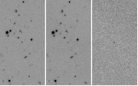
For a time-series of such patches we simultaneously fit the SN position, , and brightnesses, , host model, , and background sky levels, . We use a non-analytic host model with one parameter per pixel. This means that the model will be degenerate with the SN and the sky background. We break these degeneracies by fixing the SN flux to zero for all reference images and fix the sky level to zero in one of the images. Figure 3 shows an example of image patches, galaxy model residuals and resulting residuals when the full model has been subtracted, for increasing epochs.

Figure 3.— Ground-based -band images (patches) of 2001gq (three left columns; width ) and 2001go (three right columns; width ). Each triplet represents from left to right the fully reduced data, the galaxy model subtracted data, and a profile plot where the full galaxy + PSF model has been subtracted from the data. The profile plot shows the deviation from zero in standard deviations of the noise versus the distance from the SN position in pixels. Epoch increases from top to bottom. The images in the last row are the reference image, obtained approximately one year after discovery. The different image sizes (patches) reflect differences in image quality. A small image represents good seeing conditions.
The SN light curves were obtained in this manner for one filter and instrument at a time where SN-free reference images were available. In the cases where SN-free references did not exist for a given telescope, reference images obtained with other telescopes were used instead.
For the IR image of 2001hb, we performed aperture photometry directly on the images, assuming the SN to be hostless for the purpose of band photometry, since no host could be detected at the limit of the ACS references (see below). For the IR image of 2001gn, we carried out steps 1–2 above, and then subtracted the reference image (Figure 4) and did aperture photometry on the resulting image. In both cases the SN positions from the HST images were used for centroiding the aperture and the diameter was chosen to maximize the signal-to-noise ratio. The fluxes are corrected to larger apertures by analyzing bright stars in the same image.
The band data for 2001cw was analyzed together with a larger sample of SNe discovered at Subaru. The details of this analysis are given in Yasuda et al. (in preparation).
4.1. Calibration of the ground-based data
Nightly observations of standard stars were not available for all optical instruments and filters. Instead the recipe from Amanullah et al. (2008), using SDSS (Adelman-McCarthy et al., 2007) measurements of the field stars was applied. However, the SDSS filter system (Fukugita et al., 1996) differs significantly from the filters used in this search except for the SuprimeCam band. To overcome this difference, we fitted relations between the SDSS filter system and the Landolt system (Landolt, 1992) in a similar manner to Lupton (2005), using stars with SDSS and Stetson photometry (Stetson, 2000). Stetson has been publishing photometry of a growing list of faint stars that is tied to the Landolt system within mag (Stetson, 2000). The most up to date version can be obtained from the Canadian Astronomy Data Center555 http://www.cadc.hia.nrc.gc.ca/community/STETSON/archive/ . In contrast to Lupton (2005), we applied magnitude, uncertainty and color cuts (, mag in and and ) for the stars that went into the fit. We also applied a outlier cut after our initial fit (and lost about of the sample). After refitting, the following relations were derived for the Landolt and filters
which are also shown in Figure 5. The results for are close to the ones derived by Lupton (2005) as well as to Tonry et al. (2003) who performed a similar operation. Neither Tonry et al. (2003) nor Lupton (2005) present fits for vs .

By forcing , we determined that there is a scatter of mag coming from intrinsic spectral distributions. This is a systematic uncertainty for individual stars, but will average out when a big sample is used, assuming that the color distribution of the sample is similar to the stars used to derive the relations.
The transformations were applied to the SDSS stellar photometry of our SN field, and these were then used as tertiary standard stars in order to tie the SN photometry to the Landolt system. The flux of the stars was determined on the photometric reference for each light curve build using the same method as for the SN and with the same PSF model that was used for fitting the SN fluxes. A zero-point relation of the form
| (1) |
could then be fitted between the measured stellar fluxes, , and their Landolt magnitudes, . Here is the zero point and is the color term for the filter. We applied the same color cuts () to the stars that went into the fit.
Unfortunately we did not have enough stars over a wide enough color range to accurately fit the color term. Instead, we used values from the literature or from the observatories, which are summarized in Table 4.1. The zero-points could then be derived from equation (1). The values obtained this way are the sums of three components; the instrumental zero-point, the aperture correction to the PSF normalization radius and the atmospheric extinction for the given airmass, and are shown along with the SN fluxes in Table B.
We also calculated color terms synthetically by using Landolt standard stars that have extensive spectrophotometry from Stritzinger et al. (2005). The synthetic Vega magnitudes of the stars were calculated by multiplying the spectra and the Vega spectrum (Bohlin, 2007) with the filter and instrument throughputs provided by the different observatories. The color terms were then fitted by assuming a linear relation for the deviation between the synthetic and the Landolt magnitudes as a function of the Landolt color. The resulting fitted synthetic terms are also presented in Table 4.1.
The difference is mag for all but the CFH12k -band, where there is a significant discrepancy. A mismatch between the effective filter transmission curves we use and the true photometric system is most likely the origin of this. We have investigated if the deviation could be explained by the differences in quantum efficiencies between the different chips of the detector which are presented on the CFH12k webpage. However these differences propagated to the color term results in relatively low scatter and deviates significantly from the measured value.
For the purpose of fitting the zero-points, we can use the measured color terms, but for light curve fitting erroneous filter transmissions could introduce systematic effects. In order to study the potential impact on the light curve fits we modified the filters to match the measured color terms. The modifications were implemented by either shifting or clipping the filters until the synthetic color terms matched all measured values for a given filter (e.g. or vs , and for the ELIXIR measurements for the -band). The light curves were then refitted using the modified filter transmissions and the resulting values were compared. Since the light curves are tightly constrained by the high precision HST data, the modified filter only leads to negligible differences (less than of the statistical uncertainty) in the fitted parameters.
The -band data, on the other hand, were calibrated using G-type standard stars from the Persson LCO standard star catalogue (Persson et al., 1998). Since the ISAAC and NIRI -band filters are slightly redder and narrower than the Persson -band filter, we subtracted magnitudes from the ISAAC and NIRI zero points to place the ISAAC and NIRI IR photometry onto the natural system. Since the data were taken over many nights, the photometry was carefully cross checked. Differences in the absolute photometry usually amount to less than magnitudes, which we conservatively adopt as our zero-point uncertainty.
5. Photometry of the HST data
A modified version of the photometric technique from Knop et al. (2003) was used for the HST data presented here. This is similar to the method used for the ground-based optical data above, but instead of aligning and resampling all images to a common frame, the hostSN model is resampled to each individual image. A procedure like this is preferred when the PSF FWHM is of the same order as the pixel scale, and it also preserves the image noise properties.
Linear geometric transformations were first fitted from each image, , in a given filter to the deepest image of the field using field objects. Due to the similar orientation of the WFPC2 images, linear transformations were sufficient for these, and the geometric distortion of WFPC2 could be ignored. This was however not the case for the transformations between the ACS and WFPC2 images and the distortion was then hardcoded into the fitting procedure. Due to the sparse number of objects in the tiny PC field the accuracy of all transformations were only good to pixel ( FWHM). Unfortunately, using objects from the remaining three chips for the alignment did not lead to improved accuracy, which is probably due to small movements of the chips between exposures (Anderson & King, 2003). This alignment precision was not enough for PSF photometry, and we therefore allowed the SN position, to float for the individual images which increased the alignment precision by a factor of 10. Allowing this extra degree of freedom could bias the results toward higher fluxes since the fit will favor positive noise fluctuations. However, as in Knop et al. (2003), this was shown to be of minor importance by studying the covariance between the fitted flux and SN position.
The full model used to describe each image patch can be expressed as
| (2) |
Here is the value in pixel on image , is the SN flux, the point spread function, the host galaxy model that is parameterized by and the local sky background. The fits were carried out using a minimization approach using MINUIT (James & Roos, 1975).
Four SNe in the sample had ACS reference images, and for these cases we used field objects to fit non-analytic convolution kernels, , between the PC chip and the drizzled ACS image. These accounted for the difference in quantum efficiency and PSF shape between the two instruments. When kernels were used, the uncertainties of individual pixels were propagated and the correlation between pixels produced by the convolution were taken into account. Also, in this case equation (2) above was modified so with both the PC images and the PC PSF being convolved with the fitted kernel.
The PSF, , of the WFPC2 PC chip was simulated for each filter and pixel position using the Tiny Tim software (Krist, 2001) and normalized to the WFPC2 calibration radius . We also did an extensive test where we iteratively updated the simulated PSF based on the knowledge of the SN epoch, and therefore the approximate spectral energy distribution (SED), but this did not have any significant effect on the fitted fluxes. The Tiny Tim PSF was generated to be subsampled by a factor of 10. For each iteration in the fitting procedure, any shift of the PSF position was first applied in the subsampled space. The PSF was then re-binned to normal sampling and convolved with a charge diffusion kernel (Krist, 2001) before it was added to the patch model.
For three of the SNe, 2001cw, 2001gq and 2001hb we used an analytical model for the host galaxy. Both 2001cw and 2001gq are offset from the core of their respective host galaxies and we therefore chose not to obtain SN-free references images for these. Instead the hosts could be modeled by a second order polynomial and constrained by the galaxy light in the vicinity of the SNe. For 2001hb, we did obtain a deep ACS reference image but no host could be detected. For this SN we used a simple plane to model the host which was further constrained by fixing the SN flux to zero for the ACS reference. One caveat with analytical host modelling in general is that the patch size must be chosen with care. The model will only work if there is no dramatic change in the background across the patch, which is an assumption that is likely to fail if the patch is too large and includes the host galaxy core. On the other hand the patch can not be too small either in order to successfully break the degeneracy between the SN and the background.
To make sure that the choice of host model does not bias the fitted SN fluxes we required, in addition to clean residuals once the SN + host was subtracted from the data, that the fitted SN fluxes were insensitive to variations in the patch size of a few pixels. Further, for 2001gq, we tested the host model by putting fake SNe at different positions around the core of the host. The distances to the core and the fluxes of the fakes were always chosen to match the corresponding values for the real SN, and the retrieved photometry was always within the expected statistical uncertainty.
The recipe described above could not be used for the remaining three SNe in the sample, since they were located too close to the cores of their host galaxies. Additionally, the hosts have small angular sizes and the light gradients in the vicinity of the SNe were steep enough to lead to biased photometry due to the coarse geometric alignment. To overcome this we changed the photometric procedure slightly. Instead of fitting the SN position on each image, we chose to fit it only on the geometric reference image, and then introduce a free shift for the whole model. That is, in this case we used the galaxy model SN for the patch alignment. However, this procedure did force us to apply some constraints on the galaxy modelling. Using a non-analytic pixel model, the approach used for the ground-based optical data, was not feasible. It slowed down the fits considerably and rarely converged. Instead we chose to use the ACS images of the host galaxies directly. The ACS references were much deeper then the WFPC2 data and choosing this procedure did not increase the uncertainty of the fitted fluxes.
A general problem with doing photometry on HST images is that CCD photometry of faint objects over a low background suffers from an imperfect charge transfer, which will lead to an underestimate of the flux. We used the Charge Transfer Efficiency (CTE) recipe for point sources from Dolphin (2009). The correction for our data is usually around – but it can be as large as . The uncertainties of the corrections were propagated to the flux uncertainties. The corrected SN fluxes are given in Table B together with the instrumental zero-points, which were also obtained from Andrew Dolphin’s webpage
6. Light curve fitting
SN Ia that have bluer colors or broader light curves tend to be intrinsically brighter (Phillips, 1993; Tripp, 1998). Several methods of combining this information into an accurate measure of the relative distance have been used (Riess et al., 1996; Goldhaber et al., 2001; Wang et al., 2003; Guy et al., 2005, 2007; Jha et al., 2007; Conley et al., 2008).
K08 consistently fitted all light curves using the SALT (Guy et al., 2005) fitter, which is built on the SN Ia SED from Nugent et al. (2002). In this paper, we use SALT2 (Guy et al., 2007), which is based on more data.
Conley et al. (2008) compared the performances of different light curve fitters while also introducing their own empirical fitter, SiFTO, and concluded that SALT2 along with SiFTO perform better than both SALT (which is conceptually different from its successor SALT2) and MLCS2k2 (Jha et al., 2007) when judged by the scatter around the best-fit luminosity distance relationship. Furthermore, SALT2 and SiFTO produce consistent cosmological results when both are trained on the same data. Recently KS09 made a thorough comparison between SALT2 and their modified version of MLCS2k2 (Jha et al., 2007) for a compilation of public data sets, including the one from the SDSS SN survey. The two light curve fitters result in an estimate of (for a flat CDM cosmology) that differs by . The difference exceeds their statistical and systematic (from other sources) error budgets. They determine that this deviation originates almost exclusively from the difference between the two fitters in the rest-frame -band region, and the color prior used in MLCS2k2. They also noted that MLCS2k2 is less accurate at predicting the rest-frame -band using data from filters at longer wavelengths.
This difference in -band performance is not surprising: observations carried out in the observer-frame -band are in general associated with a high level of uncertainty due to atmospheric variations. While the training of MLCS2k2 is exclusively based on observations of nearby SNe, the SiFTO and SALT2 training address this difficulty by also including high redshift data where the rest-frame -band is observed at redder wavelengths. This approach also allows these fitters to extend blueward of the rest-frame -band.
In addition, for this paper, we have conducted our own test validating the performance of SALT2 by carrying out the Monte-Carlo simulation described in 7.3.6, where we compare the fitted SALT2 parameters to the corresponding real values for mock samples with poor cadence and low signal-to-noise drawn from individual well-measured nearby SNe.
Given these tests that have been carried out on SALT2, and its high redshift source for rest-frame -band, we have chosen to use SALT2 in this paper.
6.1. SALT2
The SALT2 SED model has been derived through a pseudo-Principal component analysis based on both photometric and spectroscopic data. Most of these data come from nearby SN Ia data, but SNLS supernovae are also included. To summarize, the SALT2 SED, , is a function of both wavelength, , and time since -band maximum, . It consists of three components; a model of the time dependent average SN Ia SED, , a model of the variation from the average, , and a wavelength dependent function that warps the model, . The three components have been determined from the training process (Guy et al., 2007) and are combined as
where , and are free parameters that are fit for each individual SN.
Here, , describes the overall SED normalization, , the deviation from the average decline rate () of a SN Ia, and , the deviation from the mean SN Ia color at the time of -band maximum. These parameters are determined for each observed SN by fitting the model to the available data. The fit is carried out in the observer frame by redshifting the model, correcting for Milky Way extinction (using the CCM-law from Cardelli et al. (1989) with ), and multiplying by the effective filter transmission functions provided by the different observatories. All synthetic photometry is carried out in the Vega system using the spectrum from Bohlin (2007). Following Astier et al. (2006) we adopt the magnitudes mag (Fukugita et al., 1996) for Vega. For the near-infrared we adopt the values and .
In the fit to our data, we take into account the correlations introduced between different light curve points from using the same host galaxy model. We also chose to run SALT2 in the mode where the diagonal of the covariance matrix is updated iteratively in order to take model and -correction uncertainties into account. See Guy et al. (2007) for details on this. The Milky Way reddening for our supernovae from the Schlegel et al. (1998) dust maps is given in Table 2. The results of the fits are shown in Table 6.1 and plotted in Figure 6 together with the data.

The three parameters
can for each SN be combined to form the distance modulus (Guy et al., 2007),
| (3) |
where is the absolute -band magnitude. The resulting color and light curve shape corrected peak -band magnitudes, , are presented in the third column of Table 6.1. The parameters , and are nuisance parameters which are fitted simultaneously with the cosmological parameters.
7. The Union2 Compilation
K08 presented an analysis framework for combining different SN Ia data sets in a consistent manner. Since then two other groups (H09 and KS09) have made similar compilations, using different fitters. In this work we carry out an improved analysis, using and refining the approach of K08. We extend the sample with the six SNe presented here, the SNe from Amanullah et al. (2008), the low- and intermediate- data from Hicken et al. (2009a) and Holtzman et al. (2008) respectively666The SALT2 fit results for these samples are presented along with the entire Union2 compilation fits at http://supernova.lbl.gov/Union/..
First, all light curves are fitted using a single light curve fitter (the SALT2 method) in order to eliminate differences that arise from using different fitters. For all SNe going into the analysis we require:
-
1.
data from at least two bands with rest-frame central wavelengths between Å and Å, the default wavelength range of SALT2
-
2.
that there is at least one point between days and rest frame days relative to the -band maximum.
-
3.
that there are in total at least five valid data points available.
-
4.
that the fitted values, including the fitted uncertainties, lie between . This is a more conservative cut than that used in K08 and results in several poorly measured SNe being excluded. Part of the discrepancy observed by KS09 when using different light curve models could be traced to poorly measured SNe.
-
5.
that the CMB-centric redshift is greater than .
We also exclude one SN from the Union compilation that is 1991bg-like, which neither the SALT nor the SALT2 models are trained to handle. Note that another 1991bg-like SN from the Union compilation was removed by the outlier rejection. All SNe Ia considered in this compilation are listed in Table B. For each SN, the redshift and fitted light curve parameters are presented as well as the failed cuts, if any.
It should be pointed out that the choice of light curve model also has an impact on the sample size. Using SALT2 will allow more SNe to pass the cuts above, since the SALT2 model covers a broader wavelength range than SALT. This is particularly important for high- data that heavily rely on rest-frame data. For example, two net SNe would have been cut from the Riess et al. (2007) sample with the SALT model.
7.1. Revised HST zero-points and filter curves
Since Riess et al. (2007), the reported zero-points of both NICMOS and ACS were revised. For the F110W and F160W filters of NICMOS, the revision is substantial. Using the latest calibration (Thatte et al., 2009, and references within), the revised zero-points are, for both filters, approximately fainter than those reported in Riess et al. (2007) and subsequently used by K08.
For SNe Ia at , observations with NICMOS cover the rest frame optical, so the fitted peak -band magnitudes and colors and the corrected -band magnitudes of these SNe Ia depend directly on the accuracy of the NICMOS photometry. With the new zero-points, SNe Ia at are measured to be fainter and bluer. Our current analysis also corrects an error in the NICMOS filter curves that were used in K08, which also acts in the same direction.
In the introduction, we had noted that almost all SNe at were redder than the average SN color over the redshift interval to . This is surprising as redder SNe are also fainter and should therefore be the harder to detect in magnitude limited surveys. K08 noted that these SNe, after light curve shape and color corrections, are also on average mag brighter than the line tracing the best fit CDM cosmology. They also noted that this was the reason for the relatively high value for the binned value of in the redshift bin.
After taking the NICMOS zero-point and filter updates just discussed into account, we repeated the original K08 analysis. This made the NICMOS observed SNe up to mag fainter, and there no longer is a significant offset from the best fit cosmology. Nor are these SNe unusually red when compared to SNe over the redshift interval to . For SALT2 the SNe at have an average color of , compared to for , and no significant offset in the Hubble diagram.
There could however still be unresolved NICMOS issues. For example the NICMOS SN photometry depends on extrapolating the non-linearity correction to low flux levels. We have a program (HST GO-11799) to obtain a calibration of NICMOS at low flux levels. The photometry of the SNe observed with NICMOS will be revised once this program is completed. The new data presented in this paper also allow us another route to check this color discrepancy with IR data independent of the NICMOS calibration.
7.2. Fitting Cosmology
Following Conley et al. (2006) and K08, we adopt a blind analysis approach for cosmology fitting where the true fitted values are not revealed until the complete analysis framework has been settled. The blind technique is implemented by adjusting the magnitudes of the SNe until they match a fiducial cosmology (, ). This procedure leaves the residuals only slightly changed, so that the performance of the analysis framework can be studied. The best fitted cosmology with statistical errors is obtained through an iterative -minimization of
| (4) |
where,
| (5) |
is the propagated error from the covariance matrix, , of the light curve fits, with and being the and color correction coefficients of equation (3). Uncertainties due to host galaxy peculiar velocities of km/s and uncertainties from Galactic extinction corrections and gravitational lensing as described in 7.3 are included in . A floating dispersion term, , which contains potential sample-dependent systematic errors that have not been accounted for and the observed intrinsic SN Ia dispersion, is also added. The value of is obtained by setting the reduced to unity for each sample. Computing a separate for each sample prevents samples with poorer-quality data from increasing the errors of the whole sample. This approach does however still assume that all SNe within a sample are measured with roughly the same accuracy. If this is not the case there is a risk in degrading the constraints from the sample by down weighting the best measured SNe. It should also be pointed out that the fitted values of will be less certain for small samples and can therefore deviate significantly from the average established by the larger samples (in particular, the six high- SNe presented in this work are consistent with ), as are three other samples.
A number of systematic errors are also being considered for the full cosmology analysis. These are taken into account by constructing a covariance matrix for the entire sample which will be described below in 7.3. The terms in the denominator of equation (4) are then added along the diagonal of this covariance matrix.
Following K08, we carry out an iterative minimization with outlier rejection. Each sample is fit for its own absolute magnitude by minimizing the sum of the absolute residuals from its Hubble line (rather than the sum of the squared residuals). The line is then used for outlier rejection. This approach was investigated in detail in K08, and it was shown with simulations that the technique is robust and that the results are unaltered from the Gaussian case in the absence of contamination and that in the presence of a contaminating contribution, its impact is reduced. Table 7.2 summarizes the effect of the outlier cut on each sample. We also note that the residuals have a similar distribution to a Gaussian in that of the sample is outside of .
Figure 7 shows the individual residuals and pulls from the best fit cosmology together with the fitted SALT2 colors for the different samples. The photometric quality is illustrated by the last column in the figure showing the color uncertainty. It is notable how the photometric quality on the high redshift end has improved from the K08 analysis. This is due to the extended rest-frame range of the SALT2 model compared to SALT.

Figure 8 shows the diagnostics used for studying the consistency between the different samples. The left panel shows the fitted values for each sample together with the RMS around the best fitted cosmology. The intrinsic dispersion associated with all SNe can be determined as the median of as long as the majority of the samples are not dominated by observer-dependent uncertainties that have not been accounted for. The median for this analysis is mag, indicated by the leftmost dashed vertical line in the figure. The two mid-panels show the tensions for the individual samples, by comparing the average residuals from the best-fit cosmology. The two panels show the tensions without and with systematic errors (described in 7.3) being considered. Most samples fall within and no sample exceeds . The right panel shows the tension of the slopes of the residuals as a function of redshift. This test may not be very meaningful for sparsely sampled data sets, but could reveal possible Malmquist bias for large data sets.
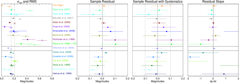
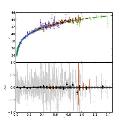
The SNe introduced in this work show no significant tension in any of the panels. The Hubble residuals for these are also presented in Figure 9. Here, the individual SNe are consistent with the best fit cosmology.
All tables and figures, including the complete covariance matrix for the sample, are available in electronic format on the Union webpage777http://supernova.lbl.gov/Union/. We also provide a CosmoMC module for including this supernova compilation with other datasets.
7.3. Systematic errors
The K08 analysis split systematic errors into two categories: the first type affects each SN sample independently, the second type affects SNe at similar redshifts. Malmquist bias and uncertainty in the colors of Vega are examples of the first and second type, respectively. Typical numbers were derived for both of these types of systematics, and they were included as covariances888Note that adding a covariance is equivalent to minimizing over a nuisance parameter that has a Gaussian prior around zero; the discussion in K08 is in terms of these nuisance parameters. This is further discussed in Appendix C. between SNe. Each sample received a common covariance, and all of the high-redshift () SNe shared an additional common covariance.
Other analyses (Astier et al. (2006), Wood-Vasey et al. (2007), KS09) have estimated the effect on for each systematic error and summed these in quadrature. However, Kim & Miquel (2006) show that parameterizing systematic errors (such as uncertain zeropoints) with nuisance parameters is a more apropriate approach and gives better cosmological constraints. For this analysis, all contributing factors, described below, were translated to nuisance parameters, which were then incorporated into a covariance matrix for the distances of the individual SNe. Appendix C contains the details of converting nuisance parameters to a covariance matrix.
7.3.1 Zero-point Uncertainties
In order to correctly propagate calibration uncertainties, we computed numerically the effect of each photometric passband on the distance modulus. For each SN, the photometry from each band was shifted in turn by magnitudes and then refit for . We then computed the change in distance modulus, giving for each band. A list of zero-point uncertainties is given in Table 8. For two SNe, and , with calibrated photometry obtained in the same photometric system, the zero-point uncertainty, of that system was propagated into the covariance matrix element as according to Appendix C.2.
This procedure is a more efficient way of including zero-point uncertainties than including a common magnitude covariance (multiplicative in flux space) when performing all of the light curve fits. In testing, both of these methods gave results that agreed at the couple of a percent level. Our method has the advantage that the zero-point errors can be adjusted without rerunning the light curve fits.
Zero-point uncertainties are one of the largest systematic errors (see Table 9). However, we should note that this number is based on a heterogeneous assessment of errors from different datasets (Table 8); the accuracy will vary.
| Source | Band | Reference | |
|---|---|---|---|
| HST | WFPC2 | 0.02 | Heyer et al. (2004) |
| ACS | 0.03 | Bohlin (2007) | |
| NICMOS | 0.03 | Thatte et al. (2009) | |
| SNLS | , , | 0.01 | Astier et al. (2006) |
| 0.03 | |||
| ESSENCE | , | 0.014 | Wood-Vasey et al. (2007) |
| SDSS | 0.014 | Kessler et al. (2009) | |
| , , | 0.009 | ||
| 0.010 | |||
| This paper | , | 0.03 | |
| 0.02 | |||
| Other | -band | 0.04 | Hicken et al. (2009a) |
| Other Band | 0.02 | Hicken et al. (2009a) |
7.3.2 Vega
Astier et al. (2006) estimated the broadband Vega magnitude system uncertainty to be within by comparing spectroscopy from D. S. Hayes, L. E. Pasinetti, & A. G. D. Philip (1985) and Bohlin & Gilliland (2004). In their analysis, only the uncertainties of Vega colors had implications for cosmological measurements, which they chose to include by adopting a flux uncertainty linear in wavelength that would offset the Vega color by 0.01. The uncertainty of Vega is the single largest source of systematic error when estimating , as shown in Table 9, suggesting that a better-understood reference would allow for a significant reduction in systematic errors.
KS09, and recently SNLS (Regnault et al., 2009), chose BD as their primary reference star. This star has the advantage of having a well-known SED, measured Landolt magnitudes (in contrast to Vega) and colors that are close to the average colors of the Landolt standards (in contrast to Vega which is much bluer). KS09 studied the implications of switching between BD and Vega and found zeropoints consistent to .
Given this small difference between using BD and Vega, we have chosen, for this work, to continue using Vega as our primary reference star. To account for the uncertainty of the magnitude of Vega on the Landolt system, we have assumed a correlated uncertainty of mag for all photometry with a rest-frame wavelength in each of six wavelength intervals defined by the following wavelength boundaries: 2900Å, 4000Å, 5000Å, 6000Å, 7000Å, 10000Å, 16000Å.
7.3.3 Rest-frame -Band
SNe Ia are known to show increasing spectroscopic and photometric diversity for wavelengths shorter than the rest-frame -band. Part of this could perhaps be explained by differences in progenitor metallicity (Hoeflich et al., 1998; Lentz et al., 2000), but the spectral variations in the rest-frame UV (Ellis et al., 2008) are larger than predicted by existing models.
As discussed in Section 6, KS09 studied how well the SALT2 model describes the rest-frame -band by first running SALT2 with the rest frame -band excluded. Using these fits, they then generated a model for the rest frame -band and binned the magnitude residuals from the actual rest-frame -band data as a function of phase. For the SDSS and SNLS datasets, the residuals around the time of maximum are . For SNLS, this is not surprising, as the SNLS data was used to train the SALT2 model. In this analysis, we use the SDSS sample as a validation set, and include a correlated magnitude uncertainty for all photometric bands bluer than rest-frame 3500Å.
We note that the HST and low-redshift datasets are less useful for assessing the size of rest-frame -band uncertainty. For the HST data, the light curves are poorly constrained without the rest-frame -band. In the case of the nearby sample, the rest-frame -band overlaps with the observed -band for which accurate photometry is generally difficult to obtain (any potential problems with the nearby -band will not impact the light curve fits much, as the low- fits are typically very well constrained with the remaining bands).
7.3.4 Malmquist bias
K08 added a magnitude covariance for each sample representing Malmquist bias uncertainty. More recently, KS09 completed a thorough simulation of selection effects for each of the samples in their analyses. They find a 0.024 change in when making a correction for selection effects. As the magnitude covariance yields a quite similar 0.026 error on , and conducting a full simulation is beyond the scope of this work, we reuse the covariance from K08.
7.3.5 Gravitational lensing
The effects from gravitational lensing on the Hubble diagram have been discussed in detail in the literature (Sasaki, 1987; Linder, 1988; Bergström et al., 2000; Amanullah et al., 2003; Holz & Linder, 2005). Gravitational lensing only affects the high redshift end of the data that is currently available, and potential bias on the cosmological parameters from the analysis carried out here due to the asymmetry of the lensing probability density function is expected to be negligible. We adopt the K08 approach of only treating gravitational lensing as a statistical uncertainty by adding a value of (Holz & Linder, 2005) in quadrature to in equation (4). This is a conservative approach with respect to the values presented by Jönsson et al. (2006), where they attempt to measure the lensing of individual SNe by determining the mass distribution along the line of sight. A very important conclusion of their work is that there is no evidence for selection effects due to lensing of the high-redshift SNe.
7.3.6 Light curve model
We have studied any potential bias that could arise from poor light curve sampling, by carrying out a similar analysis to K08, updated for SALT2. We use nine BVR AQUAA templates (Strovink, 2007) constructed from observations of very well-observed nearby supernovae. Each set of BVR templates is combined with a SALT2 -band template generated for that supernova, as there were insufficient observations in the -band to construct an AQUAA template.
Mock data sets are then sampled from these templates with the same rest frame dates and signal-to-noise ratios of the real SNe in our sample. The mock sets are then fitted with SALT2 and the offset between AQUAA corrected magnitude and the corresponding SALT2 fitted value is investigated as a function of the fitted phase of each supernova’s first data point (the phase is with respect to -band maximum). K08 looked at other possible biases, but first phase was the only significant one found. The test is carried out for each of the nine template SNe.
For SNe with a first phase at -band maximum, the average bias is close to zero, with an RMS of about 0.03. For SNe with a first phase at six days past -band maximum, the average bias is still close to zero, but the RMS has increased to about 0.08. Of course, our nine SN templates might not be a representative sample, but these results are encouraging, since they both suggest that there is no significant bias and indirectly validate the SALT2 performance with respect to the AQUAA templates.
We use a first phase cut of six days, but we conservatively give each SN that has first phase greater than zero a magnitude covariance. Note that SALT2 does not stretch its definition of phase with light curve width.
7.3.7 Contamination
As already mentioned, we perform an iterative minimization with a outlier rejection before fitting cosmology. In K08 we showed that this technique greatly reduces the impact of potential contamination, while maintaining roughly Gaussian statistics. We carried out a Monte-Carlo study showing that the effect of contamination on any individual sample is limited to less than magnitudes. This is under the assumption that the dispersion of the contaminating distribution is of the same order, or greater than, the dispersion of SNe Ia and that the contamination is less than . We include a magnitude uncertainty, correlated for each sample, to account for possible contamination.
7.3.8 Minimum redshift
In order to test for possible effects from using a given minimum redshift cut, we started by constructing a new sample with no minimum redshift. Using this sample, we performed fits which allowed the absolute magnitude to vary independently below and above a dividing redshift in the range to . This procedure should test for a Hubble bubble or significantly correlated peculiar velocities. The extra degree of freedom allowed by this step in improved the by regardless of the dividing redshift and the inclusion of systematic errors. This confirms the results of Conley et al. (2007) for SALT2. We conclude that there is no statistically significant difference between minimum redshifts and use the value of 0.015, as was used in the K08 analysis.
7.3.9 Galactic extinction
All light curve photometry is corrected for Galactic extinction using the extinction law from Cardelli et al. (1989), assuming , together with the dust maps from Schlegel et al. (1998).
In the same procedure as with calibration uncertainties, we increased the Galactic by 0.01 for each supernova and repeated the fit, giving . A statistical and systematic error was assumed for the Galactic extinction of each supernova (Schlegel et al., 1998).
7.3.10 Intergalactic extinction
Dimming of SNe Ia by hypothetical intergalactic gray dust has been suggested by Aguirre (1999) as an alternative to dark energy to explain the SN results (Goobar et al., 2002). This potential dimming was however constrained by studying the colors of high- quasars (Mörtsell & Goobar, 2003; Östman & Mörtsell, 2005) and by observations SNe Ia in the rest frame I-band (Nobili et al., 2005, 2009).
Another possible extinction systematic comes from the dust in galaxy halos that are along the line of sight. Ménard et al. (2009b) used distant quasars to detect and measure extinction in galactic halos at . They find an average for their galaxies of . Using their observed , we find an average rest frame -band extinction of magnitudes per intersected halo, assuming . At redshift 0.5, an average of three halos have been intercepted. At redshift 1.0, the average is seven.
There are three mitigating factors. One is that expansion redshifts photons between the supernova and the intervening galaxy. The CCM law decreases with wavelength (in the relevant wavelength range), so less light is absorbed. Ménard et al. (2008) finds that , which we use to scale the extinction. Finally, most of the extinction is corrected by color correction. The exact amount corrected depends on the redshift and the filters used in the observations, but is around two thirds.
We find an error on of 0.008 due to this extinction, significantly lower than the value of 0.024 derived by Ménard et al. (2009a). However, they used , rather than ; the fraction of extinction that is corrected by the color correction will decrease with . We also numerically sum the CCM laws, rather than using an analytic approximation. Since we know the exact redshift and filters used in each observation, we can exactly calculate the amount of extinction already handled by the color correction (using our values), without approximation.
7.3.11 Shape and Color Correction
The most uncertain contribution to the dimming of SNe Ia is host galaxy extinction. Several studies of SN Ia colors (Guy et al., 2005, 2007; Wang et al., 2008; Nobili & Goobar, 2008, and references therein) indicate that the observed SN Ia reddening does not match the Galactic CCM extinction law with . A stronger wavelength dependence has been found in the optical in most cases, and it remains unclear if CCM models with any value of can be used to describe the data accurately. It is possible that the observed steep reddening originates from a mixture of local effects and host galaxy extinction. Local effects could be intrinsic SN variations, but also multiple scattering on dust in the circumstellar environment has been suggested (Wang, 2005; Goobar, 2008). This model is potentially supported by detection (Patat et al., 2007; Simon et al., 2009; Blondin et al., 2009) of circumstellar material but also by color excess measurements for two of the best observed reddened SN Ia (Folatelli et al., 2010) being consistent with the expected extinction from circumstellar material.
The SALT2 method approaches the lack of a consistent understanding of SN Ia reddening by adopting a purely empirical approach. For SALT2, the SN Ia luminosity is standardized by assuming that the standardization is linear in both and as described in equation (3), where is the empirically determined correction coeffecient that accounts for all linear relations between color and observed peak magnitude. For example if the only source for such SN Ia reddening originated from CCM extinction then is identically equal to . We test this approach and propagate relevant systematic uncertainties by dividing the full sample into smaller sets and carrying out independent fits for the and correction coefficients, and , as shown in Table 8.3.
When subdividing into redshift bins, we find that the values of and for the full sample are consistent with values for the three first redshift bins. It is encouraging to see consistency between the global values fit for the full dataset and the values in the best-understood redshift range. Beyond this important test, we also note that the value of in the redshift range 0.5 to 1 is significantly lower than the other values, while the value for is higher than the global value, but is poorly measured. The trend is similar to what was seen in KS09, but we use different binning. This behavior is inconsistent with a monotonic drift in redshift, so we consider other explanations for these results. That conclusion is also supported by the observation that samples at similar redshifts (e.g. Miknaitis et al. (2007) and Astier et al. (2006)) can have very different values of when fitted independently. The value of is consistent across redshift ranges, except at , where many light curves are so poorly sampled that it may not be possible to assign reasonable errors.
When subdividing into the four largest data sources (the lower half of Table 8.3), we find values of and generally consistent with the global values, with the exception of a lower value of for the SNLS SNe (Astier et al., 2006). In general, ignoring or underestimating the errors in or will decrease the associated correction coefficients, and , as investigated in K08 and KS09 and this may be relevant here. Specifically, two potential sources of problems are an incomplete understanding of calibration and underestimated SN model variations, either of which could affect these fits. If the SNLS SNe are physically different, and they are allowed their own , then shifts by 0.02. Alternatively, as one is used for the global sample, the possibility that that is biased from the true global value must be considered. Selecting the global value of from any of the other large samples shifts by less than 0.02. We have accounted for this systematic by assigning each sample a magnitude covariance (giving a 0.03 error on ), which avoids the problem of handling an error on elements of the covariance matrix. To study these details further, we look forward to more data for , with improved calibration and light curve models.
We also perform one additional sanity check by subdividing the data by and . There is evidence for two populations of normal SN Ia, divided by light curve width (see K08, and references therein). Star-forming galaxies tend to host the population with broader light curves, while SN hosted by passive galaxies tend to have narrower light curves. As described below, we derive consistent cosmology for these subdivisions as well.
We subdivide999Subdividing by or must be done carefully. When there are errors in both the dependent and independent variables (in this case, magnitude and or ), the true values of the independent variables must be explicitly solved for as part of the fit. Otherwise, the subdividing will be biased. For example, suppose that a supernova has a color that is poorly measured, and an uncorrected magnitude that is well-measured. If this supernova is faint and blue, then a fit for the true color will give a redder color. A color cut will place this supernova in the blue category, when the supernova is actually more likely to be red. As mentioned in K08, whenever one fits for and , the true values of and are only implicitly solved for; equation (5) is derived by analytically minimizing over the true and . K08 provides the equation with the true values made explicit, we also include a discussion in Appendix C. the full sample into two roughly equal subsamples, split first by color and then by . In total, this makes four subsamples. We find that the cosmology is close for all subsamples (as can be seen in Table 8.3) so the difference from these subdivisions does not contribute significantly to the systematic error on .
It is interesting to note that is substantially different for the two samples split by light curve width. Likewise, is substantially different for the two samples split by color. This might suggest that the relationships between color and brightness and light curve width and brightness are more complex than a simple linear relationship, or it could be that the errors on and are not perfectly understood. We also find that is higher for the redder SNe Ia which is similar to the results from Conley et al. (2008) based on comparisons of colors to , after correcting for the effect of stretch on the -band. At the same time it should be pointed out that evidence of low values have also been found for a few well-studied, and significantly reddened, nearby SNe Ia Folatelli et al. (2010).
7.3.12 Summary of systematic errors
The effect of these systematic errors on is given in Table 9. The improvement in cosmology constraints over the simple quadrature sum is also shown. Zeropoint and Vega calibration dominate the systematics budget, but understanding the color variations of SNe is also important. The benefit from making a Malmquist bias correction can be seen; by doing so, KS09 reduce this systematic error by a factor of two.
| Source | Error on |
|---|---|
| Zero point | 0.037 |
| Vega | 0.042 |
| Galactic Extinction Normalization | 0.012 |
| Rest-Frame -Band | 0.010 |
| Contamination | 0.021 |
| Malmquist Bias | 0.026 |
| Intergalactic Extinction | 0.012 |
| Light curve Shape | 0.009 |
| Color Correction | 0.026 |
| Quadrature Sum (not used) | 0.073 |
| Summed in Covariance Matrix | 0.063 |
8. Results and Discussion
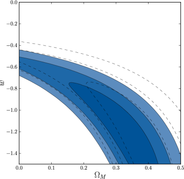
In the cosmology analysis presented here, the statistical errors on have decreased by a significant over the K08 Union analysis, while the estimated systematic errors have only improved by . When combining the SN results with BAO and CMB constraints, statistical errors on have improved by over K08, though the quoted systematic errors have increased . Figure 10 shows a comparison between the constraints from K08 and this compilation in the plane. Even with some improvement on the understanding of systematic errors, it is clear that the dataset is dominated by systematic error (at least at low to mid-).

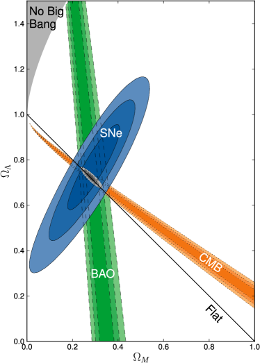
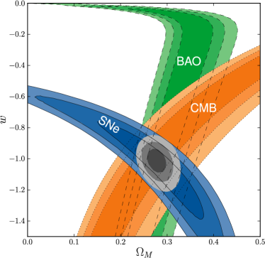
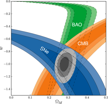
The best fit cosmological parameters for the compilation are presented in Table 8 with constraints from CMB and BAO. The confidence regions in the and planes for the last fit in the table are shown in Figures 11 and 12 respectively.

For the CMB data we implement the constraints from the 7 year data release of the Wilkinson Microwave Anisotropy Probe (WMAP) as outlined in Komatsu et al. (2010). We take their results on (the redshift of last scattering), , and , updating the central values for the cosmological model being considered. Here, is given by
where is the angular distance to , while
Percival et al. (2010) measures the position of the BAO peak from the SDSS DR7 and 2dFGRS data, constraining to , where is the comoving sound horizon and .
For the SNe + BAO fit in Table 8, we add an measurement of km/s/Mpc from Riess et al. (2009), creating a constraint without the CMB that is therefore largely independent of the high-redshift behavior of dark energy (as long as the dark energy density contribution is negligible in the early universe). Note that the constraint relies on most of the nearby supernovae used in this compilation. However, the effect on through from these supernovae is several times smaller than the effect through the Hubble diagram. Alternatively, adding a CMB constraint on of from the WMAP7 webpage101010{http://lambda.gsfc.nasa.gov/product/map/current/params/wcdm_sz_lens_wmap7.cfm} allows us to create a constraint that is independent of . This final result for SNe +BAO+CMB does not improve significantly if the current constraint is added.
8.1. Time variation of the dark energy equation of state
The constraints shown in Figure 12 were obtained assuming that the dark energy equation of state (EOS) is redshift independent. SNe Ia are useful for constraining a redshift dependent since, unlike e.g. CMB, their measured distances at a given redshift are independent of the behavior of dark energy at higher redshifts. A common method to parameterize is
where a cosmological constant is described by . It can be shown (Linder, 2003) that this parameterization provides an excellent approximation to a wide variety of dark energy models. The constraints from the current SN data together with the CMB and BAO data are presented in Figure 13. The flattening of the contours in this diagram at comes from the implicit constraint of matter domination in the early Universe imposed by the CMB and BAO data. Only modest constraints can currently be placed on .
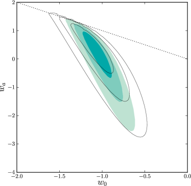
It can be illuminating to study in redshift bins, where is assumed constant in each bin. This method has the advantage that can be studied without assuming a specific form for the relation (Huterer & Starkman, 2003). We carry out the analysis following Kowalski et al. (2008) and fit a constant in each bin, while the remaining cosmological parameters are fit globally for the entire redshift range. Figure 14 shows three such models for the combined constraints from SNe, BAO, CMB, and measurements where we assume a flat Universe. In these scenarios, the measurement does not contribute much, but due to its small improvement on the CMB constraints it gives a small () improvement on the errorbar of the highest redshift bin.
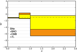
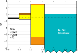
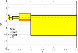
The left panel shows constraints on for three bins. The first bin () shows a well-constrained . The middle bin () shows a poorly-constrained , though one that is distinct from (which would drive to above , resulting in a matter-only universe) at high confidence, indicating the detection of some kind of dark energy in this redshift range. For , there is little constraint on , and only a weak constraint on the existence of dark energy.
The middle panel shows the effect of dividing the highest redshift bin. The constraints on for get much weaker, showing that most of the (weak) constraint on the highest bin in the left panel comes from a combination of the CMB with the well-constrained low-redshift supernova data. Current supernovae at offer no real constraint on . Providing a significant constraint at these redshifts requires significantly better supernova measurements. As in the left panel, in the highest redshift bin is constrained to be less than zero by the requirement from BAO and CMB constraints that the early universe have a matter-dominated epoch.
The right panel shows the effect of dividing the lowest redshift bin. While no significant change in with redshift is detected, there is still considerable room for evolution in , even at low redshift.
Figure 15 shows dark energy density constraints, assuming the same redshift binning as in Figure 14. Note that this is not equivalent to the left and center panels of Figure 14; only in the limit of an infinite number of bins do binned and binned give the same model. Dark energy can be detected at high significance in the middle bin (redshift to ), but there is only weak evidence for dark energy above redshift 1 (left panel). When the bin above redshift 1 is split at a redshift greater than the supernova sample (right panel), it can be seen that the current small sample of supernovae cannot constrain the existence of dark energy above redshift 1.
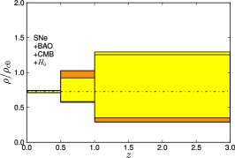

8.2. SNe with ground-based near-IR data
Obtaining near-IR data of SNe Ia, whether from space or from the ground, is critical for constraining the SALT2 color parameter, . Without the near-IR data, the uncertainty in this parameter for 2001hb and 2001gn, both beyond , increases by a factor of two. Precise measurements of are important, since uncertainties in are inflated by and tend to dominate the error budget when the corrected peak -brightness of SNe Ia are calculated.
Both 2001hb and 2001gn were observed with ground-based near-IR instruments. The operational challenges associated in obtaining these data are significant. Long exposure times (ten hours or more taken within a few days) in excellent observing conditions are necessary. Even with queue mode scheduling, these observations are just feasible. Despite the challenges, the uncertainty in the SALT2 color of these two SNe Ia is comparable to the uncertainty in the color of the best space-based measured SNe Ia at .
The ground based near-IR data also allow us to search for systematic offsets with near-IR data taken from space. For SNe Ia observed with NICMOS, the average SALT2 value is mag. By comparison, the weighted average color of the three SNe Ia at with ground-based near-IR data (2001hb and 2001gn from this work, together with 1999fk from Tonry et al. (2003)) that pass the light curve cuts is, . Neither the ground-based or space-based measurements show any Hubble diagram offset, ( and , respectively), from the best fit cosmology. These results include a magnitude dispersion in color, and the fitted systematic dispersions in magnitude. Additional SNe Ia at with ground based near-IR photometry will be published in Suzuki et al. (in preparation) and we will revisit this issue in that paper, where we will also incorporate the results from the NICMOS calibration program referenced in section 7.1.
8.3. Comparison of KeplerCam and SDSS Photometry
H09 and KS09 share three normal supernovae in common: 2005hc, 2005hj, and 2005ir. In comparing the data for these SNe, we noticed that the H09 KeplerCam -band photometry is generally magnitudes fainter than the KS09 SDSS -band photometry based on SALT2 fits including both data sets. The quoted uncertainty is completely dominated by the zero-point uncertainties, as both sets of data have high S/N. The offset is consistent for each supernova. This offset is the correct size and direction to explain the tension in Hubble residuals seen between these datasets in second panel of Figure 8.
SN 2005hc and SN 2005ir were also observed by CSP using the Swope telescope. In these cases, the Swope photometry agrees with the SDSS -band photometry.
9. Summary and Conclusions
We have presented the light curves of SNe Ia in the redshift range . The SNe were discovered as part of a search conducted by the Supernova Cosmology Project using the Subaru, CFHT and CTIO Blanco telescopes in 2001. The fitted light curve shapes and colors at maximum light are all consistent with the corresponding distributions from previous SN surveys.
Following K08, we add these six SNe and other SN Ia data sets to the Union compilation. We have also improved the Union analysis in a number of respects, creating the new Union2 compilation. The most important improvements are: (1) Systematic errors are directly computed using the effect they have on the distance modulus (2) All SN light curves are fitted with the SALT2 light curve fitter.
We determine the best fit cosmology for the Union2 compilation, and the concordance CDM model remains an excellent fit. The new analysis results in a significant improvement over K08 in constraining over the redshift interval . Above , evidence for dark energy is weak. This will remain the case until there is much more high redshift data, with better signal-to-noise and wavelength coverage.
References
- Adelman-McCarthy et al. (2007) Adelman-McCarthy, J. K., et al. 2007, ApJS, 172, 634
- Aguirre (1999) Aguirre, A. 1999, ApJ, 525, 583
- Alard (2000) Alard, C. 2000, A&AS, 144, 363
- Alard & Lupton (1998) Alard, C., & Lupton, R. H. 1998, ApJ, 503, 325
- Amanullah et al. (2003) Amanullah, R., Mörtsell, E., & Goobar, A. 2003, A&A, 397, 819
- Amanullah et al. (2008) Amanullah, R., et al. 2008, A&A, 486, 375
- Anderson & King (2003) Anderson, J., & King, I. R. 2003, PASP, 115, 113
- Appenzeller et al. (1998) Appenzeller, I., et al. 1998, The Messenger, 94, 1
- Astier et al. (2006) Astier, P., et al. 2006, A&A, 447, 31
- Barris et al. (2004) Barris, B. J., et al. 2004, ApJ, 602, 571
- Bergström et al. (2000) Bergström, L., Goliath, M., Goobar, A., & Mörtsell, E. 2000, A&A, 358, 13
- Bessell (1990) Bessell, M. S. 1990, PASP, 102, 1181
- Blondin et al. (2009) Blondin, S., Prieto, J. L., Patat, F., Challis, P., Hicken, M., Kirshner, R. P., Matheson, T., & Modjaz, M. 2009, ApJ, 693, 207
- Bohlin (2007) Bohlin, R. C. 2007, in Astronomical Society of the Pacific Conference Series, Vol. 364, The Future of Photometric, Spectrophotometric and Polarimetric Standardization, ed. C. Sterken, 315–+
- Bohlin (2007) Bohlin, R. C. 2007, Photometric Calibration of the ACS CCD Cameras
- Bohlin & Gilliland (2004) Bohlin, R. C., & Gilliland, R. L. 2004, AJ, 127, 3508
- Cardelli et al. (1989) Cardelli, J. A., Clayton, G. C., & Mathis, J. S. 1989, ApJ, 345, 245
- Conley et al. (2007) Conley, A., Carlberg, R. G., Guy, J., Howell, D. A., Jha, S., Riess, A. G., & Sullivan, M. 2007, ApJ, 664, L13
- Conley et al. (2006) Conley, A., et al. 2006, ApJ, 644, 1
- Conley et al. (2008) Conley, A., et al. 2008, ApJ, 681, 482
- Copin et al. (2006) Copin, Y., et al. 2006, New Astronomy Review, 50, 436
- Cuillandre et al. (2000) Cuillandre, J.-C., Luppino, G., Starr, B., & Isani, S. 2000, Astronomical Telescopes and Instrumentation, 4008, 1010
- D. S. Hayes, L. E. Pasinetti, & A. G. D. Philip (1985) D. S. Hayes, L. E. Pasinetti, & A. G. D. Philip, ed. 1985, IAU Symposium, Vol. 111, Calibration of fundamental stellar quantities; Proceedings of the Symposium, Como, Italy, May 24-29, 1984, ed. D. S. Hayes, L. E. Pasinetti, & A. G. D. Philip
- Dawson et al. (2009) Dawson, K. S., et al. 2009, AJ, 138, 1271
- D’Odorico et al. (1998) D’Odorico, S., Beletic, J. W., Amico, P., Hook, I., Marconi, G., & Pedichini, F. 1998, in Presented at the Society of Photo-Optical Instrumentation Engineers (SPIE) Conference, Vol. 3355, Proc. SPIE Vol. 3355, p. 507-511, Optical Astronomical Instrumentation, Sandro D’Odorico; Ed., ed. S. D’Odorico, 507–511
- Dolphin (2000) Dolphin, A. E. 2000, PASP, 112, 1397
- Dolphin (2009) —. 2009, PASP, 121, 655
- Eisenstein et al. (2005) Eisenstein, D. J., et al. 2005, ApJ, 633, 560
- Ellis et al. (2008) Ellis, R. S., et al. 2008, ApJ, 674, 51
- Fabbro (2001) Fabbro, S. 2001, PhD thesis, l’Université Paris XI Orsay
- Filippenko et al. (2001) Filippenko, A. V., Li, W. D., Treffers, R. R., & Modjaz, M. 2001, in Astronomical Society of the Pacific Conference Series, Vol. 246, IAU Colloq. 183: Small Telescope Astronomy on Global Scales, ed. B. Paczynski, W.-P. Chen, & C. Lemme, 121–+
- Folatelli et al. (2010) Folatelli, G., et al. 2010, AJ, 139, 120
- Foley et al. (2008) Foley, R. J., et al. 2008, ApJ, 684, 68
- Fruchter & Hook (2002) Fruchter, A. S., & Hook, R. N. 2002, PASP, 114, 144
- Fukugita et al. (1996) Fukugita, M., Ichikawa, T., Gunn, J. E., Doi, M., Shimasaku, K., & Schneider, D. P. 1996, AJ, 111, 1748
- Garnavich et al. (1998) Garnavich, P. M., et al. 1998, ApJ, 509, 74
- Goldhaber et al. (2001) Goldhaber, G., et al. 2001, ApJ, 558, 359
- Goobar (2008) Goobar, A. 2008, ApJ, 686, L103
- Goobar et al. (2002) Goobar, A., Bergström, L., & Mörtsell, E. 2002, A&A, 384, 1
- Guy et al. (2007) Guy, J., et al. 2007, A&A, 466, 11
- Guy et al. (2005) Guy, J., Astier, P., Nobili, S., Regnault, N., & Pain, R. 2005, A&A, 443, 781
- Hager (1989) Hager, W. W. 1989, SIAM Rev., 31, 221
- Hamuy et al. (2006) Hamuy, M., et al. 2006, PASP, 118, 2
- Hamuy et al. (1996) Hamuy, M., Phillips, M. M., Suntzeff, N. B., Schommer, R. A., Maza, J., & Aviles, R. 1996, AJ, 112, 2398
- Heyer et al. (2004) Heyer, I., Richardson, M., Whitmore, B., & Lubin, L. 2004, The Accuracy of WFPC2 Photometric Zeropoints
- Hicken et al. (2009a) Hicken, M., et al. 2009a, ApJ, 700, 331
- Hicken et al. (2009b) Hicken, M., Wood-Vasey, W. M., Blondin, S., Challis, P., Jha, S., Kelly, P. L., Rest, A., & Kirshner, R. P. 2009b, ApJ, 700, 1097
- Hodapp et al. (2003) Hodapp, K. W., et al. 2003, PASP, 115, 1388
- Hoeflich et al. (1998) Hoeflich, P., Wheeler, J. C., & Thielemann, F. K. 1998, ApJ, 495, 617
- Holtzman et al. (2008) Holtzman, J. A., et al. 2008, AJ, 136, 2306
- Holz & Linder (2005) Holz, D. E., & Linder, E. V. 2005, ApJ, 631, 678
- Hook et al. (2005) Hook, I. M., et al. 2005, AJ, 130, 2788
- Howell et al. (2007) Howell, D. A., Sullivan, M., Conley, A., & Carlberg, R. 2007, ApJ, 667, L37
- Howell et al. (2005) Howell, D. A., et al. 2005, ApJ, 634, 1190
- Huterer & Starkman (2003) Huterer, D., & Starkman, G. 2003, Physical Review Letters, 90, 031301
- James & Roos (1975) James, F., & Roos, M. 1975, Comput. Phys. Commun., 10, 343
- Jha et al. (2006) Jha, S., et al. 2006, AJ, 131, 527
- Jha et al. (2007) Jha, S., Riess, A. G., & Kirshner, R. P. 2007, ApJ, 659, 122
- Jönsson et al. (2006) Jönsson, J., Dahlén, T., Goobar, A., Gunnarsson, C., Mörtsell, E., & Lee, K. 2006, ApJ, 639, 991
- Kessler et al. (2009) Kessler, R., et al. 2009, ApJS, 185, 32
- Kim & Miquel (2006) Kim, A. G., & Miquel, R. 2006, Astroparticle Physics, 24, 451
- Knop et al. (2003) Knop, R. A., et al. 2003, ApJ, 598, 102
- Komatsu et al. (2010) Komatsu, E., et al. 2010, ArXiv e-prints
- Kowalski et al. (2008) Kowalski, M., et al. 2008, ApJ, 686, 749
- Krisciunas et al. (2005) Krisciunas, K., et al. 2005, AJ, 130, 2453
- Krist (2001) Krist, John E.; Hook, R. N. 2001, The Tiny Tim User’s Guide, STScI
- Kuznetsova et al. (2008) Kuznetsova, N., et al. 2008, ApJ, 673, 981
- Landolt (1992) Landolt, A. U. 1992, AJ, 104, 340
- Law et al. (2009) Law, N. M., et al. 2009, PASP, 121, 1395
- Lentz et al. (2000) Lentz, E. J., Baron, E., Branch, D., Hauschildt, P. H., & Nugent, P. E. 2000, ApJ, 530, 966
- Lidman et al. (2005) Lidman, C., et al. 2005, A&A, 430, 843
- Linder (1988) Linder, E. V. 1988, A&A, 206, 190
- Linder (2003) —. 2003, Physical Review Letters, 90, 091301
- Lupton (2005) Lupton, R. 2005, Transformations between SDSS magnitudes and UBVRcIc, http://www.sdss.org/dr6/algorithms/sdssUBVRITransform.html#Lupton2005
- Ménard et al. (2009a) Ménard, B., Kilbinger, M., & Scranton, R. 2009a, ArXiv e-prints
- Ménard et al. (2008) Ménard, B., Nestor, D., Turnshek, D., Quider, A., Richards, G., Chelouche, D., & Rao, S. 2008, MNRAS, 385, 1053
- Ménard et al. (2009b) Ménard, B., Scranton, R., Fukugita, M., & Richards, G. 2009b, ArXiv e-prints
- Miknaitis et al. (2007) Miknaitis, G., et al. 2007, ApJ, 666, 674
- Miyazaki et al. (2002) Miyazaki, S., et al. 2002, PASJ, 54, 833
- Moorwood et al. (1999) Moorwood, A., Cuby, J. G., & Lidman, C. 1999
- Morokuma et al. (2010) Morokuma, T., et al. 2010, PASJ, 62, 19
- Mörtsell & Goobar (2003) Mörtsell, E., & Goobar, A. 2003, Journal of Cosmology and Astro-Particle Physics, 9, 9
- Muller et al. (1998) Muller, G. P., Reed, R., Armandroff, T., Boroson, T. A., & Jacoby, G. H. 1998, in Society of Photo-Optical Instrumentation Engineers (SPIE) Conference Series, Vol. 3355, Society of Photo-Optical Instrumentation Engineers (SPIE) Conference Series, ed. S. D’Odorico, 577–585
- Nobili et al. (2005) Nobili, S., et al. 2005, A&A, 437, 789
- Nobili et al. (2009) Nobili, S., et al. 2009, ApJ, 700, 1415
- Nobili & Goobar (2008) Nobili, S., & Goobar, A. 2008, A&A, 487, 19
- Nugent et al. (2002) Nugent, P., Kim, A., & Perlmutter, S. 2002, PASP, 114, 803
- Oke et al. (1995) Oke, J. B., et al. 1995, PASP, 107, 375
- Östman & Mörtsell (2005) Östman, L., & Mörtsell, E. 2005, Journal of Cosmology and Astro-Particle Physics, 2, 5
- Patat et al. (2007) Patat, F., et al. 2007, Science, 317, 924
- Percival et al. (2010) Percival, W. J., et al. 2010, MNRAS, 401, 2148
- Perlmutter et al. (1998) Perlmutter, S., et al. 1998, Nature, 391, 51
- Perlmutter et al. (1999) Perlmutter, S., et al. 1999, ApJ, 517, 565
- Perlmutter et al. (1997) Perlmutter, S., et al. 1997, ApJ, 483, 565
- Perlmutter et al. (1995) Perlmutter, S., et al. 1995, ApJ, 440, L41
- Persson et al. (1998) Persson, S. E., Murphy, D. C., Krzeminski, W., Roth, M., & Rieke, M. J. 1998, AJ, 116, 2475
- Phillips (1993) Phillips, M. M. 1993, ApJ, 413, L105
- Raux (2003) Raux, J. 2003, PhD thesis, l’Université Paris XI Orsay
- Regnault et al. (2009) Regnault, N., et al. 2009, A&A, 506, 999
- Riess et al. (1998) Riess, A. G., et al. 1998, AJ, 116, 1009
- Riess et al. (1999) Riess, A. G., et al. 1999, AJ, 117, 707
- Riess et al. (2009) Riess, A. G., et al. 2009, ApJ, 699, 539
- Riess et al. (1996) Riess, A. G., Press, W. H., & Kirshner, R. P. 1996, ApJ, 473, 88
- Riess et al. (2007) Riess, A. G., et al. 2007, ApJ, 659, 98
- Riess et al. (2004) Riess, A. G., et al. 2004, ApJ, 607, 665
- Sasaki (1987) Sasaki, M. 1987, MNRAS, 228, 653
- Schlegel et al. (1998) Schlegel, D. J., Finkbeiner, D. P., & Davis, M. 1998, ApJ, 500, 525
- Schmidt et al. (1998) Schmidt, B. P., et al. 1998, ApJ, 507, 46
- Sheinis et al. (2002) Sheinis, A. I., Bolte, M., Epps, H. W., Kibrick, R. I., Miller, J. S., Radovan, M. V., Bigelow, B. C., & Sutin, B. M. 2002, PASP, 114, 851
- Simon et al. (2009) Simon, J. D., et al. 2009, ApJ, 702, 1157
- Stetson (2000) Stetson, P. B. 2000, PASP, 112, 925
- Stritzinger et al. (2005) Stritzinger, M., Suntzeff, N. B., Hamuy, M., Challis, P., Demarco, R., Germany, L., & Soderberg, A. M. 2005, PASP, 117, 810
- Strovink (2007) Strovink, M. 2007, ApJ, 671, 1084
- Thatte et al. (2009) Thatte, D., Dahlén, T., et al. 2009, NICMOS Data Handbook
- Tonry et al. (2003) Tonry, J. L., et al. 2003, ApJ, 594, 1
- Tripp (1998) Tripp, R. 1998, A&A, 331, 815
- Wang (2005) Wang, L. 2005, ApJ, 635, L33
- Wang et al. (2003) Wang, L., Goldhaber, G., Aldering, G., & Perlmutter, S. 2003, ApJ, 590, 944
- Wang et al. (2008) Wang, X., et al. 2008, ApJ, 675, 626
- Wood-Vasey et al. (2007) Wood-Vasey, W. M., et al. 2007, ApJ, 666, 694
Appendix A Spectra and notes on individual candidates
The spectra of the six SNe in this paper. Details of the spectra for 2001go and 2001gy can be found in Lidman et al. (2005), while the spectrum for 2001cw is described in Morokuma et al. (2010).
The spectrum of each candidate is plotted twice. In the upper panel, the spectrum of the candidate is plotted in the observer frame and is uncorrected for host galaxy light. Telluric absorption features are marked with the symbol . In the lower panel, contamination from the host (if any) is removed, and the resulting spectrum is rescaled and re-binned. This spectrum is plotted in black as a histogram and it is plotted in both the rest frame (lower axis) and the observer frame (upper axis). For comparison, low redshift SNe are plotted as a blue continuous line.
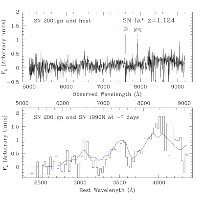
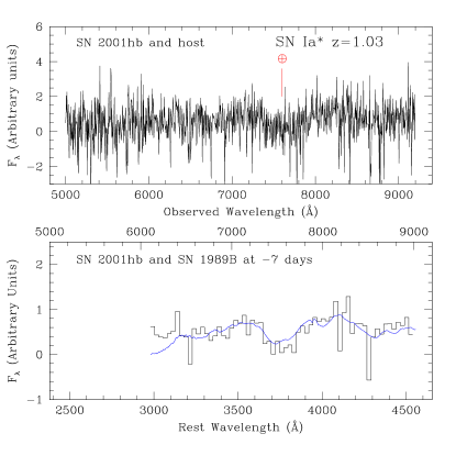

Appendix B Light curve data
Tabulated below are light curve data for the six SNe presented in this paper. The data are listed in chronological order for one SN at a time, and correspond to data points plotted in Figure 6.
All photometry is given as the measured flux, , in the instrumental system, i.e. no color correction (-correction) to a standard system has been applied. The instrumental Vega magnitude may be calculated using the standard formula: , where is the associated zeropoint. For the HST data these are the updated values from Dolphin (2000) given on Andrew Dolphin’s webpage111111{http://purcell.as.arizona.edu/wfpc2_calib/}. The zeropoints have then been converted to by using a gain of . The zeropoints for the ground-based data on the other hand are always given for the photometric reference image, and therefore include exposure time, gain, and for the PSF fitted data, the aperture correction. Note that there are correlated errors between the data points that come from the same light curve build, since the same host galaxy model and zeropoint has been used. This is also reflected by small offsets between different data sets in Figure 6. The covariances are taken into account for the light curve fitting and the full covariance matrices used will be available from the SCP Web site.
The instruments used are as given below. MOSAIC II is the multichip imager on the CTIO 4 m telescope. CFH12k is the multichip imager on the 3.6 m CFHT telescope on Mauna Kea in Hawaii. SuprimeCam is the wide-field imager on the 8.2 m Subaru telescope. SuSI2 is the imager on the NTT 3.6 m telescope at ESO. FORS1 is the imager on the 8 m UT2 (Kueyen) at VLT, ESO. ISAAC and NIRI are the near-infrared imagers on the 8 m UT1 (Antu) at VLT, ESO and Gemini North telescopes respectively. Finally, WFPC2 indicates data obtained with the Planetary Camera CCD and and ACS is the Advanced Camera for Surveys, both on HST.
Note. — This table is published in its entirety in the electronic edition of the Astrophysical Journal. A portion is shown here for guidance regarding its form and content.
Note. — This table is published in its entirety in the electronic edition of the Astrophysical Journal. A portion is shown here for guidance regarding its form and content.
Appendix C Nuisance Parameters as Covariances
Suppose that observations are modeled by , where some of the parameters enter into the model linearly () while some enter non-linearly (). The can be written as
| (C1) |
where is the covariance matrix of the observations, and is the Jacobian matrix of the model with respect to the . Taking the derivative of the and setting it to zero gives the analytic formula for the best-fit
| (C2) |
The likelihoods for the can be found from this restricted parameter space where . Thus, the restricted is given by:
| (C3) | |||||
| (C4) |
with given by
| (C5) | |||||
| (C6) |
In this way, all of the do not have to be explicitly included in the , as long as the weight matrix, , is updated appropriately. Note that may depend on .
C.1. Minimization over and
When errors in the independent variable are present, the true values must be solved for as part of the fit (see discussion in K08). For one supernova, , while the model is given by
| (C7) |
Using ( and are global parameters and cannot be handled one supernova at a time), we have
| (C8) |
The new for this specific example (equation (C4)) is given by equations (4) and (5).
C.2. Minimization over Systematic Errors
Suppose that we have two kinds of measurements: supernova distance measurements ( supernovae), and zeropoint measurements ( zeropoints). The true value of each zeropoint is given by . Because the uncertainties on the supernova distances are unrelated to the uncertainties on the zeropoints,
where is an block and is an block. Similarly, can be split into distances and zeropoints . The model for each supernova distance is given by
| (C9) |
It is derived in the same way as in the previous section, with the substitutions and . The model for the true offset of each zeropoint is simply . Thus,
The upper block of is given by
| (C10) |
none of the other blocks enter into the . Inverting this block (see Hager (1989)) gives:
| (C11) |
Equation (C11) gives us the terms we must add to the supernova distance modulus errors to correctly take the zeropoints into account.