Exact Solution of the Discrete (1+1)–dimensional RSOS Model in a Slit with Field and Wall Interactions

Abstract

We present the solution of a linear Restricted Solid–on–Solid (RSOS) model confined to a slit. We include a field-like energy, which equivalently weights the area under the interface, and also include independent interaction terms with both walls. This model can also be mapped to a lattice polymer model of Motzkin paths in a slit interacting with both walls and including an osmotic pressure.

This work generalises previous work on the RSOS model in the half-plane which has a solution that was shown recently to exhibit a novel mathematical structure involving basic hypergeometric functions ${}_{3}\phi_{2}$. Because of the mathematical relationship between half-plane and slit this work hence effectively explores the underlying $q$-orthogonal polynomial structure to that solution. It also generalises two other recent works: one on Dyck paths weighted with an osmotic pressure in a slit and another concerning Motzkin paths without an osmotic pressure term in a slit.

1 Introduction

Solid–on–Solid (SOS) models describe the interface between low-temperature phases, originally in magnetic systems such as Ising-like models [1, 2], though now more generally. They are effectively directed models in $d+1$ dimensions. The configurations involved in the linear (1+1)–dimensional case, modelling the interface in a two-dimensional system, have also been used to model the backbone of a polymer in solution [3]. The critical phenomena associated with this model describe wetting transitions of the interface with a wall [2]. For the SOS model the phase diagram contains a wetting transition at finite temperature $T_{w}$ for zero field and complete wetting occurs taking the limit $H\to 0$ for $T\geq T_{w}$ [4]. The basic model is naturally described in the half-plane but it is also natural to describe it in the confined geometry of the slit.

The linear SOS model with magnetic field and wall interaction was solved in [4]. Recently the restricted SOS (RSOS), where the interface takes on a restricted subset of configurations, was solved with the same interactions of field and single wall interaction in the half-plane [7]. This has proven to be mathematically quite interesting as both the method of solution and the functions involved were novel. It was found that the solution could be expressed as ratios of linear combinations of terms involving the basic hypergeometric function ${}_{3}\phi_{2}$. Also recently the polymer models of Dyck paths [5] and Motzkin paths [8] in a slit with separate interactions with both surfaces have been considered, without field-like terms. Here the solutions in the slit prove interesting both mathematically and physically. They are of interest physically because the infinite slit limit was shown to be subtly different to the half plane, realising a separate phase diagram [5]. Mathematically the slit exposes the orthogonal polynomial structure of the problem and uncovers hidden combinatorial relationships [8]. Finally, Dyck paths in a slit with wall interactions and weighted by the area under the path, equivalent to a field term in the SOS models, have only recently been analysed [6], and show a rich $q$-orthogonal polynomial structure. To explore further this area of research here we consider the RSOS model in a slit geometry with both separate wall interactions and a field/osmotic pressure term in the energy. We derive the novel $q$-orthogonal polynomials for this problem which give us the exact solution of the generating function.

2 The RSOS model in a slit

The RSOS model we analyse can be described as follows. Consider a two-dimensional square lattice in a slit of width (or thickness) $w\geq 1$. For each column $i$ of the surface a segment of the interface is placed on the horizontal link at height $0\leq r_{i}\leq w$, and successive segments are joined by vertical segments to form a partially directed interface with no overhangs. The configurations are given the energy

$$-\beta E=-K\sum_{i=1}|r_{i}-r_{i-1}|-H\sum_{i=1}r_{i}+B_{0}\sum_{i=1}\delta_{r_{i},0}+B_{w}\sum_{i=1}\delta_{r_{i},w}\;.$$ (2.1)

As in [7], we discuss the RSOS model in terms of lattice paths. An RSOS path is a partially directed self-avoiding path with no steps into the negative $x$-direction and no successive vertical steps. To be precise, an RSOS path of length $N$ with heights $r_{0}$ to $r_{N}$ has horizontal steps at heights $r_{1},\ldots,r_{N}$, and vertical steps between heights $r_{i-1}$ and $r_{i}$ for $i=1,\ldots,N$, but no horizontal step associated with $r_{0}$. This means that an RSOS path starts at height $r_{0}$ with either a horizontal step (if $r_{1}=r_{0}$) or vertical step (if $r_{1}\neq r_{0}$), but must end at height $r_{N}$ with a horizontal step. Figure 1 shows an example.

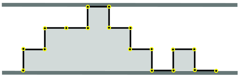
Figure 1: A typical RSOS configuration beginning on the surface and finishing on the surface with a horizontal step: each horizontal step is assigned a weight $x$, each vertical step a weight $y$, each unit of area a weight $q$, each step that touches the bottom surface an additional weight $a$ while each step that touches the top surface an additional weight $b$. The length of the configuration shown here is $N=9$ in a slit of width $w=3$, and the heights are $r_{0}=0$, $r_{1}=1$, $r_{2}=r_{3}=2$, $r_{4}=3$, $r_{5}=2$, $r_{6}=1$, $r_{7}=0$, $r_{8}=1$, and $r_{9}=0$. The weight of this configuration equals $x^{9}y^{8}q^{12}a^{2}b$.

The partition function for the RSOS paths of length $N$ in a slit of width $w\geq 1$ with ends fixed at heights $r_{0}\geq 0$ and $r_{N}\geq 0$, respectively, is given by

$$Z^{w}_{1}(r_{0};r_{1})=\begin{cases}\exp(-\beta E(r_{0};r_{1}))\;,&|r_{0}-r_{1}|\leq 1\\ 0\;,&|r_{0}-r_{1}|>1\;,\end{cases}$$ (2.2)

and

$$Z^{w}_{N}(r_{0};r_{N})=\sum_{\begin{subarray}{c}0\leq r_{1},\ldots,r_{N-1}\leq w\\ |r_{i}-r_{i-1}|\leq 1\end{subarray}}\exp(-\beta E(r_{0};r_{1},\ldots,r_{N}))\;,\qquad N=2,3,\ldots\;,$$ (2.3)

where

$$-\beta E(r_{0};r_{1},\ldots,r_{N})=-K\sum_{i=1}^{N}|r_{i}-r_{i-1}|-H\sum_{i=1}^{N}r_{i}+B_{0}\sum_{i=1}^{N}\delta_{r_{i},0}+B_{w}\sum_{i=1}^{N}\delta_{r_{i},w}\;.$$ (2.4)

Here, we shall consider paths with both ends attached to the surface, i.e. we shall focus on the partition function

$$Z^{w}_{N}=Z^{w}_{N}(0;0)\;.$$ (2.5)

We define

$$y=\exp(-K)\;,\quad q=\exp(-H)\;,\quad a=\exp(B_{0})\;,\quad\mbox{and}\quad b=\exp(B_{w})\;,$$ (2.6)

so $y$ is a temperature–like, $q$ a magnetic field–like and $a$ and $b$ are binding energy–like variables, and write

$$Z^{w}_{N}=Z^{w}_{N}(y,q,a,b)\;.$$ (2.7)

The (reduced) free energy is then

$$\kappa(w;y,q,a,b)=\lim_{N\to\infty}\frac{1}{N}\log Z^{w}_{N}(y,q,a,b)\;.$$ (2.8)

Define the generalised (grand canonical) partition function, or simply generating function, as

$$G_{w}(x,y,q,a,b)=1+\sum_{N=1}^{\infty}x^{N}Z^{w}_{N}(y,q,a,b)\;.$$ (2.9)

Thus, the radius of convergence $x_{c}(w;y,q,a,b)$ of $G^{w}(x,y,q,a,b)$ with respect to the series expansion in $x$ can be identified as $\exp(-\kappa(w;y,q,a,b))$, hence

$$\kappa(w;y,q,a,b)=-\log x_{c}(w;y,q,a,b)\;.$$ (2.10)

It is convenient to consider $G$ as a combinatorial generating function for RSOS paths, where $x$, $y$, $q$, $a$ and $b$ are counting variables for appropriate properties of those paths. Interpreted in such a way, $x$ and $y$ are the weights of horizontal and vertical steps, respectively, $q$ is the weight for each unit of area enclosed by the RSOS path and the $x$-axis, $a$ is an additional weight for each step that touches the bottom surface while $b$ is an additional weight for each step that touches the top surface. For example, the weight of the configuration in Figure 1 is $x^{9}y^{8}q^{12}a^{2}b$.

If we send $w\rightarrow\infty$ then we recover the generating function of the half-plane

$$G^{hp}(x,y,q,a)=1+\sum_{N=1}^{\infty}x^{N}Z^{hp}_{N}(y,q,a)$$ (2.11)

where $Z^{hp}_{N}(y,q,a)=Z^{w}_{N}(y,q,a,b)$ for $w>N$, noting that the paths can have no more vertical steps than horizontal steps in an RSOS path.

We find easily the first few terms of $G^{hp}$ as a series expansion in $x$,

$$G^{hp}(x,y,q,a)=1+ax+(a^{2}+ay^{2}q)x^{2}+\ldots\;,$$ (2.12)

where the constant term corresponds to a zero-step path starting and ending at height zero with weight one.

Note that the radius of convergence of the half-plane generating function $x^{hp}_{c}(y,q,a,b)$ is not a priori the limit of the slit $x_{c}(w;y,q,a,b)$ as was demonstrated in [5] for the corresponding Dyck path problem with $q=1$.

3 Exact solution for the generating function

The key to the solution is a combinatorial decomposition of RSOS paths which leads to a functional equation for the generating function $G_{w}$. This decomposition is done with respect to the left-most horizontal step touching the surface at height zero, and is shown diagrammatically in Figure 2.

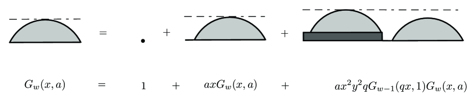
Figure 2: The diagrammatic form of the functional equations for RSOS paths, indicating the combinatorial decomposition of RSOS paths.

We distinguish three cases:

• The RSOS path has zero length, and there is no horizontal step at height zero. The contribution to the generating function is $1$.

• The RSOS path starts with a horizontal step, which therefore is at height zero. The rest of this path is again a RSOS path. The contribution to the generating function is $\kappa xG_{w}(x,y,q,\kappa)$.

• The RSOS path starts with a vertical step. Then there will be a left-most horizontal step at height zero, and removing this step cuts the path into two pieces. The left path starts with a vertical and horizontal step, followed by an RSOS path starting and ending at height one and not touching the surface, followed by a vertical step to height zero. This left path is effectively in a slit of width $w-1$. The right path is again a RSOS path in the slit of width $w$. The contribution to the generating function is $yxqG_{w-1}(qx,y,q,1)y\kappa xG_{w}(x,y,q,\kappa)$.

Put together, this decomposition leads to a functional-recurrence equation for the generating function

$$G_{w}(x,y,q,a,b)=1+axG_{w}(x,y,q,a,b)+aqx^{2}y^{2}G_{w-1}(qx,y,q,1,b)G_{w}(x,y,q,a,b)\;,$$ (3.1)

with “initial condition”

$$G_{0}(x,y,q,a,b)=\frac{b}{1-abx}\;.$$ (3.2)

If we send $w\rightarrow\infty$ then we recover the functional equation of the half-plane

$$G^{hp}(x,y,q,a)=1+axG^{hp}(x,y,q,a)+aqx^{2}y^{2}G^{hp}(qx,y,q,1)G^{hp}(x,y,q,a)\;.$$ (3.3)

whose solution is given in [7].

We can rewrite (3.1) as

$$G_{w}(x,y,q,a,b)=\frac{1}{1-ax-aqx^{2}y^{2}G_{w-1}(qx,y,q,1,b)}\;,$$ (3.4)

For general values of $q$, a formal iteration of (3.4) leads to a continued fraction expansion

$$G_{w}(x,y,q,a,b)=\cfrac{1}{1-ax-\cfrac{aqx^{2}y^{2}}{1-qx-\cfrac{q^{3}x^{2}y^{2}}{1-q^{2}x-\cfrac{q^{5}x^{2}y^{2}}{1-q^{3}x-\cfrac{q^{7}x^{2}y^{2}}{\genfrac{}{}{0.0pt}{}{}{\ddots\genfrac{}{}{0.0pt}{}{}{\genfrac{}{}{0.0pt}{}{}{\genfrac{}{}{0.0pt}{}{}{\cfrac{}{1-q^{w-1}x-\cfrac{bq^{2w-1}x^{2}y^{2}}{1-bq^{w}x}}}}}}}}}}}\;.$$ (3.5)

However, there is a non-trivial method to solve the functional equation for $G$ as a ratio of $q$-orthogonal polynomials. It is clear that the generating function can be written as a rational function

$$G_{w}(x,y,q,a,b)=\frac{P_{w}(x,y,q,a,b)}{Q_{w}(x,y,q,a,b)}$$ (3.6)

though it does not simply follow to write expressions for these. It does however follow from the theories of continued fractions and orthogonal polynomials (see pages 256–257 of Andrews, Askey and Roy [9]) that both the numerator $P_{w}$ and denominator $Q_{w}$ of the generating function satisfy recursions

$$P_{w}(x,y,q,a,b)=\begin{cases}b\;,&w=0\\ 1-bqx\;,&w=1\\ (1-bq^{w}x)P_{w-1}(x,y,q,a,1)-bq^{2w-1}x^{2}y^{2}P_{w-2}(x,y,q,a,1)\;&w\geq 2\end{cases}$$ (3.7)

and

$$Q_{w}(x,y,q,a,b)=\begin{cases}1-abx\;,&w=0\\ 1-bqx-ax(1-bqx(1-y^{2}))\;,&w=1\\ -bq^{w}xQ_{w-1}(x,y,q,a,1)-bq^{2w-1}x^{2}y^{2}Q_{w-2}(x,y,q,a,1)\;&w\geq 2\;.\end{cases}$$ (3.8)

So it is the functions $Q_{w}(x,y,q,a,b)$ that are the $q$-orthogonal polynomials referred to in the Introduction.

One can immediately note that

$$P_{w}(x,y,q,a,b)=Q_{w}(x,y,q,0,b)$$ (3.9)

so that

$$G_{w}(x,y,q,a,b)=\frac{Q_{w}(x,y,q,0,b)}{Q_{w}(x,y,q,a,b)}\;.$$ (3.10)

We now form the width generating function for the denominator as

$$W(t,x,y,q,a,b)=\sum_{w=0}^{\infty}Q_{w}(x,y,q,a,b)t^{w}$$ (3.11)

and find a functional equation for $W(t)$ from the recurrence (3.8) as

$$W(t,x,y,q,a,b)=1 -abx-abqx^{2}y^{2}t+tW(t,x,y,q,a,1)$$ (3.12)

$$-bqxtW(qt,x,y,q,a,1)-bq^{3}x^{2}y^{2}t^{2}W(q^{2}t,x,y,q,a,1)$$

Unlike in the case of Dyck paths in a slit [6], one cannot solve for $W(t)\equiv W(t,x,y,q,a,1)$ by direct iteration, as the functional equation involves $W(t)$, $W(qt)$, and $W(q^{2}t)$. So let us return to $Q_{w}(x,y,q,a,b)$ and consider the case $b=1$, as this is all that is required to find the full solution. Let

$$R_{w}\equiv Q_{w}(x,y,q,a,1)\;.$$ (3.13)

From the recurrence (3.8) we have for $w\geq 2$ that

$$R_{w}=(1-q^{w}x)R_{w-1}-q^{2w-1}x^{2}y^{2}R_{w-2}$$ (3.14)

with initial conditions

$$R_{0}= \;1-ax\;,$$ (3.15)

$$R_{1}= \;1-qx-ax(1-bqx(1-y^{2}))\;.$$

Attempting to mimic aspects of the half-plane solution [7], we define $S_{w}$ via

$$R_{w}=(-1)^{w}q^{w(w+1)/2}x^{w}S_{w}\;.$$ (3.16)

This gives us the recurrence

$$q^{w}x(S_{w}-S_{w-1}+y^{2}S_{w-2})+S_{w-1}=0$$ (3.17)

with initial conditions

$$S_{0}= \;1-ax\;,$$ (3.18)

$$-qxS_{1}= \;1-qx-ax(1-bqx(1-y^{2}))\;.$$

Continuing with inspiration from the half-plane solution [7], we try the Ansatz

$$S_{w}=\mu^{w}\sum_{n=0}^{\infty}c_{n}q^{-nw}\;.$$ (3.19)

For $n=0$ we have

$$x(\mu^{2}-\mu+y^{2})c_{0}=0$$ (3.20)

and for $n>0$ we have

$$c_{n}=-\frac{\mu q^{n}c_{n-1}}{(y^{2}q^{2n}-\mu q^{n}+\mu^{2})qx}$$ (3.21)

This implies that $\mu$ satisfies

$$\mu^{2}-\mu+y^{2}=0$$ (3.22)

for our Ansatz to work. We now parametrise $y$ via

$$y^{2}=\lambda(1-\lambda)$$ (3.23)

which changes (3.20) into

$$x(\mu-\lambda)(\mu-1+\lambda)c_{0}=0$$ (3.24)

and the recurrence into

$$c_{n}=-\frac{\mu q^{n}c_{n-1}}{(\mu-\lambda q^{n})(\mu-(1-\lambda)q^{n})qx}$$ (3.25)

We see immediately that either $\mu=\lambda$ or $\mu=1-\lambda$ and that we have two solutions from our Ansatz. This leads to the general solution for $S_{w}$ as

$$S_{w}=A\lambda^{w} \sum_{n=0}^{\infty}\left(-\frac{1}{x}\right)^{n}q^{-nw}\prod_{k=0}^{n-1}\frac{q^{k}}{(1-q^{k+1})(\lambda-(1-\lambda)q^{k+1})}$$ (3.26)

$$+B(1-\lambda)^{w} \sum_{n=0}^{\infty}\left(-\frac{1}{x}\right)^{n}q^{-nw}\prod_{k=0}^{n-1}\frac{q^{k}}{(1-q^{k+1})((1-\lambda)-\lambda q^{k+1})}\;,$$

and so for $R_{w}$ via (3.16). One can then use the initial conditions (3.15) to solve for the coefficients $A$ and $B$.

Defining

$$\phi^{(N)}_{w}\left(\rho,q\right)=\sum_{n=0}^{N}\frac{\rho^{n}q^{(n-N-w+1)n}}{(q;q)_{n}(q;q)_{N-n}(\rho q;q)_{n}(\frac{q}{\rho};q)_{N-n}}$$ (3.27)

where

$$(t;q)_{n}=\prod_{k=0}^{n-1}(1-tq^{k})$$ (3.28)

is the standard $q$-product, after some lengthy calculations one finds

$$Q_{w}(x,y,q,a,1)=q^{w(w+1)/2}\left[(1-ax)T^{(1)}_{w}(x,q,\lambda)+(1-qx-ax(1-y^{2}))T^{(2)}_{w}(x,q,\lambda)\right]$$ (3.29)

with

$$T^{(1)}_{w}(x,q,\lambda)=\frac{1}{1-2\lambda}\times\\ \sum_{N=0}^{w}q^{(N^{2}-3N)/2}(-x)^{w-N}\left[\frac{\lambda^{w}}{(1-\lambda)^{N-1}}\phi^{(N)}_{w}\left(\frac{1-\lambda}{\lambda},q\right)-\frac{(1-\lambda)^{w}}{\lambda^{N-1}}\phi^{(N)}_{w}\left(\frac{\lambda}{1-\lambda},q\right)\right]$$ (3.30)

and

$$T^{(2)}_{w}(x,q,\lambda)=-\frac{1}{1-2\lambda}\times\\ \sum_{N=0}^{w}q^{(N^{2}-N-1)/2}(-x)^{w-1-N}\left[\frac{\lambda^{w}}{(1-\lambda)^{N}}\phi^{(N)}_{w+1}\left(\frac{1-\lambda}{\lambda},q\right)-\frac{(1-\lambda)^{w}}{\lambda^{N}}\phi^{(N)}_{w+1}\left(\frac{\lambda}{1-\lambda},q\right)\right]\;.$$ (3.31)

To obtain an expression for $G_{w}$ one can then substitute (3.29) into (3.8) to obtain an expression for $Q_{w}(x,y,q,a,b)$ and then this into (3.10) to give $G_{w}(x,y,q,a,b)$.

4 The infinite width limit

For any finite length the partition function in the slit becomes equal to the half-plane for large enough widths $w$. This means that the generating functions $G_{w}$ approach $G^{hp}$, when they converge. The half-plane solution can be found in [7]. Here we take the limit $w\rightarrow\infty$ of the solution derived for finite width. This gives us a more compact expression for the denominator of the $G^{hp}$ than appears in [7].

After some work we find, using $\hat{\lambda}=1-\lambda$,

$$Q^{hp}(x,y,q,a)=(1-ax)\left[P^{(1)}(x,q,\lambda)+P^{(2)}(x,q,\lambda)\right]+(1-qx-ax(1-y^{2}))\left[P^{(3)}(x,q,\lambda)+P^{(4)}(x,q,\lambda)\right]$$ (4.1)

with

$$P^{(1)}(x,q,\lambda)=\sum_{M=0}^{\infty}\sum_{m=0}^{\infty}\frac{(-x)^{M}\,\lambda^{M+m}\,\hat{\lambda}^{1-m}\,q^{\frac{1}{2}M^{2}+Mm+m^{2}+\frac{1}{2}M-m}}{(\hat{\lambda}-\lambda)(q;q)_{\infty}(q;q)_{m}({\lambda q}/{\hat{\lambda}};q)_{m}({\hat{\lambda}q}/{\lambda};q)_{\infty}}\;,$$ (4.2)

$$P^{(2)}(x,q,\lambda)=\sum_{M=0}^{\infty}\sum_{m=0}^{\infty}\frac{(-x)^{M}\,\lambda^{1-m}\,\hat{\lambda}^{m+M}\,q^{\frac{1}{2}M^{2}+Mm+m^{2}+\frac{1}{2}M-m}}{(\lambda-\hat{\lambda})(q;q)_{\infty}(q;q)_{m}({\lambda q}/{\hat{\lambda}};q)_{\infty}({\hat{\lambda}q}/{\lambda};q)_{m}}\;,$$ (4.3)

$$P^{(3)}(x,q,\lambda)=\sum_{M=0}^{\infty}\sum_{m=0}^{\infty}\frac{(-x)^{M}\,\lambda^{M+m+1}\,\hat{\lambda}^{-m}\,q^{\frac{1}{2}M^{2}+Mm+m^{2}+\frac{3}{2}M+m}}{(\lambda-\hat{\lambda})(q;q)_{\infty}(q;q)_{m}({\lambda q}/{\hat{\lambda}};q)_{m}({\hat{\lambda}q}/{\lambda};q)_{\infty}}\;,$$ (4.4)

and

$$P^{(4)}(x,q,\lambda)=\sum_{M=0}^{\infty}\sum_{m=0}^{\infty}\frac{(-x)^{M}\,\lambda^{-m}\,\hat{\lambda}^{M+m+1}\,q^{\frac{1}{2}M^{2}+Mm+m^{2}+\frac{1}{2}M-m}}{(\hat{\lambda}-\lambda)(q;q)_{\infty}(q;q)_{m}({\lambda q}/{\hat{\lambda}};q)_{m}({\hat{\lambda}q}/{\lambda};q)_{\infty}}\;.$$ (4.5)

As in [7], we then find

$$G^{hp}(x,y,q,a)=\frac{Q^{hp}(x,y,q,0)}{Q^{hp}(x,y,q,a)}\;.$$ (4.6)

While this expression is equivalent to that found in [7], we note that its structure is fundamentally different.

5 Mapping to Motzkin paths polymer model

As foreshadowed in the Introduction there is a mapping between RSOS configurations and Motzkin paths. Starting at the leftmost site one uses the mapping in Figure 3 to construct a Motzkin path from an RSOS configuration.

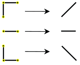
Figure 3: The mapping from RSOS paths to Motzkin paths.

For example, the mapping of configuration in Figure 1 can be seen in Figure 4.

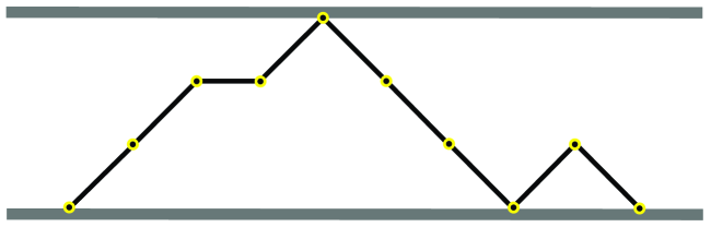
Figure 4: The mapping of RSOS configuration in Figure 1 to a Motzkin path.

This implies that the generating function we have found is also that of of Motzkin paths in a slit weighted by area (which can be used to model an osmotic pressure [6]) an interaction with both walls. In this way the current work is a generalisation of that found in [6].

6 Conclusion

In this paper we have presented a solution to the linear RSOS model in a slit with field and wall interaction terms in the energy. In particular we have evaluated the generating function and demonstarted that its limit is the half-plane solution found earlier. The numerator and denominator polynomials of the slit generating function are novel $q$-orthogonal polynomials associated with the continued fraction expansion of the half-plane solution.

References

• [1] H. N. V. Temperley, Proc. Camb. Phil. Soc. 48, 638 (1952).
• [2] S. Dietrich, in Phase Transitions and Critical Phenomena, Vol. 12, ed. by C. Domb and J. L. Lebowitz, (Academic Press, London, 1988).
• [3] V. Privman and N. M. Švrakić, Lecture Notes in Physics 338 (Springer–Verlag, Berlin, 1989).
• [4] A. L. Owczarek and T. Prellberg, J. Stat. Phys. 70 1175 (1993)
• [5] R. Brak, A.L. Owczarek, A. Rechnitzer and S.G. Whittington J. Phys. A: Math. Gen., 38: 4309, (2005).
• [6] A. L. Owczarek and T. Prellberg, A simple model of a vesicle drop in a confined geometry, submitted to JSTAT (2010).
• [7] A. L. Owczarek and T. Prellberg, J. Phys. A: Math. Gen., 42: 495003, (2009).
• [8] R. Brak, G.K. Iliev, A. Rechnitzer and S.G. Whittington J. Phys. A: Math. Theor., 40, 4415, (2007).
• [9] G. E. Andrews, R. Askey, and R. Roy, volume 71 of Encyclopedia of Mathematics and its Applications, Cambridge University Press, Cambridge, 1999.