Random Ancestor Trees

Abstract

We investigate a network growth model in which the genealogy controls the evolution. In this model, a new node selects a random target node and links either to this target node, or to its parent, or to its grandparent, etc; all nodes from the target node to its most ancient ancestor are equiprobable destinations. The emerging random ancestor tree is very shallow: the fraction $g_{n}$ of nodes at distance $n$ from the root decreases super-exponentially with $n$, $g_{n}=e^{-1}/(n-1)!$. We find that a macroscopic hub at the root coexists with highly connected nodes at higher generations. The maximal degree of a node at the $n$th generation grows algebraically as $N^{1/\beta_{n}}$ where $N$ is the system size. We obtain the series of nontrivial exponents which are roots of transcendental equations: $\beta_{1}\cong 1.351746$, $\beta_{2}\cong 1.682201$, etc. As a consequence, the fraction $p_{k}$ of nodes with degree $k$ has algebraic tail, $p_{k}\sim k^{-\gamma}$, with $\gamma=\beta_{1}+1=2.351746$.

I Introduction

The interplay between dynamics, structure, and function of complex networks is the subject of intense current research ws ; ab ; dm ; bbv . A wide spectrum of social, technical, and biological networks have broad degree distributions with a power-law tail ab ; dm . Further, many real-life networks also have macroscopic hubs that are connected to a finite fraction of all nodes and these hubs play important function in the network ab ; dm ; bbv . In this study, we introduce a minimal model that captures both of these features.

Common mechanisms of network growth include preferential attachment yule ; simon ; ba ; krl ; dms , copying, and re-direction kum ; kr ; la ; kr2 . In these processes, a target node is identified and the attachment is either to the target node itself or to one of its immediate ancestors. These growth processes result in heterogeneous networks with broad degree distributions. However, there are no macroscopic hubs because the maximal degree in these networks grows sub-linearly with the network size.

In this study, we consider the complementary situation where attachment to any ancestor is possible. We show that the resulting network has a fundamentally different structure: there is coexistence between a hub with a macroscopic degree and highly connected nodes with sub-macroscopic degrees. Moreover, there is a series of exponents that characterize how the maximal degree at a given distance from the root scales with system size.

Figure 1: The random ancestor tree. A new node attaches, with equal probabilities, to one of three nodes: the target node (marked by $\times$), its parent, or its grandparent.

To model situations where the genealogy controls the network growth, we start with a single node, the root, and add nodes sequentially, so that each new node attaches to an existing node through a two-step process (see Fig. 1):

• The new node selects a target node at random.

• The new node attaches to one node, selected at random from the set of nodes that includes the target node and all its ancestors.

Since each new node adds a single link, the growing network retains a tree structure, and apart from the root, each node has a single parent node. We term the resulting structure the random ancestor tree. An appealing feature of this model is the absence of control parameters.

Our motivation for this model comes from social, scholarly, and reference networks wf . For example, the published literature in science, law, and religion grows by sequential addition of material. Starting with some reference, a scholar typically studies an entire line of preceding reports or rulings, and refers to the most appropriate or the most important published literature, not necessarily the most recent one sr ; mejn ; rfmv . In this sense, the evolution of such reference networks is coupled to their genealogy.

We find that the random ancestor tree has a single macroscopic hub, namely the root, that is connected to a fraction $e^{-1}$ of all nodes. Furthermore, the degree distribution is broad as the fraction $p_{k}$ of nodes with degree $k$ decays algebraically,

$$p_{k}\sim k^{-\gamma},\qquad\gamma=2.351746,$$ (1)

when $k\to\infty$. Interestingly, the exponent $\gamma$ is obtained as a root of a transcendental equation. We also obtain a series of nontrivial exponents $\gamma_{n}$, each characterizing the degree distribution of nodes at the $n$th generation. As $n$ increases, the exponents $\gamma_{n}$ increase, so that the nodes become less and less connected as their distance from the root increases.

Throughout this paper, we focus on the asymptotic behavior of large trees. We first analyze the genealogical structure of the random ancestor tree in section II. The depth distribution indicates that the root is a macroscopic hub, and in section III we show that the root is the only such hub. We then establish (Sec. IV) the degree of the most connected nodes at higher generations and discuss the implications of these results for the degree distribution (Sec. V). Other structural properties including the number of leaves, and the likelihood that the tree has star or chain topology are derived in section VI. Conclusions are given in section VII.

II Genealogical Structure

We treat the random ancestor tree as a genealogical tree and group nodes according to generation (figure 1). The first generation consists of nodes at distance one from the root, the second generation includes nodes at distance two from the root, etc. In principle, the number of nodes in each generation fluctuates from one realization to another, yet in the thermodynamic limit such fluctuations are negligible, and we therefore study the average number of nodes in each generation.

Let $N$ be the total number of nodes in the tree and let $G_{n}(N)$ be the average number of nodes at distance $n$ from the root. Only the root belongs to the zeroth generation and therefore, $G_{0}(N)=1$. The average number of nodes in the first generation, $G_{1}(N)$, grows according to the rate equation

$$\frac{dG_{1}}{dN}=\frac{G_{0}}{N}+\frac{G_{1}}{2N}+\frac{G_{2}}{3N}+\cdots.$$ (2)

Hereinafter we treat the size of the network $N$ as a continuous variable; our results are asymptotically exact in the limit $N\to\infty$. Equation (2) reflects that new nodes are added to the first generation only when a new node links to the root. The first term on the right-hand side corresponds to the situation when the root is chosen as the target node; the second term accounts for situations when a node in the first generation is chosen — then the probability that the actual link will be to the root is 1/2; the following terms describe situations where the target nodes are in higher generations.

The generalization of (2) to arbitrary generation $n$ is straightforward,

$$\frac{dG_{n}}{dN}=\sum_{i\geq n}\frac{G_{i-1}}{i\,N}.$$ (3)

We now introduce $g_{n}$, the fraction of nodes that belong to the $n$th generation,

$$G_{n}(N)=g_{n}N.$$ (4)

The coefficients $g_{n}$ are normalized, $\sum_{n\geq 1}g_{n}=1$. Further, since $G_{0}=1$ we have $g_{0}=0$ in the limit $N\to\infty$. Equation (3) shows that the fractions $g_{n}$ satisfy

$$g_{n}=\sum_{i\geq n}i^{-1}g_{i-1}\,.$$ (5)

It is convenient to re-write Eq. (5) as the explicit recursion

$$g_{n}=n^{-1}g_{n-1}+g_{n+1}\,.$$ (6)

By evaluating the first few terms, $g_{2}=g_{1}$, $g_{3}=g_{1}/2!$, $g_{4}=g_{1}/3!$, and by induction, $g_{n}=g_{1}/(n-1)!$. The normalization condition $\sum_{n\geq 1}g_{n}=1$ sets $g_{1}=e^{-1}$. Thus,

$$g_{n}=\frac{e^{-1}}{(n-1)!},$$ (7)

indicating that the number of nodes decays super-exponentially with increasing generation or alternatively, depth. Hence, the random ancestor tree is exceptionally shallow. For instance, the average depth is finite: $\langle n\rangle=\sum_{n\geq 1}ng_{n}=2$.

The genealogical structure of the random ancestor tree drastically differs from the genealogical structure of other growing networks kr . In particular, random recursive trees hmm ; krb , which grow by attachment of new nodes to random target nodes, have the depth distribution $G_{n}(N)=(\ln N)^{n}/n!$. Thus, there is a sharp peak at $n_{\rm peak}\sim\ln N$, and furthermore, the maximal depth, defined as the deepest non-empty generation $n_{\rm max}$, also scales logarithmically with system size, $n_{\rm max}\sim\ln N$ kr . This behavior is very robust and occurs in most growing trees bp ; nsw ; bo , but there are exceptions where the maximal depth grows algebraically with system size dkm .

For the random ancestor tree, the generation profile (7) is a sharply decreasing function of depth, and from the criterion $G_{n_{\rm max}}\sim 1$ we estimate the maximal depth

$$n_{\rm max}\approx\frac{\ln N}{\ln(\ln N)}\,.$$ (8)

This depth behavior reflects that the tree is shallow bk .

III Macroscopic Hub

The random ancestor tree has a macroscopic hub: the root is connected to a finite fraction, $e^{-1}=0.367879$, of all nodes as follows from (7). Such macroscopic hubs are found in social networks wf , and have an important function in as transportation networks bbv ; ab1 ; yb ; gm ; wrd . Yet, with a few exceptions including super-linear preferential attachment krl ; kr ; kk , most models of network growth have no such hubs and instead, the most central nodes have degrees that grow sub-linearly with network size.

To find out whether, in addition to the root, there are other hubs, let’s consider the most connected node at the first generation. We denote the number of descendants of this node in the second generation by $H_{2}(N)$, the number of its descendants in the third generation by $H_{3}(N)$, etc. The equation governing $H_{j}(N)$ is identical to (3),

$$\frac{dH_{j}}{dN}=\sum_{i\geq j}\frac{H_{i-1}}{i\,N}\,,$$ (9)

with $H_{1}=1$. By definition, the node degree is $1+H_{2}(N)$.

Suppose that the most connected node at the first generation has macroscopic degree, $H_{2}\sim N$. Since $dH_{3}/dN>H_{2}/(3N)$ then $H_{3}\sim N$ as well. In general,

$$H_{j}(N)=u_{j}N$$ (10)

for all $j\geq 2$. By substituting (10) into (9), we find that the coefficients $u_{j}$ satisfy a recursion relation identical to (6),

$$u_{j}=j^{-1}u_{j-1}+u_{j+1}.$$ (11)

Any solution to (11) is a linear combination of the two independent solutions: the fast-decaying solution above $u_{j}=1/(j-1)!$ and the slow-decaying one, $u_{j}\sim j^{-1}$ when $j\gg 1$. For the first few coefficients we have $u_{1}=0$ and $u_{2}=u_{3}$. The boundary condition $u_{1}=0$ implies that we can not express the solution solely in terms of the rapidly decaying solution $u_{j}=1/(j-1)!$. Yet, the slowly decaying solution is unphysical because the sum $\sum_{j}u_{j}$ diverges. Therefore, the only possible solution is the trivial one, $u_{j}=0$ for all $j\geq 1$, and we conclude that there are no macroscopic hubs in the first generation.

Similarly, there are no macroscopic hubs in higher generations. If there is a hub in the $n$th generation, the recurrence (11) holds for $j>n$ with the boundary condition $u_{n}=0$, or equivalently $u_{n+1}=u_{n+2}$. By repeating the steps above, we conclude that all coefficients $u_{j}$ vanish.

IV Highly Connected Nodes

In the previous section we have shown that the degree of the most connected node in the first generation cannot be macroscopic. It is then natural to assume that the degree scales as $N^{1/\beta}$ with $\beta>1$, or equivalently OK

$$H_{j}=H_{2}\,h_{j},\quad{\rm with}\quad H_{2}\simeq C\,N^{1/\beta},$$ (12)

for all $j\geq 2$. The fractions $h_{j}$ satisfy

$$h_{j}=\beta\,\sum_{i\geq j}i^{-1}h_{i-1}\,,$$ (13)

obtained by substituting (12) into (9). Therefore, the recursion relation (6) becomes

$$h_{j}=\beta\,j^{-1}h_{j-1}+h_{j+1}.$$ (14)

The boundary conditions is

$$h_{1}=0,\quad h_{2}=1.$$ (15)

Certain features can be determined without solving Eqs. (14)–(15). For instance, to obtain the total number of descendants $h_{\rm tot}=\sum_{i\geq 2}h_{i}$ we multiply (14) by $j$ and sum over all $j$. This yields

$$h_{\rm tot}=\frac{1}{\beta-1}\,.$$ (16)

Since $h_{\rm tot}>1$, we have the bound $\beta<2$.

Similarly, by multiplying (14) by $j^{2}$ and summing over all $j$ we determine the average generation number

$$\langle\,j\,\rangle=\frac{\sum_{j\geq 2}jh_{j}}{\sum_{j\geq 2}h_{j}}=\frac{2}{2-\beta}\,.$$

The second order linear difference equation (14) has two independent solutions. We obtain the asymptotic behavior of these solutions by converting the difference equation (14) into a differential equation. If $h_{j}$ decays sufficiently slow, we may approximate Eq. (14) by the differential equation $dh/dj\simeq-\beta\,h/j$ with solution $h_{j}\sim j^{-\beta}$ at large $j$. Otherwise, if $h_{j}$ decays very quickly, we have $h_{j}\simeq\beta\,h_{j-1}/j$ in the leading order and therefore $h_{j}\sim\beta^{j}/j!$. Using this solution as an integrating factor, that is, substituting $h_{j}=q_{j}\,\beta^{j}/j!$ into Eq. (14), we have the recurrence $q_{j}-q_{j-1}=\beta q_{j+1}/(j+1)$. This recurrence reduces to the differential equation $dq/dj\simeq\beta\,q/j$, with power-law solution $q_{j}\sim j^{\beta}$. Therefore the asymptotic behavior of the second solution to Eq. (14) is

$$h_{j}\sim\frac{j^{\beta}\,\beta^{j}}{j!}.$$ (17)

Equations (14)–(15) admit a solution for arbitrary value of $\beta$. In general, such a solution is a linear combination of the two solutions above. However, the slowly decaying solution is unphysical. If $H_{j}\sim j^{-\beta}N^{1/\beta}$ for $j\gg 1$, then the depth of the subtree emanating from the most connected node in the first generation, $j_{\rm max}\sim N^{1/\beta^{2}}$, as follows from the criterion $H_{j_{\rm max}}\sim 1$, would exceed the maximal depth (8). Therefore, we must find the special value of $\beta$ for which solution to (14)–(15) is the rapidly decaying solution with the asymptotic behavior (17). Therefore, $\beta$ is analogous to an eigenvalue.

To determine the proper eigenvalue $\beta$ we use the generating function technique. We write

$$\mathcal{H}(z)=\sum_{j\geq 2}h_{j}z^{j}$$ (18)

and convert the difference equation (14) into an integral equation

$$\mathcal{H}(z)=\beta\int_{0}^{z}dx\,\mathcal{H}(x)+\frac{\mathcal{H}(z)-z^{2}}{z}.$$ (19)

Note that $\mathcal{H}(z)=z^{2}+z^{3}+\cdots$ for small $z$ and in addition, Eq. (16) sets $\mathcal{H}(1)=h_{\rm tot}=(\beta-1)^{-1}$.

Given the form of Eq. (19), we focus on the integral of the generating function, $\mathcal{F}(z)=\int_{0}^{z}dx\,\mathcal{H}(x)$, and convert the integral equation (19) into the differential equation

$$\frac{d\mathcal{F}}{dz}+\beta\,z\,(1-z)^{-1}\mathcal{F}=z^{2}(1-z)^{-1}.$$ (20)

The boundary condition is $\mathcal{F}(0)=0$. We use the integrating factor $I(z)=e^{-\beta\,z}(1-z)^{-\beta}$ to simplify (20) to $d(\mathcal{F}I)/dz=z^{2}(1-z)^{-1}I$. Hence, the solution of (20) is

$$\mathcal{F}(z)=e^{\beta(z-1)}(1-z)^{\beta}\int_{0}^{z}dx\,e^{\beta(1-x)}\,\frac{x^{2}}{(1-x)^{1+\beta}}\,.$$ (21)

The behavior of the generating function in the limit $z\to 1$ reflects the behavior of the coefficients $h_{j}$ in the limit $j\to\infty$. Therefore, we evaluate the integral in (21) in the limit $z\to 1$,

$$\int_{0}^{z}dx\,e^{\beta(1-x)}\,x^{2}\,(1-x)^{-1-\beta}$$

$$= \int_{0}^{z}dx\,e^{\beta(1-x)}\left[1-2(1-x)+(1-x)^{2}\right](1-x)^{-1-\beta}$$

$$= \int_{1-z}^{1}dy\,e^{\beta y}[y^{-1-\beta}-2y^{-\beta}+y^{1-\beta}]$$

$$= \sum_{k=0}^{\infty}\frac{\beta^{k}}{k!}\int_{1-z}^{1}dy\,\left[y^{k-1-\beta}-2y^{k-\beta}+y^{k+1-\beta}\right]$$

$$\simeq f(\beta)+(1-z)^{-\beta}\left[\frac{1}{\beta}-\frac{2-\beta}{\beta-1}(1-z)\right].$$

The function $f(\beta)$ is given by the infinite sum

$$f(\beta)=\sum_{k=0}^{\infty}\frac{\beta^{k}}{k!}\left(\frac{1}{k-\beta}-\frac{2}{k+1-\beta}+\frac{1}{k+2-\beta}\right).$$

We can also express this function in terms of the incomplete Gamma function $\gamma(a,x)=\int_{0}^{x}dt\,t^{a-1}\,e^{-t}$,

$$f(\beta)=\frac{(-\beta)^{\beta-1}\gamma(2-\beta,-\beta)+e^{\beta}}{\beta(\beta-1)}.$$ (22)

Using $\mathcal{H}=d\mathcal{F}/dz$ and the leading $z\to 1$ asymptotics of the integral in (21) we find

$$\mathcal{H}(z)\simeq\frac{1}{\beta-1}-\beta f(\beta)(1-z)^{\beta-1}\quad\text{as}\quad z\to 1.$$ (23)

Generally, the generating function has a regular component and a singular one, $\mathcal{H}(z)=\mathcal{H}_{\rm reg}(z)+\mathcal{H}_{\rm sing}(z)$, with

$$\begin{split}\mathcal{H}_{\rm reg}(z)&\simeq\frac{1}{\beta-1}+{\rm const}\times(1-z),\\ \mathcal{H}_{\rm sing}(z)&\simeq-\beta\,f(\beta)(1-z)^{\beta-1}.\end{split}$$

Since $\sum_{j}z^{j}j^{-\beta}\sim(1-z)^{\beta-1}$ when $z\to 1$, we identify the singular component with the unphysical solution. Hence, the singular term must vanish, and the exponent $\beta$ is root of the transcendental equation

$$f(\beta)=0.$$ (24)

By solving this equation numerically, using the bisection method nr for example, we find the eigenvalue to essentially arbitrary precision

$$\beta=1.351746470331\ldots\,.$$

The above behavior extends to higher generations. In general, the degree of the most connected node at the $n$th generation grows algebraically with the total number of nodes, $H_{n+1}\sim N^{1/\beta_{n}}$, and the exponent $\beta_{n}$ is function of the generation index $n$. Let $H_{j}$ be the number of descendants of the most connected node at generation $j>n$. The coefficients $h_{j}$, defined by $H_{j}=H_{n+1}h_{j}$, again satisfy the recursion (13) with the boundary condition $h_{n}=0$ and $h_{n+1}=1$. Thus, the coefficients $h_{j}$ decay super-exponentially as in (17).

The exponents $\beta_{n}$ are obtained by repeating the steps above, and we merely quote the final results. First, the integral of the generating function is

$$\mathcal{F}(z)=e^{\beta_{n}z}(1-z)^{\beta_{n}}\int_{0}^{z}dx\,e^{-\beta_{n}x}\,\frac{x^{n+1}}{(1-x)^{1+\beta_{n}}}\,.$$ (25)

Second, the function $f(\beta)$ is now

$$f(\beta_{n})=\sum_{k=0}^{\infty}\frac{\beta_{n}^{k}}{k!}\sum_{m=0}^{n}{n\choose m}\frac{(-1)^{m}}{k+m-\beta_{n}}.$$ (26)

The values of the exponents $\beta_{n}$ for $n\leq 8$ are listed in table I. The exponents increase with $n$ and therefore, the degree of the most connected nodes declines sharply as distance from the root increases.

$n$	$\beta_{n}$	$h_{\rm tot}$	$\langle\Delta j\rangle$
$0$	$1$	$1$	2
$1$	$1.351746$	$2.8429$	$2.0852$
$2$	$1.682201$	$2.9316$	$2.1466$
$3$	$2$	$3$	$2.1945$
$4$	$2.309250$	$3.0551$	$2.2336$
$5$	$2.612266$	$3.1012$	$2.2665$
$6$	$2.910493$	$3.1405$	$2.2949$
$7$	$3.204901$	$3.1747$	$2.3197$
$8$	$3.496180$	$3.2048$	$2.3418$

Table 1: The exponent $\beta_{n}$, the ratio $h_{\rm tot}$ between the total number of descendants and the degree, and the average distance of a descendant $\langle\Delta j\rangle$ versus generation $n$. The exponents $\beta_{n}$ are roots of the transcendental equation $f(\beta_{n})=0$ with $f(\beta_{n})$ given by (26). The quantities $h_{\rm tot}$ and $\langle\Delta j\rangle$ are given in equations (28) and (29), respectively.

The expression (26) holds for all $n$ as long as $\beta_{n}$ is noninteger. There are, however, two exceptions. We have already seen that for the zeroth generation $\beta_{0}=1$ and the coefficients $h_{j}$ can be determined analytically, $h_{j}=1/(j-1)!$. For the third generation, $\beta_{3}=2$ and again, the coefficients $h_{j}$ have simple form

$$h_{j}=3\cdot 2^{j-3}\,\frac{j-3}{(j-1)!}.$$ (27)

This can be verified by direct substitution into (14). Of course, the solution (27) agrees with the general asymptotic behavior (17).

Using $\beta_{n}$, we calculate several other useful properties. First, the ratio $h_{\rm tot}$ between the total number of descendants and the degree equals

$$h_{\rm tot}=\frac{n}{\beta_{n}-1}.$$ (28)

This quantity mildly increases with generation and eventually saturates (table 1). Also, we mention the average distance of a descendant $\langle\Delta j\rangle=\langle j\rangle-n$ with $\langle j\rangle=\sum_{j\geq n}jh_{j}/\sum_{j\geq n}h_{j}$. This quantity is given by

$$\langle\Delta j\rangle=\frac{n-\beta_{n}-1}{\beta_{n}-2}.$$ (29)

When $n=3$, $\langle\Delta j\rangle=(e^{2}-3)/2$. Like $h_{\rm tot}$, the average distance slowly grows with generation but ultimately approaches a constant. Hence, statistical properties of average quantities such as the total number of descendants and the distance to a descendant weakly depend on depth, but statistical properties of extreme quantities such as the degree of the most connected node strongly depend on depth.

V The Degree Distribution

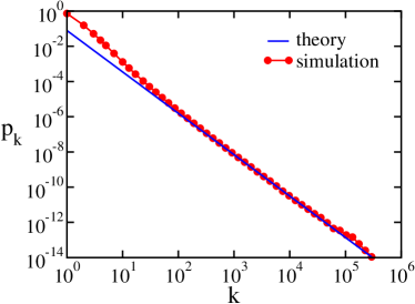
Figure 2: The degree distribution $p_{k}$ versus degree $k$. The simulation results (bullets) are from $10^{2}$ independent realizations with $N=10^{8}$. Also shown is a straight line that corresponds to the theoretical result (1).

The degree distribution is an important quantity that characterizes local properties of networks. For many growing networks, the degree distribution satisfies closed recurrence equations and consequently, this quantity can be determined analytically. It appears impossible to find a closed set of equations that govern the degree distribution for the random ancestor tree. Remarkably, the closed set of equations (9) allows us to obtain the tail of the degree distribution analytically.

The power-law degree of the most connected node (12) already shows that the degree distribution has power-law tail. Let $p_{k}$ be the fraction of all nodes with degree $k$. As announced in (1), this distribution decays algebraically,

$$p_{k}\sim k^{-\gamma}\quad{\rm with}\quad\gamma=\beta+1,$$ (30)

for $k\gg 1$. Indeed, if we substitute $k_{\rm max}\sim N^{1/\beta}$ with $\beta\equiv\beta_{1}$ into the extreme statistics criterion, $N\sum_{k>k_{\rm max}}p_{k}\sim 1$, we obtain (30). Here, we take $\beta=\beta_{1}$ because the exponents $\beta_{n}$ increase monotonically.

Our numerical simulations results are in excellent agreement with the theoretical prediction (1). The simulations are straightforward to implement: with each new node, a target node is selected at random, and then, the attachment node is selected at random from the target node and all of its ancestors. Since the average depth remains finite, the computational cost is proportional to the network size and we can simulate networks as large as $N=10^{8}$. We comment that many real-world networks have power-law degree distributions ab as in (30) with exponent $\gamma$ in the range $2<\gamma<3$. For example, for the Internet at the Autonomous Systems level, as of 2007, the exponent is approximately $\gamma=2.5$, see cskss .

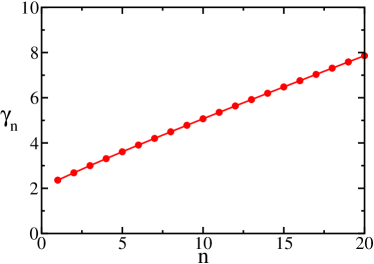
Figure 3: The exponent $\gamma_{n}=1+\beta_{n}$ versus $n$.

Remarkably, the random ancestor tree has a family of degree distributions, each characterized by a distinct nontrivial exponent. The fraction $p_{n,k}$ of $n$th generation nodes with degree $k$ decays algebraically

$$p_{n,k}\sim k^{-\gamma_{n}}\quad{\rm with}\quad\gamma_{n}=\beta_{n}+1.$$ (31)

As in the preferential attachment network, the exponent that characterizes the degree distribution increases with generation bk1 .

From the roots of the transcendental equation $f(\beta_{n})=0$ with $f(\beta_{n})$ given by (26), we find that the exponent $\gamma_{n}$ grows linearly with $n$, that is (figure 3)

$$\gamma_{n}\sim n.$$ (32)

Since $p_{k}=\sum_{n\geq 1}g_{n}p_{n,k}$ and since $g_{n}$ increases with $n$, the dominant contribution to the distribution $p_{k}$ comes from first generation nodes. Hence, $\gamma\equiv\gamma_{1}$. This behavior is in contrast with the preferential attachment network where the behavior at the average generation dominates the degree distribution bk1 .

For completeness, we mention that the in-component distribution mimics the degree distribution. The degree of the in-component of a node is defined as the total number of its descendants. The quantity $h_{\rm tot}$ above is always finite and hence, the total number of descendants of the most connected nodes is proportional to the degree. As consequence, the fraction $I_{s}$ of nodes with in-component degree $s$ decays algebraically, $I_{s}\sim s^{-\gamma}$.

VI Leaves, Stars, and Chains

It is also possible to calculate a few other structural properties of the network including the average number of leaves as well as the probabilities that the network has an extreme structure such as a star or a chain.

Nodes with no incoming links, or equivalently, nodes with degree one are termed leaves. To calculate the total number of leaves, we must first find a more detailed quantity: $L_{n}(N)$, the total number of leaves at the $j$th generation. This quantity evolves as follows

$$\frac{dL_{n}}{dN}=\sum_{i\geq n}\frac{G_{i-1}}{i\,N}-\frac{L_{n}}{(n+1)N}.$$ (33)

Each new node is necessarily a leaf and hence, the gain term is as in (3). The loss term reflects the fact that any new link into a leaf decreases the number of leaves by one.

We assume that the number of leaves in each generation is macroscopic,

$$L_{n}(N)=\ell_{n}N.$$ (34)

By substituting this form into the rate equation (33), we find that leaves constitute a finite fraction of all nodes in each generation, $\ell_{n}=\frac{n+1}{n+2}\,g_{n}$, or equivalently,

$$\ell_{n}=e^{-1}\,\frac{n(n+1)^{2}}{(n+2)!}.$$ (35)

The fraction of leaves grows with depth: 2/3 of all nodes in the first generation are leaves; 3/4 of all nodes in the second generation are leaves; etc. The total number of leaves, $L_{\rm tot}$, is the sum $L_{\rm tot}=\sum_{n\geq 1}L_{n}$ and from (35), we obtain

$$L_{\rm tot}=2e^{-1}N.$$ (36)

As is often the case in complex networks, a large fraction of all nodes have no incoming links.

It is also possible to calculate the likelihood that the tree has one of two extreme topologies: (i) a star where all nodes link to the root, and (ii) a linear chain of length $N$. Let $S_{N}$ be the probability that the tree is a star graph. This probability satisfies the recursion

$$S_{N+1}=S_{N}\left(\frac{1}{N}+\frac{N-1}{2N}\right).$$ (37)

The network is a star graph only if it was previously a star. Furthermore, the factor $1/N$ is the probability that the root is the target node and the factor $(N-1)/(2N)$ is the probability that the target node is any one of the $N-1$ leaves, but the actual link is made to the root. With the boundary condition $S_{1}=S_{2}=1$, the probability $S_{N}$ decays exponentially with the network size,

$$S_{N}=N\,2^{-(N-1)}.$$ (38)

The likelihood that the tree has a chain topology, $C_{N}$, obeys the recursion equation $C_{N+1}=C_{N}/N^{2}$. This recursion reflects that the newest node must always be selected both as the target node and as the attachment node. The probability for this event is $1/N^{2}$. Using the boundary condition $C_{2}=C_{3}=1$, the likelihood of growing a chain decays extremely rapidly,

$$C_{N}=\frac{1}{[(N-1)!]^{2}}.$$ (39)

Therefore, it is far more likely that the random ancestor tree is a star than it is a chain. This is another consequence of the shallow nature of the tree.

VII Conclusions

We introduced a random structure where the genealogy governs the evolution. The random ancestor tree has a remarkably rich structure. The network is very tight with a sharply-decaying distribution of depth. There is a single macroscopic hub that is connected to a finite fraction of all nodes along with multiple highly connected nodes.

The network is strongly stratified because the genealogical structure controls the growth. The most connected node at distance $n$ from the hub has a sub-macroscopic degree that scales as $N^{1/\beta_{n}}$ with system size $N$. Interestingly, the exponents $\beta_{n}$ are generally transcendental numbers. Moreover, the exponents $\beta_{n}$ grow monotonically with $n$, and thus, the connectivity sharply declines with increasing depth. As a consequence, the degree distribution has power-law tail, $p_{k}\sim k^{-\gamma}$ with $\gamma=\beta_{1}+1$ and furthermore, the degree distribution varies strongly with depth.

We obtained all of these features analytically using the total number of descendants of a highly connected node as a function of generation. This quantity obeys a closed set of equations and it allows us to determine many scaling properties including in particular, the exponent that governs the tail of the degree distribution. This theoretical technique has promise in other growing trees problems when the degree distribution does not satisfy closed equations bk ; mgn , especially in situations where the distribution of depth becomes independent of system size asymptotically.

The random ancestor tree includes no control parameters but can be easily generalized by various modifications of the attachment process. More generally, the target node can be selected at a rate that is proportional to the degree and similarly, the attachment node can be determined according to either the generation number or the degree. We envision that such generalizations can be useful for controlling the degree distribution or the number of macroscopic hubs and hence, relevant for modeling complex networks. The most challenging generalization is the theoretical understanding of ancestor networks with cycles.

- (1) D. J. Watts and S. H. Strogatz, Nature 393, 440 (1998).
- (2) R. Albert and A. L. Barabasi, Rev. Mod. Phys. 74, 47 (2002).
- (3) S. N. Dorogovtsev and J. F. F. Mendes, Evolution of Networks: From Biological Nets to the Internet and WWW (Oxford University Press, 2003).
- (4) A. Barrat, M. Barthélemy, A. Vespignani, Dynamical Processes on Complex Networks (Cambridge University Press, New York, 2008).
- (5) G. U. Yule, Phil. Trans. Roy. Soc. B 213, 21 (1925).
- (6) H. A. Simon, Biometrica 42, 425 (1955).
- (7) A. L. Barabasi and R. Albert, Science 286, 509 (1999).
- (8) P. L. Krapivsky, S. Redner, and F. Leyvraz, Phys. Rev. Lett. 85, 4629 (2000).
- (9) S. N. Dorogovtsev, J. F. F. Mendes, and A. N. Samukhin, Phys. Rev. Lett. 85, 4633 (2000).
- (10) J. Kleinberg, R. Kumar, P. Raghavan, S. Rajagopalan, and A. Tomkins, in: Proceedings of the International Conference on Combinatorics and Computing, Lecture Notes in Computer Science, Vol. 1627 (Springer-Verlag, Berlin, 1999).
- (11) P. L. Krapivsky and S. Redner, Phys. Rev. E 63, 066123 (2001).
- (12) R. Lambiotte and M. Ausloos, Europhys. Lett. 77, 58002 (2007).
- (13) P. L. Krapivsky and S. Redner, Phys. Rev. E 71, 036118 (2005).
- (14) S. Wasserman and K. Faust, Social Network Analysis (Cambridge University Press, Cambridge, 1994).
- (15) S. Redner, Eur. Phys. Jour. B 4, 131 (1998).
- (16) M. E. J. Newman, Proc. Natl. Acad. Sci. USA 98, 404 (2001).
- (17) F. Radicchi, S. Fortunato, B. Markines, and A. Vespignani, Phys. Rev. E 80, 056103 (2009).
- (18) H. M. Mahmoud, Evolution of Random Search Trees (John Wiley, New York, 1992).
- (19) P. L. Krapivsky, S. Redner, and E. Ben-Naim, A Kinetic View of Statistical Physics (Cambridge University Press, Cambridge, 2010).
- (20) B. Pittel, Rand. Struct. Algorithms 5, 337 (1994).
- (21) M. E. J. Newman, S. H. Strogatz, and D. J. Watts, Phys. Rev. E 64, 026118 (2001).
- (22) B. Bollobás and O. Riordan, Combinatorica 24, 5 (2004).
- (23) S. N. Dorogovtsev, P. L. Krapivsky, and J. F. F. Mendes, Europhys. Lett. 81, 30004 (2008).
- (24) E. Ben-Naim and P. L. Krapivsky, J. Phys. A 40, 8607 (2007).
- (25) N. Adler and J. Berechman, Transportation Res. A 35, 373 (2001).
- (26) H. Yang and M. G. H. Bel, Transport Rev. 18, 257 (1998).
- (27) M. T. Gastner and M. E. J. Newman, Phys. Rev. E 74, 016117 (2006).
- (28) D. R. Wuellner, S. Roy, and R. M. D’Souza, arXiv:0901.0774.
- (29) P. Krapivsky and D. Krioukov, Phys. Rev. E 78, 026114 (2008).
- (30) The ansatz (12) is consistent with the analysis of Sec. III because vanishes in the thermodynamic limit. The amplitude that appears in (12) varies from realization to realization, but nevertheless, the fractions become deterministic in the thermodynamic limit.
- (31) W. H. Press, S. A. Teukolsky, W. T. Vetterling, and B. P. Flannery, Numerical Recipes, (Cambridge University Press, Cambridge, 1986).
- (32) S. Carmi, S. Havlin, S. Kirkpatrick, Y. Shavitt, and E. Shir, Proc. Natl. Acad. Sci. USA 104, 11150 (2007).
- (33) E. Ben-Naim and P. L. Krapivsky, J. Phys. A 42, 475001 (2009).
- (34) C. Moore, G. Ghosal, and M. E. J. Newman, Phys. Rev. E 74, 036121 (2006).