VLA 1.4GHz observations of the GOODS-North Field: Data Reduction and Analysis

Abstract

We describe deep, new, wide-field radio continuum observations of the Great Observatories Origins Deep Survey – North (GOODS-N) field. The resulting map has a synthesized beamsize of $\sim$1.7″ and an r.m.s. noise level of $\sim$3.9 $\mu$Jy beam^-1 near its center and $\sim$8 $\mu$Jy beam^-1 at 15′  from phase center. We have cataloged 1,230 discrete radio emitters, within a 40′ $\times$ 40′region, above a 5-$\sigma$ detection threshold of $\sim$20 $\mu$Jy at the field center. New techniques, pioneered by Owen & Morrison (2008), have enabled us to achieve a dynamic range of 6800:1 in a field that has significantly strong confusing sources. We compare the 1.4-GHz (20-cm) source counts with those from other published radio surveys. Our differential counts are nearly Euclidean below 100 $\mu$Jy with a median source diameter of $\sim$1.2″. This adds to the evidence presented by Owen & Morrison (2008) that the natural confusion limit may lie near 1 $\mu$Jy. If the Euclidean slope of the counts continues down to the natural confusion limit as an extrapolation of our log N - log S, this indicates that the cutoff must be fairly sharp below 1 $\mu$Jy else the cosmic microwave background temperature would increase above 2.7K at 1.4 GHz.

1 Introduction

The GOODS-N field (Dickinson et al. 2003; Giavalisco et al. 2004) covers $\approx 160$ arcmin² centered on the Hubble Deep Field North (Williams et al. 1996) and is unrivaled in terms of its ancillary data. These include extremely deep Chandra, Hubble Space Telescope and Spitzer observations, deep $UBVRIJHK$ ground-based imaging and $\sim$3,500 spectroscopic redshifts from 8–10-m telescopes. Previous radio observations of this region, however, fell short of complementing this unique dataset.

Table 1: GOODS-North VLA observing log

Observing dates	Integration time (h)	NRAO project code	Configuration
Nov-Dec 1996	42	AR368	A
Feb 2005	28	AM825	B
Aug 2005	7	AM825	C
Dec 2005	2	AM825	D
Feb-Apr 2006	86	AM857	A

Radio emission is a relatively unbiased tracer of star formation and can probe heavily obscured active galactic nuclei (AGN) – objects that are missed by even the deepest X-ray surveys. Radio observations thus allow us to fully exploit the wealth of data taken at X-ray–through–millimeter wavelengths, providing a unique extinction-free probe of galaxy growth and evolution through the detection of starbursts and AGN.

The recent imaging of Owen & Morrison (2008) (OM08) ($\sigma=2.7\,\mu$Jy beam^-1 at 1.4 GHz) have shown that the techniques exist to make radio images that approach the theoretical noise limit. To this end, we have obtained new, deep radio imaging of the GOODS-N field.

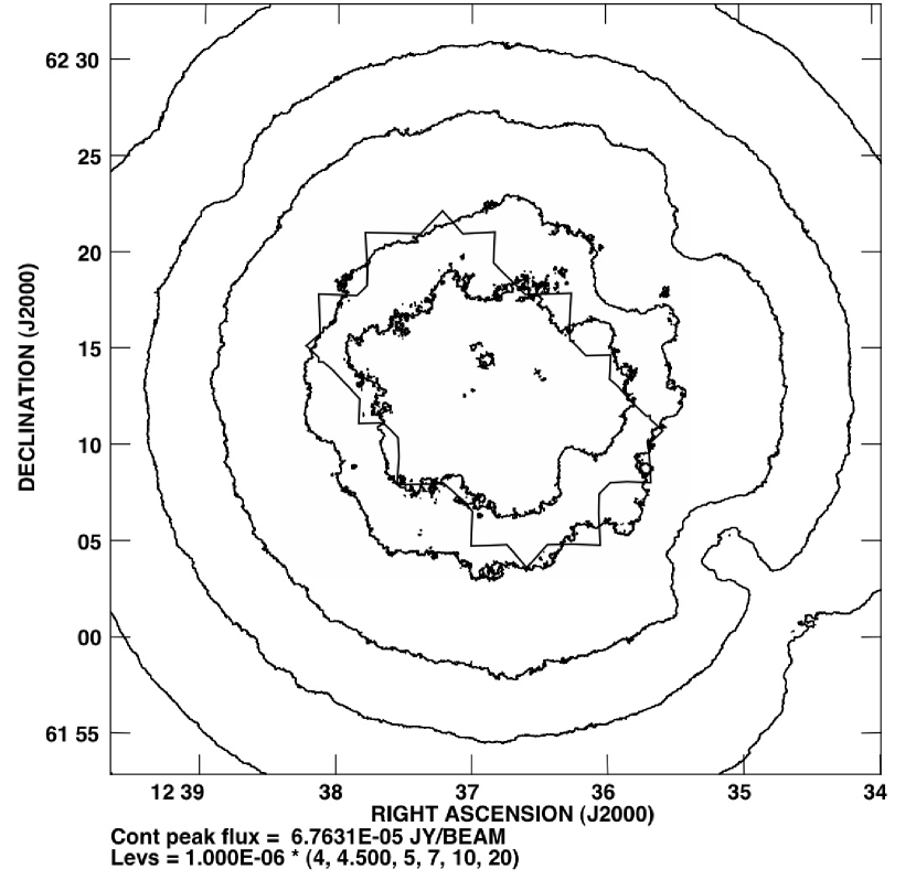
Figure 1: Contours of constant r.m.s. noise after correction for the shape of the primary beam. The GOODS-N area covered by HST/ACS is outlined near the field center, with an average sensitivity of $\sim$3.9 $\mu$Jy beam^-1. At a radius of $\sim$15′ (roughly the half-power point of the primary beam) the r.m.s. sensitivity drops to $\sim$7 $\mu$Jy beam^-1. The strong inward deflection of the 7-$\mu$Jy and 10-$\mu$Jy contours is due to the 265-mJy radio source discussed in §4.4.1.

While GOODS-N was selected to be free from bright sources at optical wavelengths, the field contains several very bright radio sources which place severe limitations on the dynamic range that can be obtained and hence the ultimate sensitivity of the radio map. Before new techniques were developed to deal with this issue, only moderately-deep radio imaging was possible (Richards 2000).

The earliest VLA data in the GOODS-N field were reprocessed using new techniques by Biggs & Ivison (2006) and Morrison et al. (2008), achieving a noise level of 5.7–5.8 $\mu$Jy beam^-1 – a 23-25% improvement on the original map by Richards (2000), and close to the theoretical noise limit when one considers the increase in system temperature at the low elevations permitted during the original observations.

While the reduction of Biggs & Ivison (2006) provided improved access to the $\mu$Jy radio population, even deeper radio imaging is required to properly complement the extremely deep GOODS Spitzer mid-infrared data, as well as forthcoming deep observations at far-infrared and submillimeter wavelengths from Herschel, SCUBA-2, the Large Millimeter Telescope, and other facilities. To this end, we have added 123 hr to the existing data. The reduced full resolution image (beam=1.7″) and its rms map are available online.

The paper is laid out as follows: in §2 we describe the observations and the reduction of the data. In §3 we discuss the cataloging of radio emitters. §4 contains the results and some discussion of the catalog. We present our conclusions in §5.

2 Observations, Reductions, and Cataloging

In 1996 November, Richards (2000) observed a region centered at 12:36:49.4, +62:12:58 (J2000) for a total of 50 hr at 1.4 GHz using the National Radio Astronomy Observatory’s (NRAO’s) VLA in its A configuration. Of this, only 42 hr was considered usable by Richards (2000). Adopting the same position and frequency, we obtained 28 hr of data in the VLA’s B configuration in February–April 2005, 7 hr in C configuration in August 2005, and 2 hr in D configuration in December 2005, and 86 hr in A configuration in 2006 February–April (see Table 1) – for a useful combined total of 165 hr. Observations were done at night to avoid solar interference. We followed the 1:4 scaling of visibility data between the arrays described by OM08. This empirically derived scaling relation provides for more uniform weighting of $uv$ data.

In most regards the new observations were taken using the same parameters as those used in 1996. However, the integration time was changed from 3.33 s to 5 s because of difficulties experienced by the correlator with the shorter integration time (Richards 2000). The data were all obtained using spectral-line mode 4, which yields 7 $\times$ 3.125-MHz channels in each of two intermediate frequencies (IFs), centered at 1,365 and 1,435 MHz, in each of two circular polarizations. The channel width and integration time were compromises chosen to maximize reliability and sensitivity while minimizing bandwidth (radial) and time (tangential) smearing effects, respectively. The upcoming EVLA correlator, WIDAR, will offer much shorter integration times, narrower channels, and greater overall bandwidth.

2.1 Calibration and editing

$\cal AIPS\/$ was used to reduce and analyze all the radio data. The first step was the calculation and corrections of the spectral bandpass shape. This was done in the following manner using the task BPASS. The bright point-source phase calibrator was split from the raw database and phase self-calibration was applied. The self-calibrated data were then used to calculate a bandpass correction and flatten the spectral response across the band for the uncalibrated multi-source database. Standard flux density calibration was applied next, using the Baars flux-density scale with 3C 286 (Baars et al. 1977) as the calibrator. The antenna-based weights for each 5-s integration were also calibrated. The $uv$ data for the target field were split from the database and clipped using the $\cal AIPS\/$ task clip at a level well above the total flux density found in the field to remove any interference prior to the self-calibration process. Only minor interference was encountered during the observations.

2.1.1 UVFIX - Calculating $u,v,$ and $w$

In verifying the astrometry of the A-array data from 1996 and then again in 2006, we found a rotation between the two astrometric frames. The rotational offset was about 1″ at a radial distance of 20′ from the phase center, and is likely the cause of the optical–radio offsets reported regularly over the last decade (e.g. Ivison et al. 2002). The offset problem was traced back to the VLA on-line system (the so-called MODCOMPS) and its calculated $u,v,$ and $w$ terms. This problem was corrected by using the AIPS task UVFIX. This task computes values of $u,v,$ and $w$ using the time index and baseline information recorded during the observations. The $\cal AIPS\/$ task UVFIX was used on all the $uv$ datasets after the initial bandpass and flux calibration.

2.2 Imaging and self-calibration

Bright sources and their sidelobe patterns affect the noise structure and the dynamic range of the final reduced maps if they are not cleaned. Such sources were located using D-configuration data. We imaged to a radius of 8 degrees using a pixel size of 30″. The GOODS-N field was chosen to be free from bright objects at most wavelengths, but not the radio waveband. As a result, bright radio sources limit the dynamic range. We imaged sources as far as 1.5 degrees from the phase center – a total of 56 facets, selected to cover distant, bright sources, plus another five facets within the primary beam to help with the PEELR process which is fully discussed in OM08.

Each facet is constructed from the Fourier transform of the data, phase shifted to its tangent point on the celestial sphere. In all, 98 facets were used. This technique is known as polyhedral imaging (also known as faceting) and is discussed at length by Cornwell & Perley (1992).

One night of A-configuration data was used to lay out 37 facets to cover the primary beam at 1.4 GHz. Each of the 37 facets comprised 1024² pixels, each 0.5″  pixels. The other 56 facets were 512²-pixels in size, again with 0.5²″pixels, centered on the bright, outer sources.

Initial cleaning of the fields with IMAGR revealed faint sources within the 98 facets and tight clean boxes were placed around each one, thus limiting cleaning to real features. Maps were cleaned down to the 1-$\sigma$ noise level to create clean components for use in the self-calibration process. Clean boxes are a vital aspect of this process. They avoid the possibility of cleaning into the noise, which can change the noise structure of a map and result in so-called ‘clean bias’. Failure to use clean boxes can artificially reduce the noise.

This one night of $uv$ data were first self-calibrated in phase only, via the $\cal AIPS\/$ task CALIB, and a new map was made. Self-calibration in amplitude and phase followed. The clean components from this one night were used to construct the fiducial model for the remaining 13 nights of new A-configuration data (AM857 – NRAO project number) as well as the seven nights of 1996 (AR368) A-configuration data. For the four nights of new B-configuration data (AM825), one of the B-configuration datasets were used to provide the clean model for self-calibration. The C- and D-configuration data (AM825) were bootstrapped to the clean model in a similar fashion.

Editing of the $uv$ data was done before and after the self-calibration process using the $\cal AIPS\/$ task TVFLG. After each episode of self-calibration, the clean component model was removed from the $uv$ database using UVSUB. UVPLT was then used to determine the residual amplitude distribution. Any high residual points were deleted with clip, except those on the shortest baselines.

The 165 hr of data resulted in a very large database so we reduced the data volume by exploiting the fact that the A- and B-configuration (programs AM825 and AM857) observations were taken at the same hour angles ($\pm$3.5 hr of transit) over many nights. The smaller hour angle interval helped mitigate the higher system temperature that occurred at lower dish elevations. This is due to the fact that the antenna feeds see the ground at low elevations. The AR368 observing tracks covered $\pm$7.5 hr of transit yielding extended periods of low-elevation observations. The antenna weights were calibrated as part of the standard calibration process minimizing the impact of the more noisy low-elevation data. Finally, STUFFR is used to average data within a small range of u,v (so there is no effect on the image), which was weighted properly. In this way the number of data points used for the imaging were reduced by an order-of-magnitude. This is fully described in OM08.

The five separate datasets were combined into one large $uv$ dataset using DBCON. This was then divided up by hour angle, by Stokes parameter (LL and RR, separately) and by IF, thus yielding eight separate datasets. This last step minimizes the problem of ‘beam squint’ wherein the two circular polarizations have different pointing centers due to the slight off-axis location of the feeds. This, combined with the alt-az telescope mount, causes the effective gain for an off-axis source to vary as a function of time. Moreover, the two IFs are at different frequencies and so yield a different primary beam shapes hence correspondingly different gains for off-axis sources.

Table 2: Sample table of radio sources

Number	R.A. (J2000)	Dec.	SNR	$S_{p}$	$S_{i}$		Size		Upper	Beam
	hms $\pm$ e(s)	d  ′  ″$\pm$ e(″)		($\mu$Jy bm-1)	($\mu$Jy)	Maj	Min	P.A.	(″)	(″)
5	12 34 3.51 0.061	62 14 20.7 0.03	27.6	191.6$\pm$ 6.9	795.9$\pm$ 44.9	2.6	0.7	95	0.0	1.7
9	12 34 8.79 0.164	62 9 20.5 0.10	8.0	51.6$\pm$ 6.5	142.4$\pm$ 19.5	0.0	0.0	0	3.8	1.7
12	12 34 9.23 0.098	61 56 45.5 0.09	44.3	397.0$\pm$ 8.9	2767.1$\pm$ 171.5	7.2	0.0	129	0.0	6.0
13	12 34 9.87 0.238	62 3 57.6 0.12	7.3	57.3$\pm$ 7.9	208.6$\pm$ 30.4	2.8	0.0	89	0.0	1.7
14	12 34 10.61 0.085	62 6 15.8 0.05	18.6	132.1$\pm$ 7.1	564.4$\pm$ 43.5	2.4	0.8	67	0.0	1.7
18	12 34 10.78 0.083	62 2 54.8 0.05	19.2	173.4$\pm$ 9.0	848.0$\pm$ 63.7	2.6	0.5	63	0.0	1.7
22	12 34 11.16 0.029	62 16 17.3 0.02	239.1	1674.0$\pm$ 7.0	7741.0$\pm$ 236.7	8.5	1.6	126	0.0	6.0
23	12 34 11.74 0.003	61 58 32.5 0.00	438.5	4385.0$\pm$ 10.0	27684.0$\pm$ 834.7	1.7	0.6	52	0.0	1.7
35	12 34 16.09 0.071	62 7 22.4 0.05	22.8	127.5$\pm$ 5.6	346.2$\pm$ 18.2	0.0	0.0	0	3.7	3.0
36	12 34 16.17 0.157	62 25 58.8 0.13	8.6	66.1$\pm$ 7.7	284.2$\pm$ 34.6	0.0	0.0	0	3.6	1.7

After self-calibration, some artifacts associated with two bright sources (within the 37 facets that map out the primary beam) remained. A local self-calibration technique in $\cal AIPS\/$ called, PEELR was used to remove these sidelobes. The method is described as follows.

In brief, PEELR subtracts the clean component (CC) model for all facets from the $uv$ data, except for the facet containing the source to be ‘peeled’. Then PEELR self-calibrates using this information (flux) in this facet, writes a new calibration table. Next, PEELR removes the CCs for the chosen field, thereby removing the bright source. The special calibration for this one field aids in the sidelobe correction process. PEELR then goes back to the original calibration tables and adds the CCs back to the $uv$ dataset. Having the $uv$ data in eight separate files allows for a more accurate CC model, enabling more accurate removal of these bright sources.

Full details on this important process can be found in OM08.

2.2.1 Final signal and noise images

The final maps were constructed by combining the 37 central facets made with each of the eight $uv$ datasets, weighting them by $1/\sigma^{2}$, using FLATN. The r.m.s., before correcting for the shape of the primary beam, is $\sim$3.9 $\mu$Jy over a region of 100² pixels. The synthesized beam size is 1.7″ $\times$ 1.6″ with a position angle of $-$5 degrees. The final step was to run $\cal AIPS\/$ task MWFLT which low-pass filters the image with a 101²-pixel kernel to yield a more uniform background.

The $\cal AIPS\/$ task, RMSD, was used to construct a noise image, calculating a histogram based r.m.s. for each pixel using the surrounding pixels within a radius of 100 pixels. A multi-iteration process rejects pixels outside of the $\pm 3\sigma$ range, thereby offering a more robust estimate of the noise. Fig. 1 shows contours of constant noise over the central region, after correcting for the primary beam response.

3 Cataloging

3.1 Angular size effects

The angular size of discrete sources in the image are broadened by three effects: (1) the finite bandwidth of each channel where

$${\rm BWS}\sim\frac{\Delta\nu}{\nu}\times(r),$$ (1)

where $\Delta\nu$ is the fractional bandwidth (i.e. 3.125 MHz) and $r$ is the distance from the phase center; (2) is the finite data sampling rate (estimated at a few percent); (3) and the true angular size of the source. Thus, in order to detect sources above 4.5-sigma, images at 3″and 6″are also needed to detect extended sources–whether truly extended or experimentally extended. OM08 showed that 3″ and 6″ maps are a useful complement to the full-resolution images to recover the full flux of extended sources. The 3″ and 6″ images were made using the $\cal AIPS\/$ task, CONVL.

3.2 Source extraction and cataloging

The $\cal AIPS\/$ task, sad, (‘search and destroy’) was used to generate an initial source catalog. For each resolution, sad was used in ‘signal-to-noise ratio (SNR) mode’ to search for peaks more than 4.5$\times$ the local noise and to correct for radial smearing and primary beam attenuation. This mode uses the noise maps created by RMSD. The final catalog was clipped at $\geq$5$\sigma$.

Residual maps created by sad were searched by eye to find sources missed by the automatic procedure. We made SNR maps from the residual maps, searching for peaks above four. This lower SNR limit was picked because BWS reduces the peak flux of a source. Next, the properties of these sources were measured using $\cal AIPS\/$ task, JMFIT. Sources with SNR greater than 4.5 were retained. Any such sources were added to the catalog for the appropriate resolution.

SAD sources with SNR $\leq$ 5.5 were re-measured by hand using JMFIT – the same task used by sad to determine the source properties. At this low flux limit sad’s automatic detection routine does not always choose the optimal area for analysis. Those pixels within a defined radius (100 pixels) were used to calculate the local noise for each source.

Following OM08, resolved sources were classified on the basis of the best-Gaussian-fit major axis. If the lower limit for this parameter was greater than zero, the source is classed as resolved and the integrated flux was used for the total flux. If lower limit for the major axis was equal to zero (i.e., unresolved) then the peak flux was adopted as the total flux for the source.

There are several extended sources within the central field, as shown in Fig. 3. TVSTAT was used to measure the total flux density of extended sources. The SNRs of extended sources were determined as follows: IMEAN was used to determine the brightest peak and its position was then examined in the noise map; the ratio of these values was adopted as SNR.

Results were then collated following the prescription given in OM08. An additional noise term of 3 % was included for each source to account for calibration errors and uncertainties in the primary beam correction.

4 Results and discussion

4.1 Radio catalog

A sample of the radio catalog is given in Table 2. The complete catalog is available electronically. Column 1 is the source number: source numbers below 10,000 relate to those sources found by sad while those above 10,000 were those found and investigated by hand. Columns 2 and 3 contain the right ascension (R.A.) and the declination (Dec.) in J2000, with the positional error. Column 4 represents the SNR using the ratio of the observed peak flux density and the local noise. In columns 5 we list the peak flux density and its error, in $\mu$Jy beam^-1. Columns 6 contain the total, primary-beam-corrected flux density and uncertainty, in $\mu$Jy. The best-fit deconvolved size (in arcsec) is given in column 7-9. Using our criteria for resolved sources, if a resolved 2-dimensional Gaussian size was the best fit then we give the resulting major and minor fwhm size (in arcsec) along with the position angle (P.A.). If this was not the case then in column 10 we report the major axis upper limit, as estimated by JMFIT or SAD. If the source is resolved then we report 0.0″  for the upper limit size. As noted above, very extended sources, as shown in Fig. 3-11, had their positions, sizes, fluxes and errors measured interactively using IMVAL and TVSTAT. The final column reports the resolution of the map that was used for the measurements for that particular source.

Table 3: Source size summary

Radius	Minimum	Maximum	Sources	Upper	Mean	Error	Median	Resolved
(arcmin)	($\mu$Jy)	($\mu$Jy)		limit	(arcsec)	(arcsec)	(arcsec)	(%)
5	20	30	32	37	1.2	0.1	1.16	46
5	30	100	49	24	1.8	0.2	1.15	67
10	100	300	34	26	2.3	0.4	1.09	57
20	300	1000	48	11	3.4	0.6	1.57	81

4.2 Angular size distribution

As a check on the radio angular size distribution in the GOODS-N field, we have repeated the source size analysis of OM08. The focus of this analysis is to estimate the angular size of the faint radio population. As noted in column 1 of Table 3, we have analyzed the more sensitive inner region ($<$5′) of the radio map for fainter sources while for the brighter sources we expanded our search outward (to 20′) to improve the statistics. Columns 2 and 3 give the flux range and column 4 lists the sources within that size range. Column 5 shows the number of upper limits used with the measured source size distribution in the Kaplan-Meier analysis to derive a robust mean size (column 6) and its associated error (column 7). The median size is reported in column 8 and the percentage of resolved sources used in this analysis is listed in column 9.

The results in Table 3 are consistent with both OM08 and Muxlow et al. (2005), adding to the evidence that the size distribution of the radio population does not continue to decrease below 100 $\mu$Jy and that the median size of such faint emitters is around 1″.

Table 4: Differential normalized source counts for GOODS-N

$S_{\rm l}$	$S_{\rm h}$	$S_{\rm ave}$	No.	$S^{2.5}dN/dS$
($\mu$Jy)	($\mu$Jy)	($\mu$Jy)	#	(Jy1.5 sr-1)
28.0	40.0	34.0	185	7.37$\pm$0.70
40.0	55.0	46.7	187	7.45$\pm$0.89
55.0	90.0	71.1	274	6.67$\pm$0.70
90.0	150.0	113.1	150	7.39$\pm$1.31
150.0	300.0	199.8	107	5.29$\pm$1.11
300.0	1,500.0	557.3	65	6.02$\pm$1.79
1,500.0	60,000.0	5,260.5	17	5.56$\pm$1.68

4.3 Log $N$–Log $S$

We have determined the differential normalized sources counts from our radio catalog using the code and analysis techniques described in detail by OM08. The results are tabulated in Table 4. The relative point-source sensitivity as a function of the distance from the field center for the three resolutions can be seen in figure 4 of OM08. Their figure 5 also shows the relative sensitivity as a function of source size. To summarize, multiple effects can make the source list incomplete, even at rather large SNR. The sensitivity for resolved sources is thus a function of both beam size and distance from the phase center. These effects include (i) primary beam attenuation, (ii) reduction of peak flux due to BWS, (iii) finite time-average smearing and (iv) resolution bias. Sources with integrated fluxes near the survey limit, if extended, will have peak sources below the limit.

As seen in Table 3, the median source size is similar to that of the synthesized beam ($\sim$1.7″). To correct for the effects of this, we adopt the OM08 size distribution, which is based on the properties of sources at higher SNR.

4.4 Comparison to previous surveys

4.4.1 Dynamic range

As described by Biggs & Ivison (2006), and seen in their figure 2, the brightest GOODS-N radio source within the primary beam of the VLA is near 12:34:52, $+$62:02:35. With a primary-beam-corrected total flux of 263 mJy and a peak flux of $\sim$86 mJy beam^-1, it is bright sources like this one (see Fig. 10 upper right) that can limit the dynamic range in an image. This is because there is a limit to how well we can clean these bright sources – a limit determined by how well we can characterize the bandpass, the pointing, the antenna-based gains, and many other parameters. As a result of the imperfect cleaning, residual flux spills into the image from the sidelobes of bright sources. Peak flux density, in Jy beam^-1, is therefore a key quantity when determining the suitability of a field for deep radio imaging, where the ‘beam^-1’ indicates a dependence on resolution.

The reduction by Richards (2000) yielded an image with a dynamic range of $\sim 2,800:1$, with $\sigma=7.5\,\mu$Jy. This was due in part to the fact that self-calibration was not applied to the $uv$ data. Self-calibration and newly developed techniques allowed Biggs & Ivison (2006) to create a more sensitive map, with $\sigma=5.8\,\mu$Jy and a dynamic range of $\sim 4,400:1$. Our reduction, which includes a large quantity of new data (in all VLA configurations) , reaches $\sigma=3.9\,\mu$Jy beam^-1 and a dynamic range of $\sim 6,800:1$.

The $\sim$140-hr VLA observation by Owen & Morrison (2008) – in 1046+59, a field deliberately chosen to be free of strong radio sources – has $\sigma=2.7\,\mu$Jy, which is close to the theoretical noise limit, yet the dynamic range is only $\sim 2,500:1$ because of the paucity of bright radio emitters.

4.4.2 Log $N$–log $S$

Fig. 2 shows our differential source counts below 1 mJy, compared to other deep, 1.4-GHz continuum surveys. Our source counts agree with those for the 1046+59 field where the same methodology was employed for cataloging and for determining log $N$–log $S$: use of multi-resolution maps to build a master source catalog, and the adoption of the same source size distribution.

Above 100 $\mu$Jy our new survey agrees with the counts presented by Biggs & Ivison (2006). Below 100 $\mu$Jy, the counts in the new survey flatten out while those of Biggs & Ivison (2006) began to turn down. This is a well-known issue in deep radio surveys. The difference can be related to a number of complications:

1. We believe that one of the main problems arises from the Gaussian fit not always being the best approach to estimate source properties. Indeed, the intrinsic shape of the sources gets badly affected due to bandwidth and time delay smearing. We have found evidence that flux densities are underestimated systematically after sources have been convolved to lower resolutions – flux densities are larger in the convolved maps. Also, a particular uncertainty comes from the assumption that in unresolved sources we consider the peak flux density as an estimate of the total flux density. These problems clearly suggest the necessity for a more robust source extraction method in radio observations. Another, smaller uncertainties coming from the ‘clean bias’ and ‘flux boosting’ are not expected to be important due to the tight clean boxes we used, and the high 5-$\sigma$ threshold in the source extraction, respectively.

2. A knowledge for the intrinsic radio source size distribution is essential when estimating the number of sources missed by our imaging approach. Muxlow et al. (2005) use high-resolution MERLIN and A-configuration VLA data to tackle this problem, but they miss a non negligible number of low-surface-brightness sources, as is indicated clearly by cross-matching the catalog with lower resolution observations using the WSRT. We believe the combination of VLA data in its A, B, C, and D configurations followed by a source extraction performed in convolved images is essential for detecting these low surface brightness sources ($>$ 4″). A simple source extraction using SAD in the original non-convolved image misses a considerable number of sources as we show in this work. We find that our survey is in good agreement with OM08, so given by the similar treatment, we have adopted their source size distribution for number count estimations.

3. Finally, the source extraction based on a SNR criterion highly depends on reliable estimates of noise as a function of position in the map and the efficiency for detection. Monte-Carlo simulations for the source extraction method (e.g. inserting randomly placed sources in the map and then doing a random search to extract them) are typically used for these purposes. Nevertheless, given our detailed source extraction and our constant examination of residual maps, we believe that our number counts do not suffer significantly from incompleteness down to a threshold of 5$\sigma$. This is why we prefer to perform theoretical corrections, as explained in OM08, rather than a simple Monte-Carlo approach as was in Ibar et al. (2009).

Figure 2: Log $N$–log $S$ for corrected differential source counts below 1 mJy at 1.4 GHz. HDF Biggs, Lockman Hole and ELAIS N2 are from Biggs & Ivison (2006) and SSA 13 is from Fomalont et al. (2006). The 1046+59 data are from Owen & Morrison (2008).

4.4.3 Log $N$–log $S$ Euclidean nature below 100 $\mu$Jy

It is expected that the Cosmic microwave background (CMB) temperature would increase above 2.7K at 1.4 GHz if the counts do not turn over at some flux density below where we have reached. (e.g. Gervasi et al. 2008). The Log $N$–log $S$ results from both the OM08 and the current work suggest that if the Euclidean nature of the counts continue down to the natural confusion as an extrapolation of our log N - log S, this suggests that the cutoff must be fairly sharp below 1 $\mu$Jy.

5 Conclusions

We have presented a deep, new, high-resolution radio image of the GOODS-N field and a catalog containing 1,230 secure radio sources in the central 40′ $\times$ 40′ region. The image reaches an r.m.s. of $\sim$3.9 $\mu$Jy beam^-1 in the best central region. It is thus one of the deepest 1.4-GHz radio surveys ever undertaken, well matched to the excellent Spitzer, Hubble Space Telescope and Chandra data in GOODS-N, and to the upcoming Herschel, SCUBA-2, and the Large Millimeter Telescope imaging at 100–850 $\mu$m and $\sim$1.1-4mm, respectively, providing an unbiased probe of star formation out to $z\sim 3$ and a means to test the calibration of other star-formation rate indicators.

Our analysis of the source size distribution and the counts provide further evidence that the faint 1.4-GHz emitters have a median angular size of $\sim$1.2″, that log $N$–log $S$ remains flat below 100 $\mu$Jy, and that the natural confusion limit at 1.4 GHz must be near 1 $\mu$Jy – a prediction that can be tested in the coming years using the Expanded VLA (EVLA) and e-MERLIN.

Figure 3: Extended sources in the GOODS-N field. Contour levels are listed on the figure and the synthesized beam (FWHM) is illustrated at the bottom left. Several of the sources displayed here might be extended due to band-width smearing issues. The quasi-periodic artifacts are due to uncorrectable correlator errors. In practice, this pattern is not the same for every channel and thus cannot properly be remove from the images by CLEAN deconvolution.

Figure 4: Cont…

Figure 5: Cont…

Figure 6: Cont…

Figure 7: Cont…

Figure 8: Cont…

Figure 9: Cont…

Figure 10: Brightest source in the HDF is in the upper right. Undeconvolvable sidelobes around this source are clearly visible and point to the phase center.

Figure 11: Cont…

References

- Baars et al. (1977) Baars, J. W. M., Genzel, R., Pauliny-Toth, I. I. K., & Witzel, A. 1977, A&A, 61, 99
- Biggs & Ivison (2006) Biggs, A. D. & Ivison, R. J. 2006, MNRAS, 371, 963
- Cornwell & Perley (1992) Cornwell, T. J. & Perley, R. A. 1992, A&A, 261, 353
- Dickinson et al. (2003) Dickinson, M., Papovich, C., Ferguson, H. C., & Budavári, T. 2003, ApJ, 587, 25
- Feigelson & Nelson (1985) Feigelson, E. D. & Nelson, P. I. 1985, ApJ, 293, 192
- Fomalont et al. (2006) Fomalont, E. B., Kellermann, K. I., Cowie, L. L., Capak, P., Barger, A. J., Partridge, R. B., Windhorst, R. A., & Richards, E. A. 2006, ApJS, 167, 103
- Gervasi et al. (2008) Gervasi, M., Tartari, A., Zannoni, M., Boella, G., & Sironi, G. 2008, ApJ, 682, 223
- Giavalisco et al. (2004) Giavalisco, M., Dickinson, M., Ferguson, H. C., Ravindranath, S., Kretchmer, C., Moustakas, L. A., Madau, P., Fall, S. M., Gardner, J. P., Livio, M., Papovich, C., Renzini, A., Spinrad, H., Stern, D., & Riess, A. 2004, ApJ, 600, L103
- Ibar et al. (2009) Ibar, E., Ivison, R. J., Biggs, A. D., Lal, D. V., Best, P. N., & Green, D. A. 2009, MNRAS, 397, 281
- Ivison et al. (2002) Ivison, R. J., Greve, T. R., Smail, I., Dunlop, J. S., Roche, N. D., Scott, S. E., Page, M. J., Stevens, J. A., Almaini, O., Blain, A. W., Willott, C. J., Fox, M. J., Gilbank, D. G., Serjeant, S., & Hughes, D. H. 2002, MNRAS, 337, 1
- Morrison et al. (2008) Morrison, G., Dickinson, M., Owen, F., Daddi, E., Chary, R., Bauer, F., Mobasher, B., MacDonald, E., Koekemoer, A., & Pope, A. 2008, in Astronomical Society of the Pacific Conference Series, Vol. 381, Infrared Diagnostics of Galaxy Evolution, ed. R.-R. Chary, H. I. Teplitz, & K. Sheth, 376
- Muxlow et al. (2005) Muxlow, T. W. B., Richards, A. M. S., Garrington, S. T., Wilkinson, P. N., Anderson, B., Richards, E. A., Axon, D. J., Fomalont, E. B., Kellermann, K. I., Partridge, R. B., & Windhorst, R. A. 2005, MNRAS, 358, 1159
- Owen & Morrison (2008) Owen, F. N. & Morrison, G. E. 2008, AJ, 136, 1889
- Richards (2000) Richards, E. A. 2000, ApJ, 533, 611
- Williams et al. (1996) Williams, R. E., Blacker, B., Dickinson, M., Dixon, W. V. D., Ferguson, H. C., Fruchter, A. S., Giavalisco, M., Gilliland, R. L., Heyer, I., Katsanis, R., Levay, Z., Lucas, R. A., McElroy, D. B., Petro, L., Postman, M., Adorf, H.-M., & Hook, R. 1996, AJ, 112, 1335