Non-Gaussian halo assembly bias
Abstract
The strong dependence of the large-scale dark matter halo bias on the (local) non-Gaussianity parameter, , offers a promising avenue towards constraining primordial non-Gaussianity with large-scale structure surveys. In this paper, we present the first detection of the dependence of the non-Gaussian halo bias on halo formation history using -body simulations. We also present an analytic derivation of the expected signal based on the extended Press-Schechter formalism. In excellent agreement with our analytic prediction, we find that the halo formation history-dependent contribution to the non-Gaussian halo bias (which we call non-Gaussian halo assembly bias) can be factorized in a form approximately independent of redshift and halo mass. The correction to the non-Gaussian halo bias due to the halo formation history can be as large as 100%, with a suppression of the signal for recently formed halos and enhancement for old halos. This could in principle be a problem for realistic galaxy surveys if observational selection effects were to pick galaxies occupying only recently formed halos. Current semi-analytic galaxy formation models, for example, imply an enhancement in the expected signal of and for galaxies at selected by stellar mass and star formation rate, respectively.
1 Institute for Sciences of the Cosmos (ICC), University of Barcelona & IEEC, Barcelona 08028, Spain
2 ICREA (Institució Catalana de Recerca i Estudis Avançats)
3 Max Planck Institute for Astrophysics, P.O. Box 1317, D 85741 Garching, Germany
4 Dipartimento di Fisica “G. Galilei”, Università degli Studi di Padova, via Marzolo 8, I-35131 Padova, Italy
5 INFN, Sezione di Padova, via Marzolo 8, I-35131 Padova, Italy
6 Dipartimento di Astronomia, Università di Bologna, Via Ranzani 1, I-40127 Bologna, Italy
7 INFN, Sezione di Bologna, Viale Berti Pichat 6/2, I-40127 Bologna, Italy
1 Introduction
Placing constraints on deviations from Gaussian primordial fluctuations offers the possibility to test inflationary models [1, 2] and probes aspects of inflation (namely the interactions of the inflaton) that are difficult to probe by other means.
In this paper we focus on the so-called local non-Gaussianity, which describes inflation-motivated departures from Gaussian initial conditions and is parameterized by [3, 4, 5, 6]:
| (1) |
Here denotes a Gaussian field and denotes Bardeen’s gauge-invariant potential, which on sub-Hubble scales reduces to the usual Newtonian peculiar gravitational potential, up to a minus sign. The parameter is the amplitude of the non-Gaussian correction; since and current observational limits restrict [7, 8], we are considering corrections of order .
Recently, Refs. [9, 10] showed that primordial non-Gaussianity affects the clustering of dark matter halos (i.e., density extrema), inducing a scale-dependent bias for halos on large scales. The strong scale-dependence of halo bias () predicted for non-Gaussianity of the local type [9] can provide constraints on competitive with those available from the Cosmic Microwave Background [9, 11, 12]. Analytic estimates of the amplitude of the scale-dependent bias show good agreement with results from -body simulations [9, 13, 14, 15].
Slosar et al. (2008) [7] argue that the amplitude of the non-Gaussian halo bias should depend on the halo merger history. Motivated by the idea that quasar activity is triggered by recent mergers, they estimate the amplitude of the non-Gaussian halo bias for recent mergers. In this paper we extend their reasoning to a more general dependence on the halo merger history through the halo formation redshift . We compare this analysis with the dependence of the non-Gaussian halo bias on halo merger history detected in the -body simulations of Grossi et al. (2009) [13]. By comparison with the halo merger history dependence of the halo occupation distribution of certain galaxies in semi-analytic models of galaxy formation, we estimate the possible impact of these results on predictions for the amplitude of the non-Gaussian bias in upcoming large scale structure surveys.
This paper is organized as follows. In Section 2 we first revisit the extended Press Schechter non-Gaussian halo merger bias derivation of Ref. [7] and then generalize it to arbitrary halo formation redshifts. In Section 3 we detect the effect in -body simulations and show the agreement with the analytic description, including the simple halo mass and redshift dependence predicted by the model. We explore the consequences for practical determination of in Section 4 and we conclude in Section 5. The appendix presents our methodology for fitting our simulation results for the amplitude of the non-Gaussian halo bias mode by mode, i.e. without computing a binned power spectrum.
2 Theory
It has been shown [16] that for non-Gaussianity of the local type considered here, the bispectrum is dominated by the so-called squeezed configurations, triangles where one wavevector length is much smaller than the other two. In other words, local non-Gaussianity introduces strong coupling between large and small scales. It is this coupling that alters halo clustering on large scales (and the halo mass function). In the peak-background split framework, for Gaussian initial conditions, the short-wavelength modes of the density field are responsible for halo collapse and virialization, while the long wavelength ones modulate halo counts. The Lagrange bias of halos of mass at redshift relates their number density (in Lagrange coordinates) to the long wavelength matter overdensity field at redshift :
| (2) |
Upon rearranging this equation, the large scale Lagrange halo bias for halos of mass arising from Gaussian initial conditions is related to the halo number density as
| (3) |
because in the Gaussian case the effect of modulating the density field by a long wavelength mode in some volume of the Universe can be rexpressed simply as an additive change in the effective critical density for collapse in that region. In the presence of mode coupling due to primordial non-Gaussianity, large-scale modes affect the statistical properties of small-scale modes (and vice-versa). For special types of non-Gaussianity (i.e. the local case) it is possible to generalize the Gaussian peak-background split derivation of halo clustering to non-Gaussian initial conditions. This was done in Slosar et al. (2008) [7], which we now summarize.
2.1 Review of Slosar et al. (2008) theoretical results
Slosar et al. (2008) [7] re-cast previous results on non-Gaussian halo bias [9, 10, 17] by instead using a peak-background split of the Gaussian field in Equation 1, where long and short wavelength modes are independent:
| (4) |
The long wavelength density and potential fluctuations are related by the Poisson equation, which can be expressed in Fourier space using with
| (5) |
where is the transfer function and is the linear growth function normalized to in the matter-dominated epoch. That is, is the growth suppression due to non-zero , for which and in a concordance cosmology. We note here that while in this paper refers to the potential in the matter dominated epoch, other authors (e.g., Ref. [13]) have chosen to work with normalized at , the “LSS convention.” The gravitational potential depends on redshift in a non Einstein-de Sitter universe: . We can see from Equation 1 that also depends on this choice, so that . Throughout this section, refers to .
The effect of the non-Gaussianity described by Equation 1 (and its induced mode coupling) is to modulate the amplitude of small-scale density fluctuations with the long wavelength potential fluctuations. This can be viewed as a change in the local value of , , due to :
| (6) |
In this picture, the Lagrangian halo bias becomes
| (7) |
The final expression for the non-Gaussian scale-dependent component of the halo bias on large scale is
| (8) |
where we have dropped the “local” label. That is, under the assumptions of [7], the non-Gaussian scale-dependent halo bias can be predicted from determination of the dependence on of the mass function of the desired objects in cosmologies with Gaussian initial conditions. In particular, to determine for halos of mass that have undergone a recent merger, they write
| (9) |
where is the progenitor mass for a halo of mass that has undergone a recent merger, and is the probability that a halo of mass at has a recent progenitor of mass . For a universal mass function, the first term evaluates to (or [13]). Using the extended Press-Schechter (ePS) formalism, the second term evaluates to -1 (independent of ), in good agreement with the dependence of merger rates on found in -body simulations during the matter-dominated epoch [7]. Ref. [18] finds that in the ePS formalism, the Gaussian halo bias is independent of its formation history. While “halo assembly bias” is the subject of a lot of current theoretical effort (e.g.,[19, 20] and references therein) it appears to be substantial only at the lowest halo masses. -body simulations show that the dependence of halo bias on secondary paremeters is relatively small for the massive halos on very large scales of interest in this work [21, 22, 23, 24, 20, 25]. In particular, Ref. [24] find that for , the 20% youngest halos have a 10% larger Gaussian halo bias than the 20% older halos. Here we concentrate instead on the formation history dependence of the non-Gaussian correction to the halo bias, which, as we show below, is much larger.
2.2 General dependence of on using ePS
In the formalism of ePS, we can easily generalize the results of [7] to express the dependence of on the halo formation history, which we define by the “formation redshift” . In the original formulation of ePS [26], is the redshift at which the halo contains half of its current mass; on the other hand Ref. [27] suggests that, at least for the observational properties of clusters, this should rather be defined as , with . In this section we leave as a free parameter. We can therefore write explicitly in terms of the halo mass observed at redshift with formation redshift , and fraction of the halo mass at , .
| (10) |
Here is the conditional mass function – the probability that a halo with mass at has a mass at an earlier redshift between and . With the same approximations as in Sec 2.5.2 of [26], but generalizing to arbitrary fraction defining the epoch of formation, an analytic expression for the probability distribution of formation redshifts can be derived as follows. We start by defining the amplitude of fluctuations in the linear density field evolved to , as usual:
| (11) |
where is the Fourier transform of a top-hat filter with radius , denotes the matter background density at , and is the linear matter power spectrum at . The second equality makes explicit how we define the in Equation 10 that we differentiate with respect to. That is, defines the amplitude of , while the mass dependence is held fixed. Following Ref [26] we also introduce the quantity
| (12) |
At fixed final halo mass at , the probability that the halo formed between and is simply expressed in terms of :
| (13) |
where (with ) is the critical overdensity for collapse at redshift and denotes the complementary error function. The halo mass, redshift, and dependencies of are absorbed into the variable . To compute the second term in Equation 10, we must differentiate the formation redshift probability distribution at fixed halo mass with respect to :
| (14) |
Therefore, the ePS formalism predicts that the amplitude of the merger history dependent contribution to depends on , , and only through a single variable, . Note that Equation 14 approaches in the limit of large . In Section 3, we test Equation 14 explicitly by dividing our simulated halo sample into bins in . Correspondingly, we must average Equation 14 over the same bins. To reduce the impact of known discrepancies between the ePS prediction for and those measured in -body simulations (e.g., [28]), we express the ePS predictions in terms of the fraction of halos with the lowest or highest values of . For the lowest, we set and solve for such that
| (15) |
For the highest values of , we set and we solve similarly for . The final expression for the mean value of Equation 14 in the range [, ] as a function of halo fraction is
| (16) | |||
One may worry that the expression for the conditional probability (Equation 13) was derived within the Press-Schecter [29] framework: an approximation yielding an expression for the halo mass function which does not reproduce well N-body simulation results especially at small and big masses and which has been significantly improved (e.g., [30, 31]). Unfortunately there is no analytical expression for the conditional probability in the context of these improvements. However, van den Bosch et al. [28] found relatively good agreement between Equation 13 and their -body simulation results, though for the massive halos of interest in this work, the simulated halos formed somewhat earlier than Equation 13 predicts. Moreover, here we are only interested in how changes as is varied; we therefore expect ePS to fare better in this respect. We will show in section that the ePS approach adopted here is a remarkably good description of the dependence of on as measured from N-body simulations.
3 Simulation Results
We use the Grossi et al. (2009) [13] set of 5 simulations (, or equivalently, ), where all simulations use the same initial condition field in Equation 1 to suppress cosmic variance. These simulations have Mpc and particle mass . We generate halo merger trees at with the SUBFIND code [32], based on simulation outputs at (0, 0.137, 0.283, 0.441, 0.613, 0.804, 1.017, 1.258, 1.535, 1.857, 2.236, 2.688, 3.235, 3.907, 4.749, 5.822). To define a halo’s formation redshift , we interpolate between the progenitor masses at the available redshifts.
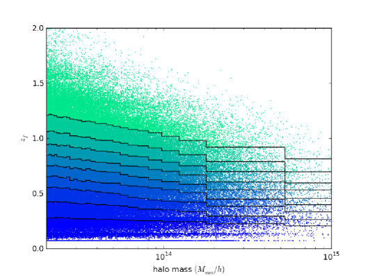
The first term in Equation 10 is proportional to the Gaussian Lagrange halo bias , which depends on halo mass. To separate the dependence of on halo formation redshift from its dependence on halo mass, we create -dependent subsamples of the full mass-limited halo sample at fixed observed redshift that match the halo mass function of the full sample. To do this, we sort the halos by mass, and form groups of halos closest in mass. We sort these halos by , or equivalently by (since the halo mass is nearly constant in the halo subsample). The highest and lowest fraction of these halos enter the -dependent subsamples that by design have matching mass functions. The full sample has at , while we use throughout the main text; in the Appendix we demonstrate that our results are unchanged if is used instead. Figure 1 illustrates the sample selection scheme more clearly, where we plot each halo in our , sample in the two dimensional space -, with the formation in this case defined by for . Note the relatively mild trend that the average decreases with , and also the large spread in at fixed . At each small halo mass bin defined by halos, we divide the sample into 10 bins based on , and the bins from different mass bins are combined to produce halo samples with matching mass functions but different formation redshift distributions. The result is 10 distinct samples represented by the color bands in Figure 1. To increase the signal to noise ratio of our measurements, we do not present non-Gaussian halo bias measurements for the 10 disjoint samples represented in Figure 1, but instead present results for cumulative samples defined by the 9 lines which each divide two colors in the figure. That is, samples labelled as contain either the three lowest or three highest color bands in the figure; the black lines divide the different samples.
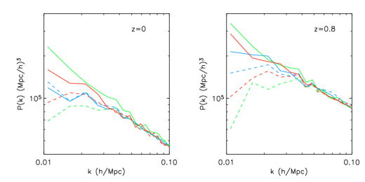
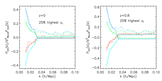
Figure 2 illustrates the signal we quantify in this section. We plot the halo-halo power spectrum for halos with at (left panel) and (right panel) for two subsamples of the parent sample with the 25% highest (blue) and lowest (green) formation redshifts for , selected as described in the previous paragraph. For reference we plot a random subsample of the halo population with the same number density as the -dependent subsamples in red. This should have approximately the same noise properties as the other two samples, but reflects the clustering properties of the full halo population. Dashed lines are for and solid lines are for . In the region of the spectrum where is important (restricted to Mpc in our analysis), the power spectrum is noisy but appears to depend on . Because the spectra show good agreement at higher where is small, our scheme to match the first term in Equation 10 between samples is successful, and the difference between the spectra at small can be attributed to the second (-dependent) term in Equation 10, rather than the term proportional to the Gaussian Lagrange bias .
We assume the following relation between halo () and dark matter () individual Eulerian density modes observed at redshift , in order to fit for the amplitude of the non-Gaussian halo bias, :
| (17) |
Here represents the Eulerian scale-independent contribution to the halo bias (first term in Equation 7). describes the amplitude of the non-Gaussian halo bias, and Equation 10 predicts that is the logarithmic derivative of the Gaussian mass function of the halo sample with respect to , i.e., should be given by . We assume the noise to be Poissonian. For the results presented in this section, we first use the simulation to determine the scale-independent halo bias for each mass, redshift, and -dependent halo subsample while holding . We then assume the and dependence in Equation 17, and fit the four simulations with non-zero for a single number, , for each halo subsample. This accounts for any small dependence of on in the Gaussian case. In the Appendix we present further details of this fitting procedure and compare this approach with a more conservative one, where separate values of are fit simultaneously for each when fitting for . An advantage over previous approaches is that our fit is performed mode by mode for the 366 available modes, rather than to a power spectrum where an effective value of must be chosen for each bin; this choice seemed to impact the results of Ref. [14]. Note that in the model given by Equation 17, , so our measurement error is smallest at where there are the most halos above our fixed mass limit available from our simulations.
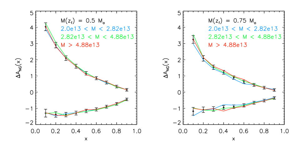
Equation 16 predicts that, when written as a function of the variable , the -dependent fractional contribution to is independent of both halo mass and observed redshift ; we will check these predictions explicitly later in this section. We begin with a mass-limited halo sample at each snapshot redshift available from our simulations and measure the amplitude of its non-Gaussian bias term, . To quantify the dependence of on , we measure :
| (18) |
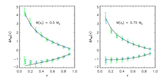
where is the fraction of halos with the highest (lowest) formation redshifts entering the () subsamples at each . In Figure 3 we plot after performing an error-weighted average over all values between and for two definitions of the halo formation redshift, and . Note that is positive, while is negative for both values of . Conservatively, we show the errors from the sample only, since the halo samples at different redshifts will be correlated. Moreover, note that for two values of , , the first subsample is contained in the second. Therefore, the error bars at different are highly correlated as well.
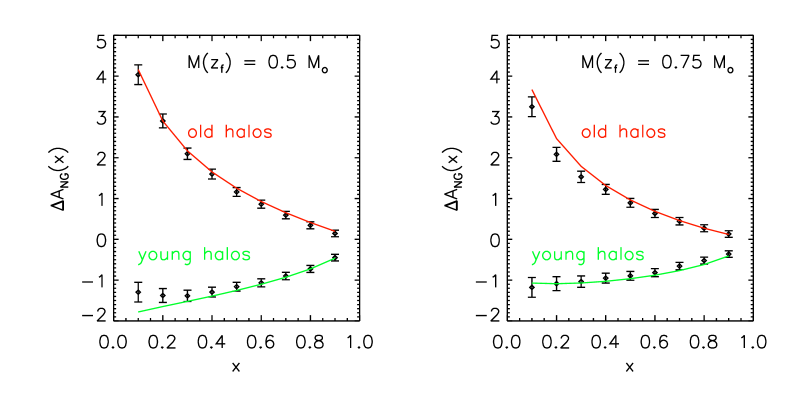
The agreement with the ePS prediction given by Equation 16 is excellent for both the low (green curve) and high (red curve) subsamples. Note that the ePS prediction is:
| (19) |
For the finite binning used in the simulations, the plotted theory line uses Equation 16.
The essential features of the non-Gaussian halo assembly bias we quantify here are:
-
•
The left panel of Figure 4 shows how the relative importance of the first and second term in Equation 10 evolves with redshift, for our mass-limited halo sample; the amplitude of the -dependent contribution is potentially large compared to the first term in Equation 10, . For instance, if we split the , halo sample in two as a function of (i.e., ), the predictions differ from the mean () by . That is, the more recently formed halos have a factor of smaller expected signal than the full halo sample (and with opposite sign: ), while the older halos have a factor of larger signal than the full halo sample ().
-
•
The effect is asymmetric between old and young halos. Even if the tracer population excludes only the 10% oldest halos, the value of for the remaining 90% of the halos differs from the full sample by ; at , this amounts to a change of .
- •
Finally, we generate the closest possible sample to recent major mergers available from our simulations at , where the errors on are smallest. We sort the halo sample not on but on the first progenitor’s mass at the previous snapshot output, (1.7 Gyr earlier). For (i.e., for the 40% of halos with the lowest progenitor masses) we find a consistent with , the ePS prediction derived in Slosar et al. 2008 [7], and the limit of our ePS predictions for large values of .

4 Implications for upcoming galaxy surveys
Non-Gaussianity constraints achievable from forthcoming and planned surveys using halo bias are very promising [11, 33]; these forecasts are obtained using the mean non-Gaussian halo bias relation and therefore assume that these surveys will select galaxies that provide a fair sample of the underlying dark matter halo population in the suitable mass range. However, if the survey selection were to preferentially select galaxies occupying dark matter halos with lower than the mean or were to miss e.g., the 10% of dark matter halos with the highest , this, if unaccounted for, would introduce a significant bias in the measured parameter. As shown in Section 3, in principle, for some extreme cases, this bias could be as large as 40-100% of the (mean) signal.
As alarming as this may seem, it is important to bear in mind that the results of the previous section only affect the predictions of for galaxy redshift surveys if the probability of a halo of hosting a galaxy in the survey sample depends on the formation history of the halo, at fixed halo mass . Within the halo-model framework [34], the standard implementation of the halo occupation distribution approach describes the bias of specific galaxy types with respect to the underlying dark matter by assuming that the probability for a halo to host a galaxy depends only on the halo mass. While for many galaxy types the impact of secondary parameters appears small (e.g., [35, 36, 37] and references therein), there are some indications of halo-assembly bias and evidence for secondary parameters [38, 39, 40]. Semi-analytic models of galaxy formation are dependent on the entire dark-matter halo-merger history and can, in principle, include the full dependence of galaxy properties on secondary parameters. Ref. [41] assessed the impact of Gaussian halo assembly bias for Millenium simulation galaxy samples with two different magnitude cuts, and found changes to the Gaussian bias of . However, this change was not explained by the addition of any simple secondary parameter, like or halo concentration. Therefore, by considering in what follows, we may be underestimating the possible signal from other properties of halo formation that correlate more closely with galaxy properties.
In this section we use galaxies selected from the Bertone et al. (2007) [42] semi-analytic galaxy–formation model implemented on the Millenium simulation halo merger trees [32]. In order to estimate the order of magnitude of this effect, we consider realistic but simply selected galaxy populations relevant to upcoming galaxy surveys, and ask whether these galaxies occupy dark matter halos with specific formation histories, in such a way to introduce a marked non-Gaussian halo assembly bias contribution. Note that the same procedure can be followed to study the impact of halo assembly bias on galaxy clustering in Gaussian initial conditions; in fact, in both cases, we only need to quantify how different the formation redshift distribution of the halo population hosting the selected galaxies is from the full halo population, for a given halo mass (or small around ).
The procedure in the context of a mock galaxy sample embedded in an -body simulation is as follows:
-
•
Select a galaxy sample (e.g., based on observational selection criteria) and identify their host dark matter halos (host halo sample).
-
•
Identify the host dark matter halos’ mass range and select the full dark matter halo sample in that mass range (full halo sample). The halos containing the galaxy sample are a subset of this set.
-
•
Measure the formation-dependent quantity of interest, such as , for the full halo sample.
- •
-
•
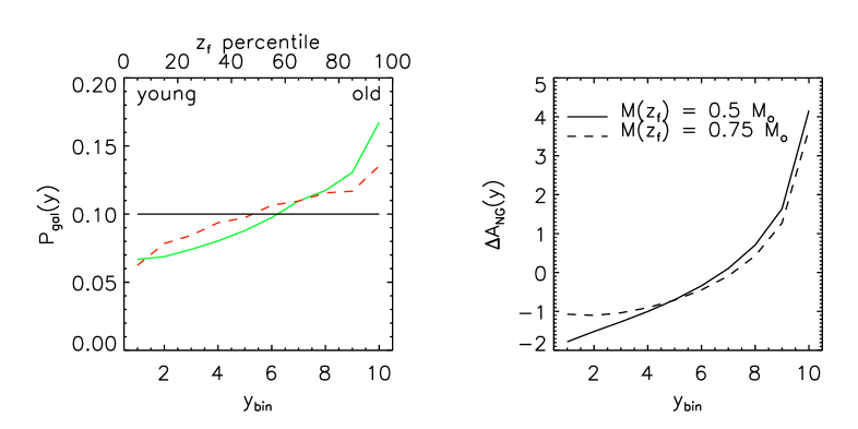
Determine how the halos containing the galaxy sample occupy these 10 bins, summarized by ; here we use to denote the bin number or transversal band in Figure 1. corresponds to halos with 10% lowest for each mass bin and the corresponds to halos with the 10% highest for each mass bin. If galaxies were hosted in a random sample of the full halos, would be a constant. Any deviation from a constant indicates a correlation between the galaxy selection and the host halo formation history. We have chosen the normalization such that .
-
•
Determine the halo assembly bias correction factor. For our application this is :
(20) To evaluate , in practice we break the halos into 10 bins as shown in Figure 1 and sum the expected signal, , over the fraction of galaxies in these discrete bins, . We compute using Equation 16. For this application we are considering disjoint halo subsamples rather than the cumulative bins considered in Figure 3. In the right panel of Figure 6 we show the theory curves for 10 disjoint bins, where we have used () to define in the solid (dashed) curve.
If for some sample galaxies is not negligible compared to , then the effect of non-Gaussian assembly bias cannot be ignored. In particular recall that for recently formed halos, can even cancel out , erasing any non-Gaussian signature, if present.
BigBOSS [43] plans to select luminous red galaxies out to and emission-line galaxies at higher redshift; other proposed surveys (e.g., Euclid [44]) will also target emission-line galaxies out to . Emission-line galaxies are thought to have high star formation rates, possibly triggered by mergers. Should galaxy mergers trace the host dark matter halo mergers, this selection effect could greatly reduce the expected signal for a given value of . Another large future survey suitable for this study is LSST; LSST will select all galaxies above a given magnitude cut, and thus its selection criterion should be less correlated to the host halos accretion history than the other two surveys.
As an example, we consider two distinct galaxy samples from Ref. [42] semi-analytic catalogs at , one selected on large stellar mass () and the other on large star formation rate (), where both samples are chosen to have number densities of , i.e., in the right ballpark for a BAO-focused survey. for these samples is shown by the solid green and red dashed lines in Figure 6 for stellar mass and star formation rate selected samples, respectively; the figure is normalized such that corresponds to a uniform sampling of the underlying halo distribution. For both samples, galaxies occupy halos across the distribution of , but with a preference for halos that formed early (high ), though the trend is stronger with stellar mass. Using Eq. 20, this preference translates to for the stellar mass selected sample, while their Gaussian bias is , as measured from their power spectrum on large scales. For the star formation rate-selected sample, , while their bias is . Since , accounting for the non-Gaussian assembly bias amounts to a boost of the expected scale-dependent halo bias of 23% and 48%, respectively. Results for these galaxy samples are summarized in Table 1.
| Non-Gaussian assembly bias in the Bertone et al. (2007) mock galaxy catalogs | |||||
| selection criteria | % change | ||||
| 0.51 | 2.3 | 2.2 | 23% | ||
| yr | 0.24 | 1.3 | 0.51 | 48% | |
5 Conclusions
We have demonstrated that the impact of assembly bias on the amplitude of the non-Gaussian halo bias can be quite strong. We have expanded the arguments in Slosar et al. (2008) [7] using extended Press-Schechter theory to express non-Gaussian assembly bias in terms of halo formation redshift for arbitrary , where is the redshift at which a halo has accreted a fraction of its final mass. This theory predicts that halo subsamples containing a fraction of the earliest (latest) forming halos (compared with other halos with the same mass) have a non-Gaussian halo bias that differs from the full parent halo sample by a fractional correction dependent only on ; when using this variable, the non-Gaussian assembly bias correction is independent of halo mass and redshift. The -body simulations of Grossi et al. (2009) [13] are in good agreement with these ePS predictions.
The implications of these results for galaxy redshift surveys are extremely uncertain. If the commonly adopted assumption that the probability of a halo hosting a particular type of galaxy only depends on the halo mass, then there will be no non-Gaussian halo assembly bias contribution to the galaxy sample’s non-Gaussian bias. However, in principle, galaxy formation depends on the entire history of host dark matter halos to some degree, and semi-analytic models of galaxy formation attempt to account for this dependence. In Section 4, we found that a relatively mild preference for early-forming halos for both stellar mass and star formation rate selected samples translates into an increase in the expected non-Gaussian galaxy bias of compared with the average signal expected from the samples’ Gaussian bias values. This result is particularly counter-intuitive for star-forming galaxies, since star formation is triggered by galaxy mergers in these models. One should bear in mind that a galaxy merger does not necessarily correspond to a major merger of the host dark matter halo, and that it is reasonable to expect some time-lag between the dark matter halo merger and the merger of the galaxies populating them. Furthermore, we caution that we have not been extensive in our exploration of galaxy sample selection space, or precise enough to make predictions for upcoming experiments. There may be certain populations for which this effect may be much larger or much smaller. On the other hand, it is possible that in an analysis aimed at constraining , one may be able to weight galaxies by some color or spectral property in order to enhance the non-Gaussian signal in the survey. More work is needed to further quantify the impact of such an approach on the recovered constraints on from realistic surveys.
Acknowledgements
We thank the anonymous referee for going beyond the call of duty and independently cross-checking our results. Non-Gaussian -body simulations have been performed on the IBM-SP5 at CINECA (Consorzio Interuniversitario del Nord-Est per il Calcolo Automatico), Bologna, with CPU time assigned under an INAF-CINECA grant, and on the IBM-SP4 machine at the “Rechenzentrum der Max-Planck-Gesellschaft” at the Max-Planck Institut für Plasmaphysik with CPU time assigned to the “Max-Planck-Institut für Astrophysik” and at the “Leibniz-Rechenzentrum” with CPU time assinged to the Project “h0073.” The Millennium Simulation databases used in this paper and the web application providing online access to them were constructed as part of the activities of the German Astrophysical Virtual Observatory. BR is supported by OISE/0530095. LV acknowledges support of FP7-PEOPLE-2007-4-3-IRG n. 20182, FP7-IDEAS Phys.LSS 240117 and MICCIN grant AYA 2008-03531. LV thanks for hospitality IPMU, where the last stages of this work were carried out. KD acknowledges the support of the DFG Priority Program 1177. This research has been partially supported by ASI Contract No. I/016/07/0 COFIS and ASI/INAF Agreement I/072/09/0 for the Planck LFI Activity of Phase E2. LM acknowledges contracts Euclid-Dune I/064/08/0, ASI-INAF I/023/05/0, and ASI INAF I/088/06/0.
References
References
- [1] N. Bartolo, E. Komatsu, S. Matarrese, and A. Riotto, Non-Gaussianity from inflation: theory and observations, Physics Reports 402 (Nov., 2004) 103–266, [astro-ph/0406398].
- [2] E. Komatsu, N. Afshordi, N. Bartolo, D. Baumann, J. R. Bond, E. I. Buchbinder, C. T. Byrnes, X. Chen, D. J. H. Chung, A. Cooray, P. Creminelli, N. Dalal, O. Dore, R. Easther, A. V. Frolov, J. Khoury, W. H. Kinney, L. Kofman, K. Koyama, L. Leblond, J. Lehners, J. E. Lidsey, M. Liguori, E. A. Lim, A. Linde, D. H. Lyth, J. Maldacena, S. Matarrese, L. McAllister, P. McDonald, S. Mukohyama, B. Ovrut, H. V. Peiris, A. Riotto, Y. Rodrigues, M. Sasaki, R. Scoccimarro, D. Seery, A. Sefusatti, K. M. Smith, A. A. Starobinsky, P. J. Steinhardt, F. Takahashi, M. Tegmark, A. J. Tolley, L. Verde, B. D. Wandelt, D. Wands, S. Weinberg, M. Wyman, A. P. S. Yadav, and M. Zaldarriaga, Non-Gaussianity as a Probe of the Physics of the Primordial Universe and the Astrophysics of the Low Redshift Universe, in AGB Stars and Related Phenomenastro2010: The Astronomy and Astrophysics Decadal Survey, vol. 2010 of Astronomy, No. 158, 2009.
- [3] D. S. Salopek and J. R. Bond, Nonlinear evolution of long-wavelength metric fluctuations in inflationary models, Phys. Rev. D 42 (Dec., 1990) 3936–3962.
- [4] A. Gangui, F. Lucchin, S. Matarrese, and S. Mollerach, The three-point correlation function of the cosmic microwave background in inflationary models, ApJ 430 (Aug., 1994) 447–457.
- [5] L. Verde, L. Wang, A. F. Heavens, and M. Kamionkowski, Large-scale structure, the cosmic microwave background and primordial non-Gaussianity, MNRAS 313 (Mar., 2000) 141–147, [astro-ph/9906301].
- [6] E. Komatsu and D. N. Spergel, Acoustic signatures in the primary microwave background bispectrum, Phys. Rev. D 63 (Mar., 2001) 63002.
- [7] A. Slosar, C. Hirata, U. Seljak, S. Ho, and N. Padmanabhan, Constraints on local primordial non-Gaussianity from large scale structure, Journal of Cosmology and Astro-Particle Physics 8 (Aug., 2008) 31, [arXiv:0805.3580].
- [8] E. Komatsu, K. M. Smith, J. Dunkley, C. L. Bennett, B. Gold, G. Hinshaw, N. Jarosik, D. Larson, M. R. Nolta, L. Page, D. N. Spergel, M. Halpern, R. S. Hill, A. Kogut, M. Limon, S. S. Meyer, N. Odegard, G. S. Tucker, J. L. Weiland, E. Wollack, and E. L. Wright, Seven-Year Wilkinson Microwave Anisotropy Probe (WMAP) Observations: Cosmological Interpretation, ArXiv e-prints (Jan., 2010) [arXiv:1001.4538].
- [9] N. Dalal, O. Doré, D. Huterer, and A. Shirokov, Imprints of primordial non-Gaussianities on large-scale structure: Scale-dependent bias and abundance of virialized objects, Phys. Rev. D 77 (June, 2008) 123514, [arXiv:0710.4560].
- [10] S. Matarrese and L. Verde, The Effect of Primordial Non-Gaussianity on Halo Bias, ApJ Lett. 677 (Apr., 2008) L77–L80, [arXiv:0801.4826].
- [11] C. Carbone, L. Verde, and S. Matarrese, Non-Gaussian Halo Bias and Future Galaxy Surveys, ApJ Lett. 684 (Sept., 2008) L1–L4, [arXiv:0806.1950].
- [12] L. Verde and S. Matarrese, Detectability of the Effect of Inflationary Non-Gaussianity on Halo Bias, ApJ Lett. 706 (Nov., 2009) L91–L95, [arXiv:0909.3224].
- [13] M. Grossi, L. Verde, C. Carbone, K. Dolag, E. Branchini, F. Iannuzzi, S. Matarrese, and L. Moscardini, Large-scale non-Gaussian mass function and halo bias: tests on N-body simulations, MNRAS 398 (Sept., 2009) 321–332, [arXiv:0902.2013].
- [14] A. Pillepich, C. Porciani, and O. Hahn, Halo mass function and scale-dependent bias from N-body simulations with non-Gaussian initial conditions, MNRAS 402 (Feb., 2010) 191–206, [arXiv:0811.4176].
- [15] V. Desjacques, U. Seljak, and I. T. Iliev, Scale-dependent bias induced by local non-Gaussianity: a comparison to N-body simulatio ns, MNRAS 396 (June, 2009) 85–96, [arXiv:0811.2748].
- [16] D. Babich, P. Creminelli, and M. Zaldarriaga, The shape of non-Gaussianities, Journal of Cosmology and Astro-Particle Physics 8 (Aug., 2004) 9, [astro-ph/0405356].
- [17] N. Afshordi and A. J. Tolley, Primordial non-Gaussianity, statistics of collapsed objects, and the integrated Sachs-W olfe effect, Phys. Rev. D 78 (Dec., 2008) 123507, [arXiv:0806.1046].
- [18] S. R. Furlanetto and M. Kamionkowski, Pair correlations and merger bias, MNRAS 366 (Feb., 2006) 529–536, [astro-ph/0507650].
- [19] L. Gao and S. D. M. White, Assembly bias in the clustering of dark matter haloes, MNRAS 377 (Apr., 2007) L5–L9, [astro-ph/0611921].
- [20] N. Dalal, M. White, J. R. Bond, and A. Shirokov, Halo Assembly Bias in Hierarchical Structure Formation, ApJ 687 (Nov., 2008) 12–21, [arXiv:0803.3453].
- [21] L. Gao, V. Springel, and S. D. M. White, The age dependence of halo clustering, MNRAS 363 (Oct., 2005) L66–L70, [astro-ph/0506510].
- [22] R. H. Wechsler, A. R. Zentner, J. S. Bullock, A. V. Kravtsov, and B. Allgood, The Dependence of Halo Clustering on Halo Formation History, Concentration, and Occupation, ApJ 652 (Nov., 2006) 71–84, [astro-ph/0512416].
- [23] A. R. Wetzel, J. D. Cohn, M. White, D. E. Holz, and M. S. Warren, The Clustering of Massive Halos, ApJ 656 (Feb., 2007) 139–147, [astro-ph/0606699].
- [24] Y. P. Jing, Y. Suto, and H. J. Mo, The Dependence of Dark Halo Clustering on Formation Epoch and Concentration Parameter, ApJ 657 (Mar., 2007) 664–668, [astro-ph/0610099].
- [25] A. Faltenbacher and S. D. M. White, Assembly Bias and the Dynamical Structure of Dark Matter Halos, ApJ 708 (Jan., 2010) 469–473, [arXiv:0909.4302].
- [26] C. Lacey and S. Cole, Merger rates in hierarchical models of galaxy formation, MNRAS 262 (June, 1993) 627–649.
- [27] P. T. P. Viana and A. R. Liddle, The cluster abundance in flat and open cosmologies, MNRAS 281 (July, 1996) 323, [astro-ph/9511007].
- [28] F. C. van den Bosch, The universal mass accretion history of cold dark matter haloes, MNRAS 331 (Mar., 2002) 98–110, [astro-ph/0105158].
- [29] W. H. Press and P. Schechter, Formation of Galaxies and Clusters of Galaxies by Self-Similar Gravitational Condensation, ApJ 187 (Feb., 1974) 425–438.
- [30] R. K. Sheth, H. J. Mo, and G. Tormen, Ellipsoidal collapse and an improved model for the number and spatial distribution of dark matter haloes, MNRAS 323 (May, 2001) 1–12, [astro-ph/9907024].
- [31] A. Jenkins, C. S. Frenk, S. D. M. White, J. M. Colberg, S. Cole, A. E. Evrard, H. M. P. Couchman, and N. Yoshida, The mass function of dark matter haloes, MNRAS 321 (Feb., 2001) 372–384.
- [32] V. Springel, S. D. M. White, A. Jenkins, C. S. Frenk, N. Yoshida, L. Gao, J. Navarro, R. Thacker, D. Croton, J. Helly, J. A. Peacock, S. Cole, P. Thomas, H. Couchman, A. Evrard, J. Colberg, and F. Pearce, Simulations of the formation, evolution and clustering of galaxies and quasars, Nature 435 (June, 2005) 629–636, [astro-ph/0504097].
- [33] C. Carbone, O. Mena, and L. Verde, Cosmological Parameters Degeneracies and Non-Gaussian Halo Bias, ArXiv e-prints (Mar., 2010) [arXiv:1003.0456].
- [34] A. Cooray and R. Sheth, Halo models of large scale structure, Physics Reports 372 (Dec., 2002) 1–129.
- [35] R. Skibba, R. K. Sheth, A. J. Connolly, and R. Scranton, The luminosity-weighted or ‘marked’ correlation function, MNRAS 369 (June, 2006) 68–76, [astro-ph/0512463].
- [36] R. A. Skibba and R. K. Sheth, A halo model of galaxy colours and clustering in the Sloan Digital Sky Survey, MNRAS 392 (Jan., 2009) 1080–1091, [arXiv:0805.0310].
- [37] J. L. Tinker, C. Conroy, P. Norberg, S. G. Patiri, D. H. Weinberg, and M. S. Warren, Void Statistics in Large Galaxy Redshift Surveys: Does Halo Occupation of Field Galaxies Depend on Environment?, ApJ 686 (Oct, 2008) 53–71, [arXiv:0707.3445].
- [38] A. Mateus, R. Jimenez, and E. Gaztañaga, The Scale Dependence of Mass Assembly in Galaxies, ApJ Lett. 684 (Sept., 2008) L61–L64, [arXiv:0801.3282].
- [39] M. C. Cooper, C. A. Tremonti, J. A. Newman, and A. I. Zabludoff, The role of environment in the mass-metallicity relation, MNRAS 390 (Oct., 2008) 245–256, [arXiv:0805.0308].
- [40] M. C. Cooper, A. Gallazzi, J. A. Newman, and R. Yan, Galaxy assembly bias on the red sequence, MNRAS 402 (Mar., 2010) 1942–1958, [arXiv:0910.0245].
- [41] D. J. Croton, L. Gao, and S. D. M. White, Halo assembly bias and its effects on galaxy clustering, MNRAS 374 (Feb., 2007) 1303–1309, [astro-ph/0605636].
- [42] S. Bertone, G. De Lucia, and P. A. Thomas, The recycling of gas and metals in galaxy formation: predictions of a dynamical feedback model, MNRAS 379 (Aug., 2007) 1143–1154, [astro-ph/0701407].
- [43] D. J. Schlegel, C. Bebek, H. Heetderks, S. Ho, M. Lampton, M. Levi, N. Mostek, N. Padmanabhan, S. Perlmutter, N. Roe, M. Sholl, G. Smoot, M. White, A. Dey, T. Abraham, B. Jannuzi, D. Joyce, M. Liang, M. Merrill, K. Olsen, and S. Salim, BigBOSS: The Ground-Based Stage IV Dark Energy Experiment, ArXiv e-prints (Apr., 2009) [arXiv:0904.0468].
- [44] R. Laureijs, Euclid Assessment Study Report for the ESA Cosmic Visions, ArXiv e-prints (Dec., 2009) [arXiv:0912.0914].
- [45] R. E. Smith, R. Scoccimarro, and R. K. Sheth, Scale dependence of halo and galaxy bias: Effects in real space, Phys. Rev. D 75 (Mar., 2007) 063512, [astro-ph/0609547].
- [46] U. Seljak, N. Hamaus, and V. Desjacques, How to Suppress the Shot Noise in Galaxy Surveys, Physical Review Letters 103 (Aug., 2009) 091303, [arXiv:0904.2963].
Appendix A Fitting non-Gaussian bias
We wish to construct a to estimate the amplitude of halo assembly-bias in non-Gaussian simulations; in principle this would require knowledge of a 4-point function in the non-Gaussian theory. We begin considering the expected errors in linear theory for Gaussian initial conditions, and linearly biased tracers that Poisson-sample the continuous matter density field. Our model for the relation between the halo density field and the matter density field for each mode is given by Equation 17, and Poisson sampling implies . We will keep the -dependence of the non-Gaussian component of the bias fixed, , and fit for an amplitude of the non-Gaussian component, , and scale-independent component, . Under these assumptions, the variance about the model is
| (21) |
Here the average is over the Poisson noise, and the matter field is considered fixed. For our calculation, we will only consider the real component of . Since the noise is assumed uncorrelated with , the noise associated with only the real component is smaller by a factor of 2 than in Equation 21, which counts both real and imaginary components.
| (22) |
Because there may be a slight dependence of on , we consider two distinct fitting procedures for . In both, we assume the and dependence in Equation 10 and define one and two sigma errors by changes in the value of 1 and 4 in Equation 22, where the sum is performed over the density modes of interest in each different simulation. Following Ref. [13], we limit all fits to modes with Mpc, which after discarding modes with wavenumber and , amounts to 366 modes. We find that for the massive halos considered here, can be substantially smaller than the number of degrees of freedom (see [45, 46] for other recent evidence for sub-Poissonian sampling). Therefore, our error bars may be overestimated.
In the first approach applied in the main text, we first fit the model with to the simulation to determine and its uncertainty for each mass, redshift, and -dependent halo subsample. Next we fit for using the four simulations, assuming that the scale-independent contribution, , is independent of . Therefore we use the measurement in the simulation to marginalize over a common to all values of , integrating over the probability distribution derived from the result.
In the second, more conservative approach, we fit our simulation data to a five parameter model: the scale-independent in each non-zero simulation, and a single amplitude for the non-Gaussian signal. Because of the limited range of values over which to fit, the non-Gaussian amplitude can be degenerate with the scale-independent bias in Equation 17. Figure 7 shows an example of this. We first fit the simulation for in the same range we use to fit the non-Gaussian bias (Mpc), holding . To illustrate the non-Gaussian signal, we plot the halo-matter cross power spectrum normalized by for (blue, green, red, light blue). We plot the best fit five parameter model in black for Mpc, and we plot the value of for each value at Mpc. The best fit values of are anti-correlated with the value of in the sample, which could in principle affect the best fit value for . We compare the results of the five and one parameter fits to in Figure 8. The two approaches give consistent results, though the errors are much larger as expected when is fit separately for each value of .
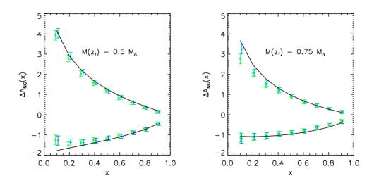
In Section 3 we introduce the parameter , which determines how many halos are grouped together before dividing into subsamples based on . If is too small, one expects to introduce sample variance, in that halos are scattered across boundaries because each set of halos is a finite sampling of the true distribution. However, if is too large, then one will introduce a spurious dependence through the dependence of on halo mass. In Figure 9 we compare values for and , and demonstrate that our results are insensitive to this choice.
