On the solar chromosphere observed at the limb with Hinode

Abstract

Broad-band images in the Ca II H line, from the BFI instrument on the Hinode spacecraft, show emission from spicules emerging from and visible right down to the observed limb. Surprisingly, little absorption of spicule light is seen along their lengths. We present formal solutions to the transfer equation for given (ad-hoc) source functions, including a stratified chromosphere from which spicules emanate. The model parameters are broadly compatible with earlier studies of spicules. The visibility of Ca II spicules down to the limb in Hinode data seems to require that spicule emission be Doppler shifted relative to the stratified atmosphere, either by supersonic turbulent or organized spicular motion. The non-spicule component of the chromosphere is almost invisible in the broad band BFI data, but we predict that it will be clearly visible in high spectral resolution data. Broad band Ca II H limb images give the false impression that the chromosphere is dominated by spicules. Our analysis serves as a reminder that the absence of a signature can be as significant as its presence.

,

1 Introduction

The Hinode spacecraft is a stable platform from which unique high resolution, seeing-free images of the Sun can be acquired (Kosugi et al., 2007). The BFI instrument, fed by the Solar Optical Telescope (SOT) on Hinode (Tsuneta et al., 2008), can observe a 3 Å wide spectral bandpass centered at the H line of Ca II. Over this bandpass, the line forms in both the photosphere in the wings, and chromosphere in the core. Movies of such Ca II images have revealed a remarkably dynamic, spicule-dominated limb. The observed spicules have smaller diameters, higher apparent velocities and smaller lifetimes (de Pontieu et al., 2007) than was previously thought (Beckers, 1968, 1972).

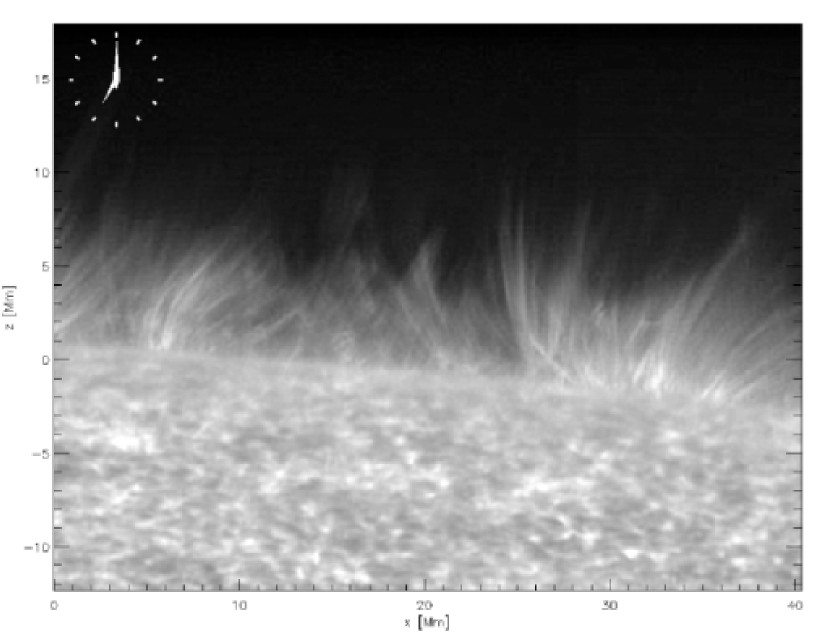
Figure 1: A snapshot from a time series of Ca II images obtained with the 3 Å wide filter of the BFI instrument using the SOT on the Hinode spacecraft. The height scale has been carefully determined, relative to the vertical continuum (5000 Å) optical depth unity, by Bjølseth.

Figure 1 shows a typical snapshot from a series of Ca II BFI images acquired on 7 November 2007, in the northern polar coronal hole. We selected a coronal hole because spicules there are longer than elsewhere, thereby providing a broad background of spicule emission against which a stratified atmosphere might easily be identified. A smooth radial gradient has been divided out of the data to enhance the emission high above the limb. The zero point of the height scale $z=0$ (along $x=0$) corresponds to the standard formation height of the 5000 Å continuum, when observed vertically, as derived by Bjølseth (2008). Henceforth we will refer to heights on this standard scale. Bjølseth found that the Ca II limb lies $0.45\pm 0.034$ Mm above the blue limb. Since the continuum at the limb forms about 0.375 Mm higher than at disk center, (e.g., Athay, 1976), the Ca II limb forms near heights of 0.825 Mm.

Curiously, such limb images show little or no signature of a bulk, stratified chromosphere which, as we discuss below, should have a thickness between 1 and 2 Mm. The BFI instrument’s resolution ($\sim 0\farcs 1$) is ample to resolve structure on scales of 1-2 Mm ($0\farcs 1\equiv 0.0725$ Mm). Yet a striking feature of these images is the continuous emission seen along each spicule all the way down to, and sometimes across, the limb. Where then is the stratified chromosphere, and why are spicules so obviously dominant that one might conclude that the chromosphere itself consists of little more than a collection of spicules? In this paper we explore what these observations imply in terms of the structure of the chromosphere.

2 Simple calculations

The complex dynamic behavior of the Ca II spicules, their unknown origin and other difficulties preclude the possibility of meaningful ab-initio or other detailed modeling efforts. To address the above questions, a far simpler calculation is appropriate. We model the chromosphere as a stratified atmosphere from which spicules emanate. Formal solutions to the transfer equation along rays tangential to the solar limb are performed for prescribed source functions, densities and atomic parameters applicable to the Ca II H line.

Our adopted stratified medium is simply the 1D atmosphere of Gingerich et al. (1971). As suggested by the Hinode BFI observations, this medium does not emit as much as the embedded spicules, so it serves primarily to scatter photons. The exact stratification of the bulk chromosphere is not critical, all that is required is that it span the range of densities from photosphere to corona in $\mathrel{\hbox to0.0pt{\lower 3.5pt\hbox{$\sim$}\hss}\raise 1.5pt\hbox{$<$}}2$ Mm. The mean stratifications of hydrodynamic or MHD models, such as by Carlsson and Stein (1995); Wedemeyer-Böhm et al. (2009), are similar to the stratification used here.

The stratified atmosphere was assigned source functions of $B_{\nu}(T(r))f(r)$ where $T(r)$ is taken from the atmospheric model, as a function of radial distance from Sun center $r$. $B_{\nu}(T)$ is the Planck function at frequency $\nu$ and temperature $T$. The function $f(r)$ mimics well-known non-LTE effects in which source functions fall below their LTE values. Figure 2 shows the source functions used in our calculations.

The spicules were treated statistically, both in their spatial distributions and thermodynamic properties. They were randomly distributed along the boundaries of circular supergranules into 200 small bushes with a common “root”, 8 spicules in each bush. 1600 spicules per supergranule, each with a diameter of 0.1 Mm, leads to a filling factor by area of 0.015, and a total of $2\times 10^{7}$ such spicules on the Sun at any time. (The latter is some 20 times larger than the value derived by Beckers 1972, based upon data of far lower angular resolution than those from the Hinode BFI instrument). These numbers produce synthetic spicule images similar to those from Hinode.

The roots of individual spicules are set at $r_{0}=1.25$ Mm above the continuum photosphere, with a base density $\rho=\rho_{0}=1.4\times 10^{-11}$ g cm^-3. Below the $r_{0}$ there are no spicules in our calculations- the atmosphere is 100% “stratified”. The spicules are modeled simply as longer extensions of the atmosphere from this base. The spicule densities are $\rho(r)=\rho_{0}\,e^{-(r-r_{0})/\ell_{s}}$ with $\ell_{s}=3.5$ Mm for $r>r_{0}$. The scale height $\ell$ was chosen to match intensity scale heights of $\sim 3.5$ Mm found for polar coronal holes by (Bjølseth, 2008), in order to compare calculations with Figure 1. The calculated intensities depend only weakly on the gas densities, because our source functions are fixed and the spicules have optical depths of order $10^{1}$ in the line cores. The assumed spicule properties will be revisited in the Section 4.

Spicule orientations were randomized relative to the local vertical in azimuth, and their source functions specified along each one’s length but randomly varied between spicules. The source functions are not individually known, being determined locally by collisional excitation and scattering of radiation from the bright underlying photosphere. Makita (2003, fig. 12) shows source functions below 4 Mm with black body temperatures near 4300K. Here, each spicule’s base source function was chosen from a randomly distributed sample about a mean of $B_{\nu}(T=4300{\rm K})$ with an arbitrary distribution width one tenth of this. Along each spicule the source function drops with height along with the density. Fig. 2 shows the mean value as a function of height. For the line opacity, all calculations use a calcium logarithmic abundance of 6.3 (where H=12), all calcium is assumed to be in Ca II (a good approximation below the transition region) an absorption oscillator strength of 0.33, a microturbulence of 10 km s^-1 (except where specified below) and a radiatively damped Voigt profile. Standard continuum opacity was added to the line opacity from Allen (1973).

3 Results

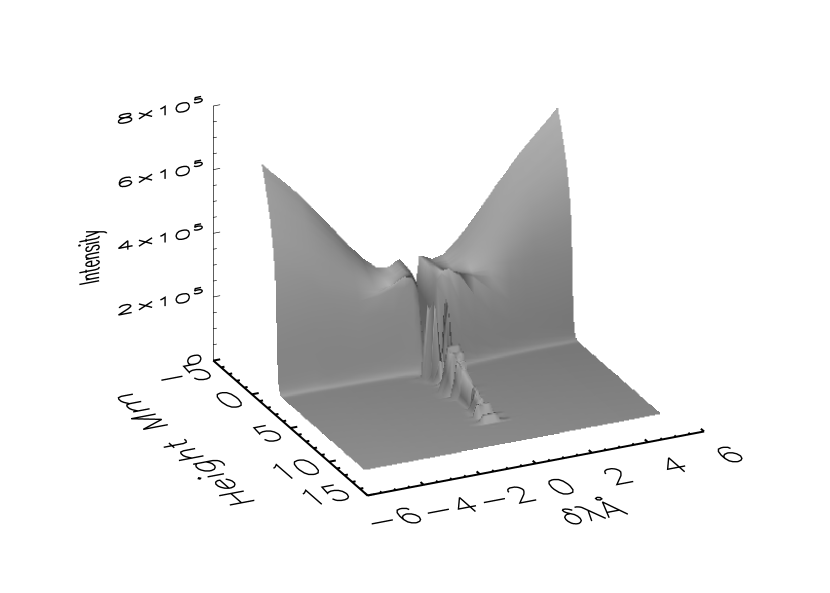
Figure 3: Line profiles computed from a radial slice of the “standard” transfer calculations, simply to demonstrate that the computed spectra are not dissimilar to those observed. The self-reversed core in the photosphere (heights near zero) change to emission in the spicular material at greater heights.

Figure 3 shows intensity profiles of the H line as a function of wavelength and height in a “standard” model. The computed intensities are similar to observations both above and below the limb. The chosen Ca II line parameters produce results not incompatible with typical profiles seen on the disk (Linsky and Avrett, 1970), and with Ca II observations obtained both during and outside eclipses (Beckers, 1968, 1972; Makita, 2003).

Figure 4 shows emergent intensities at various monochromatic wavelengths and integrated over the BFI filter bandpass. In the “standard” calculation (left panels), the spicule line profiles are assumed to be the same as in the stratified atmosphere. The latter leads to absorption at wavelengths within 0.1 Å of line center and below heights of $\sim 2$ Mm. The path lengths and line opacity of the stratified material are sufficient to produce absorption, unless a spicule happens to lie physically closer to the observer. The limb in the simulated BFI data (see the panel labeled “Hinode BFI Ca II”) is close to the $0.875$ Mm value derived observationally by Bjølseth (2008). In the lowest panels, the same radial function was applied to the simulated data as the observations shown in Figure 1, to enhance the visibility of spicule emission over the limb. In the broad BFI bandpass, a significant and observable fraction of spicule emission is absorbed by the stratified atmosphere below 2-3 Mm. This behavior is inconsistent with the appearance of Hinode data.

Real spicules are dynamic, as seen both through linewidths and physical motions (Beckers, 1968, 1972; Makita, 2003; de Pontieu et al., 2007). Therefore we made two further calculations: one using broad spicule emission line profiles, and another using spicule-aligned flows. Both calculations shift the spicule emission outside of the absorption profiles of the stratified atmosphere when the Doppler speeds exceed $\xi\sqrt{\ln\tau_{0}}$, where $\xi$ is the chromospheric microturbulence ($\mathrel{\hbox to0.0pt{\lower 3.5pt\hbox{$\sim$}\hss}\raise 1.5pt\hbox{$<$}}c_{s}$, the sound speed, $c_{s}\sim 7$  km s^-1, e.g., Vernazza et al., 1981), and $\tau_{0}>1$ is the line center optical depth tangential to the limb. For values of $\tau_{0}$ varying between 10 and $10^{10}$ the required shifts are a few times $c_{s}$.

The right hand panels of Figure 4 present calculations including a spicule line broadening microturbulent parameter drawn from a distribution with a mean of 30  km s^-1 and a standard deviation of 10  km s^-1. This supersonic microturbulence is compatible with linewidths measured from eclipse data below about 4 Mm (e.g. Makita, 2003). (In the dynamic calculation, not shown, spicule-aligned outflows were drawn from a distribution with a mean of 120  km s^-1 and a standard deviation of 40  km s^-1.) In this calculation, the spicules can be seen down to and crossing the limb, as observed, and the dark absorption band resulting from the stratified atmospheric absorption is less pronounced. Figure 5 shows intensities in the BFI bandpass averaged along the direction tangential to the limb, normalized to limb values, as a function of height, from the three calculations and from observations. The filter-integrated emission from broad spicule line profiles is larger than from the standard calculation, because the computed individual spicules are optically thick across their axes, at least for heights below 4 Mm.

The differences in the broad dips in intensity between heights of 1 and 2.5 Mm shows our main result- dynamical calculations are needed to avoid such a large dip in BFI Ca II intensities across the limb.

4 Discussion

It seems that the absence of the stratified chromosphere in the images obtained with the Hinode BFI Ca II filter may be explained, at least in part, simply by large Doppler shifts resulting from spicule dynamics. The computations (Figure 4) resemble observations (Figure 1) when spicule emission is Doppler shifted out of the dark core of the H line in the stratified chromosphere.

4.1 From photosphere to corona

The solar atmosphere does not end at the visible photosphere- there must exist material as the upwardly stratified extension of the photosphere. This material must, on average, be highly stratified because quiet Sun coronal pressures are close to 0.1  dyn cm^-2 (e.g. Mariska, 1992), yet photospheric pressures are orders of magnitude higher. The only question of interest here is if this material is expected to be able to scatter the Ca II resonance lines. Even if the chromosphere were in hydrostatic and radiative equilibrium, and hence maximally stratified, almost all of the calcium would be in the Ca II ground state, and the stratified layer would span $\sim 1$ Mm before coronal conditions were reached. In semi-empirical 1D models the transition from photosphere to corona spans 1.5 Mm (measured from temperature minimum to corona, Gingerich et al., 1971; Athay, 1976; Vernazza et al., 1981).

This transition must, on average, be stratified close to hydrostatic equilibrium, because motions observed in spectral lines formed in the photosphere and chromosphere are, statistically speaking, sub-sonic. Indeed one has to look hard to find the on-disk counterparts of the highly supersonic type II spicules (McIntosh and De Pontieu, 2010), for example. More directly observable signatures of the stratified chromospheric medium are found, for example, in the “flash spectrum” seen during eclipses (Makita, 2003, and references therein), or in the upward extension of photospheric wave motions seen on the solar disk. While the observationally-defined “chromospheric extent” inferred by flash spectra exceeds hydrostatic values, it is also compatible with a hydrostatic stratification in the first 1-1.5 Mm. The large extent arises primarily from the data seen high above the limb which are dominated by spicules. These and other issues are reviewed by, e.g., Gibson (1973); Athay (1976); Judge (2006).

4.2 Validity of our results

The ad-hoc parameters in our calculations clearly limit their usefulness. But our essential result- the need to Doppler shift spicule material out of the absorbing stratified chromosphere in order to reproduce qualitatively Hinode Ca II data- is relatively insensitive to such details. The result simply requires spicules to originate close to the base of the chromosphere, and have different source functions and/or opacities from the stratified atmosphere. Given these conditions, and spicule lengths which exceed the thickness of the stratified atmosphere, our result appears robust. Our particular choice of parameters were taken from observed properties discussed by Makita (2003); de Pontieu et al. (2007). For a given density, the opacity in the Ca II H line follows from atomic data, ion abundance, and thermal and non-thermal motions. Average densities of the stratified medium are, as we argued above, approximately in hydrostatic equilibrium. However, our spicule densities and their height dependence were chosen simply to produce computations qualitatively similar to the particular coronal hole data shown in Figure 1.

Physical considerations suggest that $\rho_{0}$ cannot greatly exceed $10^{-11}$ g cm^-3. de Pontieu et al. (2007); McIntosh and De Pontieu (2010) find these spicules to be highly supersonic, $\sim 100$ km s^-1. Such high speeds require magnetic forces in plasma where the sound speed is certainly $\mathrel{\hbox to0.0pt{\lower 3.5pt\hbox{$\sim$}\hss}\raise 1.5pt\hbox{$<$}}10$ km s^-1. While the mechanism driving spicules is not known, the characteristic Alfvén speed $v_{A}$ must exceed 100 km s^-1. Using an upper limit of 1 kG for field strengths in the low chromospheric network (1 kG is characteristic of network photospheric fields), $v_{A}\sim 100$ km s^-1, we find $\rho<10^{-9}$ g cm^-3. But this is an unrealistically large estimate, since chromospheric magnetic fields are weaker due to geometric expansion of network fields, and not all of the local magnetic energy is free to be converted to kinetic energy. Strong network magnetic fields tend also to be largely unipolar, thus only tangential components associated with magnetic shear or with weaker neighboring opposite polarity fields contain the free energy. Adopting field strengths nearer to 0.1 kG, as an order of magnitude estimate, the observed spicule speeds require $\rho\sim 10^{-11}$ g cm^-3, as used above. It is difficult to see how this estimate can be significantly larger.

Spicules in coronal holes are longer, as seen in ground based data (Beckers, 1972) and in Hinode data (de Pontieu et al., 2007; Bjølseth, 2008). Our scale height of 3.5 Mm for coronal hole densities and source functions is twice the value derived for the numbers of spicules observed as a function of height for the Sun in general by Beckers (1972). Bjølseth (2008) shows in her Fig. 4.10 that the Hinode Ca II data of equatorial regions have scale heights closer to 2 Mm. The relationship between the spicules observed by the Hinode BFI instrument and earlier work has not yet been clarified. We simply note that our calculations are not unrealistic parameterizations of the conditions needed to describe radiative transfer in the chromosphere of a coronal hole.

Our computations are not in qualitative disagreement with the 1.5 Mm wide dip in H$\alpha$ line center intensities discovered by Loughhead (1969). The cores of H$\alpha$ and neutral helium lines routinely show a dip in intensity surrounded by a shell of emission (e.g. White, 1963; Loughhead, 1969; Pope and Schoolman, 1975, and much later work). However, dips seen in visible lines of hydrogen and helium may result more from the well-known lack of opacity in the low to mid chromosphere, and extra opacity due to fibrils which appear to over-arch the stratified chromosphere. Resolving the issue would require detailed calculations of H$\alpha$ and He lines with models taking into account the fibril structure and excitation mechanisms populating these excited atomic levels, which are not currently feasible.

Lastly, there remains an interesting discrepancy between the Hinode BFI data and flash spectra, in that the 2 Mm Ca II scale height is twice the median value derived from flash spectra of Ca II lines (Makita, 2003, his table 2, see also our Fig. 5). Importantly we also note that our calculations never remove the off-limb dip entirely, even in the dynamic and broad line calculations, yet at least some of the Hinode BFI images appear to show no hint of a dip.

4.3 Implications

Both observations and simple physical arguments require that spicules be a consequence of some plasma or magnetohydrodynamic processes occurring within the chromosphere. Spicules cannot arise fully fledged from the photosphere for several reasons, not least because photospheric and spicular densities and gas pressures differ by many orders of magnitude.

Our result suggests that the Hinode BFI Ca II images can be used as speedometers in the sense that spicules, when visible down to the limb, must have components that are Doppler shifted supersonically, say by more that say 20  km s^-1. While the limb chromosphere appears in the Hinode BFI Ca II data to be made entirely of spicules, this broad bandpass appears to be almost blind to much of the stratified, inter-spicule chromosphere. The Hinode BFI Ca II filter probably misses populations of the short “type-I” spicules also associated with the magnetic network, whose line widths and Doppler shifts are insufficient to avoid the absorption by the intervening material.

In fact, these Hinode data miss the bulk of the mass of the chromosphere, including the internetwork. Standard chromospheric models give on average 0.03 g cm^-2 as the total chromospheric surface mass density (e.g. Vernazza et al., 1981). The mass density per unit area of the spicules, averaged over the surface, is $\sim\rho\ell f$ where $\rho$, $\ell$ and $f$ are their typical mass density, length and surface filling factor. Using $\rho\sim 1.4\times 10^{-11}$ g cm^-3, $\ell\sim 3.5\times 10^{8}$ cm, $f=0.015$, we find an average mass density of only $7\times 10^{-5}$ g cm^-2. The spicules observed by the Hinode Ca II BFI instrument comprise less than 0.3% of the entire chromospheric mass. The energy flux density needed to support the network chromosphere against radiation losses is estimated to be a few times $10^{7}$ erg cm^-2 s^-1 (Anderson and Athay, 1989). The enthalpy flux density of individual spicules with speeds of 100  km s^-1 is $pv\sim 3\times 10^{7}$ erg cm^-2 s^-1, which is thus comparable. Perhaps then these Hinode spicules are intrinsically related to the chromospheric heating that is observed?

5 Conclusions

Hinode BFI Ca II images obtained at the solar limb are consistent with the presence of the stratified chromosphere when spicular emission is Doppler shifted relative to the stratified material. This can be achieved most naturally using broad and/or Doppler shifted spicule line profiles of magnitudes compatible with observed motions. The picture presented here can be tested directly using very stable spectra at the solar limb, to see for example if the behavior modeled in Figure 4 is qualitatively correct. This is a very challenging observation to make from the ground, but should be possible under conditions of outstandingly good seeing and with modern adaptive optics systems.

The calculations reinforce a commonly known problem regarding broad band spectral imagers: one must be very careful taking care of physical effects such as Doppler motions which are not spectrally resolved by the instrument. BFI Ca II limb observations are largely blind to the bulk of the chromosphere itself. This fact is a sobering reminder that the absence of a signature can be as significant as its presence.

Figure 2: Prescribed source functions used in the calculations. The spicules were treated statistically.

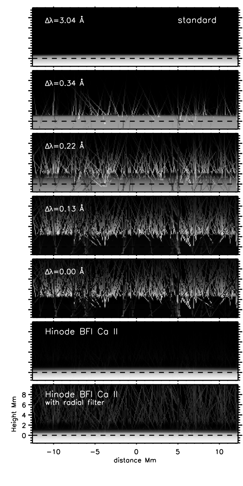
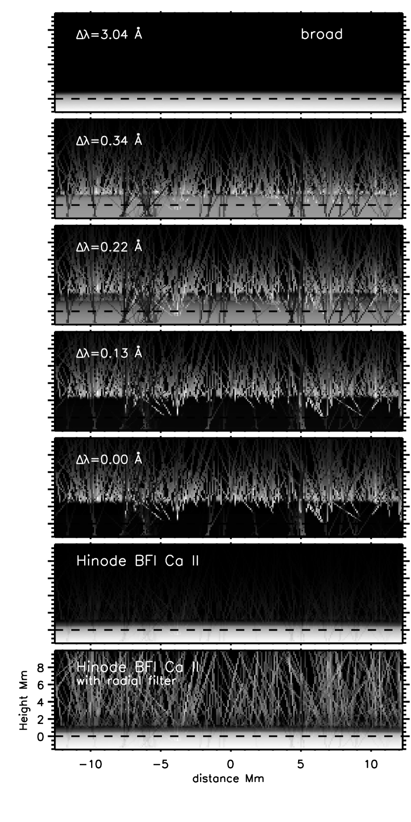
Figure 4: Intensities computed at several monochromatic wavelengths and in the Hinode BFI passband are shown as a function of position along the limb tangential diretion and radial height. The “standard” spicule conditions were applied (left panel), and broad spicular emission lines were computed (right panel).

Figure 5: Average intensities, normalized to the same point within the solar limb, are plotted for observations and for three model calculations. Also shown is the height dependence of the Ca II emission found by Makita (2003) from eclipse flash spectra, the absolute value of which is arbitrary.

References

- Allen (1973) Allen, C. W.: 1973, Astrophysical Quantities, Athlone Press, Univ. London
- Anderson and Athay (1989) Anderson, L. S. and Athay, R. G.: 1989, Astrophys. J. 336, 1089
- Athay (1976) Athay, R. G.: 1976, The Solar Chromosphere and Corona: Quiet Sun, Reidel: Dordrecht
- Beckers (1968) Beckers, J. M.: 1968, Solar Phys. 3, 367
- Beckers (1972) Beckers, J. M.: 1972, Ann. Rev. Astron. Astrophys. 10, 73
- Bjølseth (2008) Bjølseth, S.: 2008, Master’s thesis, Oslo University
- Carlsson and Stein (1995) Carlsson, M. and Stein, R. F.: 1995, Astrophys. J. 440, L29
- de Pontieu et al. (2007) de Pontieu, B., McIntosh, S., Hansteen, V. H., Carlsson, M., Schrijver, C. J., Tarbell, T. D., Title, A. M., Shine, R. A., Suematsu, Y., Tsuneta, S., Katsukawa, Y., Ichimoto, K., Shimizu, T., and Nagata, S.: 2007, Publ. Astron. Soc. Japan 59, 655
- Gibson (1973) Gibson, E. G.: 1973, The quiet sun, NASA SP, Washington: National Aeronautics and Space Administration
- Gingerich et al. (1971) Gingerich, O., Noyes, R. W., Kalkofen, W., and Cuny, Y.: 1971, Solar Phys. 18, 347
- Judge (2006) Judge, P.: 2006, in J. Leibacher, R. F. Stein, and H. Uitenbroek (Eds.), Solar MHD Theory and Observations: A High Spatial Resolution Perspective, Vol. 354 of Astronomical Society of the Pacific Conference Series, 259
- Kosugi et al. (2007) Kosugi, T., Matsuzaki, K., Sakao, T., Shimizu, T., Sone, Y., Tachikawa, S., Hashimoto, T., Minesugi, K., Ohnishi, A., Yamada, T., Tsuneta, S., Hara, H., Ichimoto, K., Suematsu, Y., Shimojo, M., Watanabe, T., Shimada, S., Davis, J. M., Hill, L. D., Owens, J. K., Title, A. M., Culhane, J. L., Harra, L. K., Doschek, G. A., and Golub, L.: 2007, Solar Phys. 243, 3
- Linsky and Avrett (1970) Linsky, J. L. and Avrett, E. H.: 1970, Publ. Astron. Soc. Pac. 82, 169
- Loughhead (1969) Loughhead, R. E.: 1969, Solar Phys. 10, 71
- Makita (2003) Makita, M.: 2003, PNAOJ 7, 1
- Mariska (1992) Mariska, J. T.: 1992, The Solar Transition Region, Cambridge Univ. Press, Cambridge UK
- McIntosh and De Pontieu (2010) McIntosh, S. W. and De Pontieu, B.: 2010, Astrophys. J. Lett. in press
- Pope and Schoolman (1975) Pope, T. and Schoolman, S. A.: 1975, Solar Phys. 42, 47
- Tsuneta et al. (2008) Tsuneta, S., Ichimoto, K., Katsukawa, Y., Nagata, S., Otsubo, M., Shimizu, T., Suematsu, Y., Nakagiri, M., Noguchi, M., Tarbell, T., Title, A., Shine, R., Rosenberg, W., Hoffmann, C., Jurcevich, B., Kushner, G., Levay, M., Lites, B., Elmore, D., Matsushita, T., Kawaguchi, N., Saito, H., Mikami, I., Hill, L. D., and Owens, J. K.: 2008, Solar Phys. 249, 167
- Vernazza et al. (1981) Vernazza, J., Avrett, E., and Loeser, R.: 1981, Astrophys. J. Suppl. Ser. 45, 635
- Wedemeyer-Böhm et al. (2009) Wedemeyer-Böhm, S., Lagg, A., and Nordlund, Å.: 2009, Space Science Reviews 144
- White (1963) White, O. R.: 1963, Astrophys. J. 138, 1316