MRI-driven turbulent transport: the role of dissipation, channel modes and their parasites.

Abstract

Context. In the recent years, MRI-driven turbulent transport has been found to depend in a significant way on fluid viscosity $\nu$ and resistivity $\eta$ through the magnetic Prandtl number $Pm=\nu/\eta$. In particular, the transport decreases with decreasing $Pm$; if persistent at very large Reynolds numbers, this trend may lead to question the role of MRI-turbulence in YSO disks, whose Prandtl number is usually very small.

Aims. In this context, the principle objective of the present investigation is to characterize in a refined way the role of dissipation. Another objective is to characterize the effect of linear (channel modes) and quasi-linear (parasitic modes) physics in the behavior of the transport.

Methods. These objectives are addressed with the help of a number of incompressible numerical simulations. The horizontal extent of the box size has been increased in order to capture all relevant (fastest growing) linear and secondary parasitic unstable modes.

Results. The major results are the following:
i- The increased accuracy in the computation of transport averages shows that the dependence of transport on physical dissipation exhibits two different regimes: for $Pm\lesssim 1$, the transport has a power-law dependence on the magnetic Reynolds number rather than on the Prandtl number; for $Pm>1$, the data are consistent with a primary dependence on $Pm$ for large enough ($\sim 10^{3}$) Reynolds numbers.
ii- The transport-dissipation correlation is not clearly or simply related to variations of the linear modes growth rates.
iii- The existence of the transport-dissipation correlation depends neither on the number of linear modes captured in the simulations, nor on the effect of the parasitic modes on the saturation of the linear modes growth.
iv- The transport is usually not dominated by axisymmetric (channel) modes.

1 Introduction

Disks evolve on time-scales that are orders of magnitudes smaller than expected from microphysical transport processes, and various suggestions have been made over the years to explain this discrepancy. Turbulent transport, in particular, has figured among the leading candidates since the inception of the $\alpha$-disk paradigm, and a number of hydrodynamic and MHD turbulent transport mechanisms have been proposed in the literature.

On the hydrodynamic side, subcritical turbulence (Richard & Zahn 1999 and references therein), if present, is apparently too inefficient (Lesur & Longaretti, 2005; Ji et al., 2006). Convection was up to now found too inefficient and to transport angular momentum in the wrong direction (Cabot, 1996; Stone & Balbus, 1996), but a recent reinvestigation of the problem indicates that this might be an artifact of these simulations being performed too close to the stability threshold (Lesur & Ogilvie, 2010). Two-dimensional weak turbulence driven by small-scale, incoherent gravitational instabilities (density waves) is an option (Gammie, 1996). Alternatively, the baroclinic instability (Klahr & Bodenheimer, 2003) may generate vorticity, and transport through the coupling with density waves, but its conditions of existence are still controversial (Johnson & Gammie, 2006; Petersen et al., 2007), although Lesur & Papaloizou (2010) have probably identified the root of this debate by pointing out the nonlinear nature of the instability; also the resulting vortices would be subject to 3D instabilities (Lesur & Papaloizou, 2009).

Balbus & Hawley (1991) have proposed that the magnetorotational instability (MRI) is a potentially efficient source of turbulent transport in the nonlinear regime, an expectation soon borne out in numerical simulations. This instability provides by now the most extensively studied transport mechanism, through local unstratified (Hawley et al., 1995), stratified (Stone et al., 1996), and global (Hawley, 2000) 3D disk simulations. These initial simulations as well as the numerous ones following them have shown that MRI turbulence is an efficient way to transport angular momentum, in the presence or absence of a mean vertical or toroidal field, with an overall transport efficiency depending on the field configuration and strength. However, the significant role played by microphysical dissipation in the resolutions accessible to date had largely been underestimated (Lesur & Longaretti, 2007; Fromang et al., 2007).

By now, both the field strength and dissipation dependence of the simulated turbulent transport have been studied to some extent (and only in unstratified local shearing box settings for the latter one). The dependence of the Shakura-Sunyaev $\alpha$ parameter has been characterized very early on by Hawley et al. (1995) who showed that momentum transport $\propto\beta^{-1/2}$ both for a net vertical or toroidal field (albeit with very different efficiencies in the two configurations), a scaling further confirmed in later simulations, as summarized in Pessah et al. (2007).

Until recently, the effect of physical viscosity ($\nu$) and resistivity ($\eta$) on the transport had been neglected, under the implicit assumption that these should not matter too much once inertial turbulent scales are resolved in the simulations. However, Lesur & Longaretti (2007) have shown that, in the presence of a mean vertical field, the MRI-driven turbulent transport did exhibit a substantial dependence on the magnetic Prandtl number $Pm=\nu/\eta$, with no clear trends with respect to either viscosity of resistivity alone. Recently, Simon & Hawley (2009) found similar results in shearing boxes with a mean toroidal field instead of a mean vertical one.

When the mean magnetic flux vanishes, the transport behavior is more complex. The initial investigation by Hawley et al. (1996) concluded that the transport was converging to a finite value, but Gardiner & Stone (2005) found that the transport efficiency was dependent on the simulation resolution. More recently, the role of the magnetic Prandtl number $Pm$ has been identified in this setting (Fromang et al., 2007): turbulence exists only for magnetic Prandtl numbers larger than about 2, which requires the explicit inclusion of viscous and resistive terms in the fluid equations for numerical simulations to correctly capture the physics of the problem. The disappearance of turbulence at low $Pm$, as well as the need of large enough amplitudes in the initial conditions at $Pm>2$, indicate that the zero net flux magnetized shearing box is a subcritical system rather than a linearly unstable one (Lesur & Ogilvie, 2008a, b).

Thus it appears that in all configurations explored to date, the magnetic Prandtl number plays a significant role on the existence and/or efficiency of the turbulent transport, at least at the resolutions accessible on present day computers (or equivalently, the accessible Reynolds and magnetic Reynolds numbers). This raises a number of issues.

For one, the exact role played by channel modes and parasitic modes is unclear. Although they exist only when a mean vertical field is present, they are simpler to analyze and their behavior may provide insight into the generic mechanism responsible for saturation of the linear instability. Channel modes are the axisymmetric unstable modes of the MRI (Balbus & Hawley, 1991; Pessah & Chan, 2008), and are often observed both in 2D and 3D simulations with a mean vertical field; their name derives from their vertically layered characteristic channel-like radial flow. They were quickly recognized to be also nonlinear solution of the problem by Goodman & Xu (1994); the same authors found them to be unstable with respect to a secondary instability (parasitic modes). A few recent papers have focused on the possibility that the saturation of the channel mode by this parasitic instability might be the mechanism explaining the magnitude of the turbulent transport in MRI simulations, with diverging conclusions (Pessah & Goodman, 2009; Latter et al., 2009).

In relation to this, the role of the aspect ratio of the simulations has probably been underestimated in the past. Boxes with an aspect ratio $R:Z=1:1$ do not allow for the fastest parasitic modes to grow, and Bodo et al. (2008) pointed out that narrow boxes tend to overemphasize the role of the channel modes with respect to more horizontally extended boxes. This calls for a reassessment of the Prandtl number dependence of MRI-driven transport in horizontally extended simulation boxes with a mean vertical field.

More generally, it is still unclear whether this dependence of the transport on physical dissipation is a consequence of the limited Reynolds numbers that can be achieved on present day computers. In particular, none of the published simulations has been able to capture the existence of a significant inertial range in the kinetic or magnetic energy spectrum, which makes it difficult to address this issue. The question here revolves mostly around the direction and locality of transfers and fluxes in Fourier space, and will be addressed elsewhere.

For the time being, we focus the potential role of the channel and parasitic modes in the efficiency of turbulent transport. This is explored by numerical simulations in the shearing sheet limit, with a net vertical magnetic flux, and with horizontally extended simulation boxes. The paper is organized in the following way. Our numerical method, setup, and run parameters are described in section 2. Relevant aspects of the theory of channel modes are summarized in section 3. Section 4 is the core of this paper, and discusses our numerical results; the issues bearing on the resolved linear and secondary modes are also discussed there. The implications of these results are presented in the final section along with some possible future lines of work.

2 Numerical model

2.1 Shearing box model and equations:

Following the initial investigation of 3D MRI turbulent properties by Hawley et al. (1995), we base our simulations on the shearing sheet local approximation and the related shearing box model. Most if not all local studies of disk turbulence have been performed in this framework. Local simulations are unescapable to examine in any detail the structure and transport properties of MRI turbulence; indeed, even within a local model, present day computers are still too limited to reach the resolutions required to understand the magnetic Prandtl issue summarized in the introduction, and it is certainly hopeless to tackle this problem directly in global simulations.

To some extent, a shearing box biases the role of the channel mode in turbulent transport, e.g. through the correlations introduced by the periodic boundary conditions. Note however, that, in purely hydrodynamic turbulence, the shearing box seems to capture some of the correct physical properties of actual experimental systems, such as the transition Reynolds number to turbulence as a function of rotation (see, Lesur & Longaretti 2005). In any case, it is very difficult to formulate a well-posed local problem that does not rely on the shearing box framework. The reader is referred to Hawley et al. (1995), Balbus (2003) and Regev & Umurhan (2008) for more detailed discussions of the properties and limitations of this model.

MHD turbulence in discs is essentially subsonic, and we will work in the incompressible approximation, which allows us to eliminate local and transient density fluctuations as well as sound waves and density waves from the problem. Density waves are excited in shearing box turbulence (Heinemann & Papaloizou, 2008b), but they appear to have little impact on the turbulent transport (Heinemann & Papaloizou, 2008a). This has been confirmed by direct comparison between incompressible and compressible simulations (Fromang et al., 2007). As a consequence, we feel reasonably justified to assume incompressibility. Explicit molecular viscosity and resistivity are included.

The shearing box equations are well-known; we reproduce them here to introduce our notations. We chose a Cartesian box centered at $r=R_{0}$, rotating with the disc at angular velocity $\Omega=\Omega(R_{0})$ and having dimensions $(L_{x},L_{y},L_{z})$ with $L_{i}\ll R_{0}$. By convention here, $R_{0}\phi=x$ and $r-R_{0}=-y$, leading to the following form of the shearing sheet equations:

$$\partial_{t}\bm{U}+\bm{\nabla\cdot}(\bm{U\otimes U}) = -\bm{\nabla}\Pi+\bm{\nabla\cdot}(\bm{B\otimes B})$$ (1)

$$-2\bm{\Omega\times U}+2\Omega Sy\bm{e_{y}}+\nu\bm{\Delta U},$$

$$\partial_{t}\bm{B} = \bm{\nabla\times}(\bm{U\times B})+\eta\bm{\Delta B},$$ (2)

$$\bm{\nabla\cdot U} = 0,$$ (3)

$$\bm{\nabla\cdot B} = 0.$$ (4)

where the magnetic field is measured in units of Alfvén speed. The mean shear $S=-r\partial_{r}\Omega$ is set to a Keplerian flow value $S=(3/2)\Omega$. The generalized pressure term $\Pi$ includes both the gas pressure term $P/\rho_{0}$ and the magnetic one $\bm{B}^{2}/2\rho_{0}$. This generalized pressure $\Pi$ is fixed by the incompressibility condition Eq. (3), and computed by solving a Poisson equation. The magnetic field is expressed in Alfvén-speed units, for simplicity.

The steady-state solution to these equations is the local Keplerian profile $\bm{U}_{0}=Sy\bm{e_{x}}$. Our code computes the (turbulent) deviations from this Keplerian profile. Defining $\bm{v}=\bm{U}-\bm{U}_{0}$, and $\bm{b}=\bm{B}-\bm{B}_{0}$, one obtains the following equations for $\bm{v}$ and $\bm{b}$:

$$\partial_{t}\bm{v} = -\bm{v}\cdot\bm{\nabla}\bm{v}-\bm{\nabla}\Pi+\bm{B}\cdot\bm{\nabla}\bm{b}-Sy\partial_{x}\bm{v}$$ (5)

$$+(2\Omega-S)v_{y}\bm{e_{x}}-2\Omega v_{x}\bm{e_{y}}+\nu\bm{\Delta v},$$

$$\partial_{t}\bm{b} = -\bm{v}\cdot\bm{\nabla}\bm{b}+\bm{B}\cdot\bm{\nabla}\bm{v}$$ (6)

$$-Sy\partial_{x}\bm{b}+Sb_{y}\bm{e_{x}}+\eta\bm{\Delta b},$$

$$\bm{\nabla\cdot v} = 0,$$ (7)

$$\bm{\nabla\cdot b} = 0.$$ (8)

The boundary conditions associated with this system are periodic in the $x$ and $z$ direction and shearing-periodic in the $y$ direction (Hawley et al., 1995) (for $\bm{v}$ and $\bm{b}$).

Following Hawley et al. (1995), one can integrate the induction equation (6) over the volume of the box, leading to:

$$\frac{\partial\langle\bm{B}\rangle}{\partial t}=S\langle B_{y}\ \rangle\bm{e}_{x},$$ (9)

where $\langle\rangle$ denotes a volume average. Therefore, the mean magnetic field is conserved, provided that no mean radial field is present. In this work, a mean vertical field $B_{0}$ is imposed, and conserved by virtue of Eq. (9).

The numerical resolution makes use of a spectral Galerkin representation of equations (5)–(8) in the sheared frame (see Lesur & Longaretti, 2005). In this frame, the shearing-sheet boundary conditions are transformed into perfectly periodic boundary conditions, and Fourier transforms can be used in all three directions. Moreover, this decomposition allows us to conserve magnetic flux to machine precision (the total magnetic flux created during one simulation is typically $10^{-11}$). Equations (7) and (8) are enforced to machine precision using a spectral projection (Peyret, 2002). The nonlinear terms are computed with a pseudospectral method, and aliasing is prevented using the 3/2 rule.

The sheared frame representation of the spectral domain would eventually produce a mismatch between the computed Fourier components and the physically relevant ones. To circumvent this problem, we use a remap method similar to the one described by Umurhan & Regev (2004). This routine redefines the sheared frame every $T_{\mathrm{remap}}=L_{x}/(L_{y}S)$, and none of the results presented here seems to be related to this time scale. Spectral methods are very little dissipative by nature; numerical dissipation is kept to very small values, as can be seen by computing the total energy budget at each time step (see Lesur & Longaretti 2005 for a discussion of this procedure).

2.2 Dimensionless numbers:

All our simulations are performed in horizontally extended boxes, with aspect ratio $L_{x}:L_{y}:L_{z}=4:4:1$, with a non vanishing mean vertical field of varying strength.

Our shearing box set up is characterized by a number of dimensionless numbers. Our simulations explore the dependence of the turbulent transport with respect to three of them

• The magnitude of the imposed mean vertical field measured by

  $$\beta=\frac{S^{2}L_{z}^{2}}{V_{A}^{2}},$$ (10)

  where is the Alfvén speed due to this mean field. This definition mimics the usual plasma $\beta$ in vertically stratified disk obeying the vertical hydrostatic equilibrium constraint $c_{s}\sim\Omega L_{z}$.

• The Reynolds number,

  $$Re=\frac{SL_{z}^{2}}{\nu},$$ (11)

  comparing the nonlinear advection term to the viscous dissipation.

• The magnetic Reynolds number,

  $$Rm=\frac{SL_{z}^{2}}{\eta},$$ (12)

  comparing magnetic field advection to the Ohmic resistivity.

• Alternatively to one of the two Reynolds numbers, the magnetic Prandtl number

  $$Pm=\frac{Rm}{Re}=\frac{\nu}{\eta}.$$ (13)

Our study focuses on the dependence of the turbulent transport on $\beta$, $Re$ and $Rm$, but other combinations of the Reynolds numbers will be used when necessary. Note however that unstratified shearing boxes are also characterized by two other numbers that are constant for our simulations:

• The Mach number

  $$Ma=\frac{SL_{z}}{c_{s}}\ (=0),$$ (14)

  (vanishing for our incompressible simulations)

• A Rossby-like number $q$ defined by

  $$q=-\frac{S}{\Omega},$$ (15)

  which is fixed at the keplerian value (3/2). The sign of $q$ indicates the flow cyclonicity.

In the following we use $S^{-1}$ as the unit of time and $SL_{z}$ as the unit of velocity. One orbit corresponds to $T_{\mathrm{orb}}=3\pi S^{-1}\simeq 10S^{-1}$; our simulation lengths are to be divided by about 10 to compare them with simulations scaled in orbit times, as is commonly done by other workers in the field. For simplicity, in what follows, we keep the same notation for dimensionless and dimensional quantities.

Our dimensionless transport coefficient $\alpha$ is defined as

$$\alpha=\frac{\langle b_{x}b_{y}-v_{x}v_{y}\rangle}{S^{2}L_{z}^{2}},$$ (16)

where the average is taken over the volume of the simulation box. Within a factor of order unity, this is analogous to the more common prescription for the turbulent viscosity $\nu_{t}=\alpha c_{s}H$ if one identifies $L_{z}$ with the disc thickness $H$.

3 Channel mode physics: a summary of relevant information:

As recalled in the introduction, it has been noted in a number of earlier MRI simulations in a shearing box with a mean vertical field that channel modes constitute somewhat recurrent patterns of the turbulent flow, and appear to be more prominent at the maxima in the fluctuations of the turbulent transport. Channel modes do transport angular momentum with roughly the right order of magnitude if their amplitude is comparable to the rms fluctuation in the field close to a maximum of the transport.

This has suggested a picture of turbulent transport in shearing boxes with a mean vertical field that is sketched on Fig. 1.

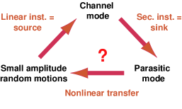
Figure 1: Cartoon of the process that may be at the origin of the saturation of the transport in shearing box simulations of MRI with a net vertical field (see text).

According to this picture, the channel modes linearly grow from random noise; at some amplitude, their growth is halted by a secondary instability (parasitic mode) which destroys the channel mode. Presumably, the parasitic modes themselves decay into small scale turbulence, which may then produce the seed for the random fluctuations out of which the channel mode grows in the first place. In this scenario, the channel mode(s) would be responsible for most of the transport, in particular near maxima of the transport fluctuations.

One of the objectives of this paper is to examine the relevance of this picture of MRI turbulence. Even if such a scenario is not generic (it depends directly on the presence of a mean vertical field), if confirmed, it might provide an interesting lead to analyze different situations. Another related objective it to assess the relevance of this scenario to the question of the Prandtl number dependence of MRI-driven transport. To this effect, we gather here the relevant pieces of information on the physics of channel modes that is required in order to analyze the simulations presented in the next section.

3.1 Dispersion relation

The physics of viscous and resistive channel modes has been examined in Lesur & Longaretti (2007) and their properties have been characterized in detail in Pessah & Chan (2008) (Sano & Miyama 1999 have also explored the role of resistivity on MRI in the absence of viscosity). Since non axisymmetric MRI modes are transiently growing structures in non ideal MHD (Balbus & Hawley, 1992), the axisymmetric modes give a good grasp of the linear stability properties of the shearing box.

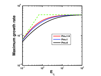
Figure 2: Maximal growth rate $\sigma_{M}/S$ as a function of the resistive dissipation, for the various values of the Prandtl number used in the simulations. Also shown are asymptotic analytic approximations (see text).

We recall here the dispersion relation of theses modes and a number of other features that will be of use in the next section.

Looking for solutions of the linearized equations of motions in the form $\bm{v}=\bm{v_{l}}\exp(\sigma t-ik_{y}y-ikz)$ and $\bm{b}=\bm{b_{l}}\exp(\sigma t-ikz)$ leads to the following fourth order dispersion relation:

$$\sigma^{4} +2k^{2}\sigma^{3}(\eta+\nu)+\sigma^{2}\Big{(}a+k^{4}(\eta^{2}+\nu^{2}+4\eta\nu)+b\Big{)}$$ (17)

$$+\sigma\Big{(}2k^{6}(\eta\nu^{2}+\nu\eta^{2})+ak^{2}(\nu+\eta)+2b\eta k^{2}\Big{)}$$

$$+\nu^{2}\eta^{2}k^{8}+a\nu\eta k^{4}+b\eta^{2}k^{4}-c=0,$$

with

$$a = 2k_{z}^{2}V_{A}^{2},$$ (18)

$$b = \kappa^{2}\gamma^{2},$$ (19)

$$c = k_{z}^{2}V_{A}^{2}(2\Omega S\gamma^{2}-k_{z}^{2}V_{A}^{2}),$$ (20)

and where $\kappa=[2\Omega(2\Omega-S)]^{1/2}$ is the epicyclic frequency, $V_{A}=B_{0}$ is the Alfvén speed based on the imposed mean vertical field, and $\gamma^{2}=k_{z}^{2}/(k_{y}^{2}+k_{z}^{2})$. Channel modes have $k_{y}=0$ so that $\gamma=1$.

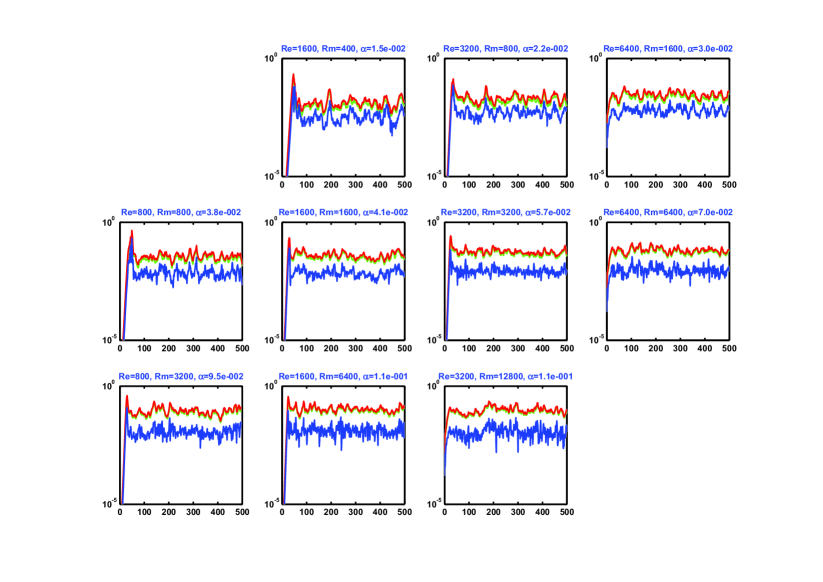
Figure 3: The dimensionless turbulent transport $\alpha$ as a function of time (in units of $S^{-1}$) for a vertical magnetic field strength $\beta=1000$ and various levels of viscous and resistive dissipation $Re$ and $Rm$. Insets on a given line correspond to constant magnetic Prandtl number, $Pm=1/4$, $1$ and $4$ from top to bottom. The Reynolds number $Re$ is constant on rows ($800$, $1600$, $3200$, and $6400$ respectively. The transport averages are computed over the last $400$ shear times of the simulations. The blue line represents the Reynolds stress, the green line the Maxwell stress, and the red line the total stress (these last two are almost indistinguishable).

This equation is used later on to compute the channel mode growth rates in the conditions of our numerical simulations. It is most conveniently solved in dimensionless form, with $S$ as unit of time and $V_{A}/S$ as unit of length. We introduce $\sigma^{*}=\sigma/S$, $\kappa^{*}=\kappa/S$, $k^{*}=V_{A}k/S$; defining the viscous ($E_{\nu}$) and resistive ($E_{\eta}$) Elsasser-like numbers by

$$E_{\nu} = \frac{V_{A}^{2}}{S\nu}=\frac{Re}{\beta}=\frac{\Lambda_{\nu}}{q},$$ (21)

$$E_{\eta} = \frac{V_{A}^{2}}{S\eta}=\frac{Rm}{\beta}=\frac{\Lambda_{\eta}}{q},$$ (22)

one has $\nu^{*}=1/E_{\nu}$ and $\eta^{*}=1/E_{\eta}$. Note that with a power-law velocity profile in a disk ($\Omega\propto r^{-q}$), $\Omega^{*}=1/q$ and $\kappa^{*}=[2(2-q)]^{1/2}/q$. Our definitions of the Elsasser numbers (and other dimensionless quantities) differ from the usual ones ($\Lambda_{\nu}$ and $\Lambda_{\eta}$, see e.g. Pessah & Chan 2008 and Pessah & Goodman 2009) by a factor $S/\Omega$. This choice has several motivations: $S$ rather than $\Omega$ is the relevant time-scale of linear growth rates; this definition is more consistent with our previous choice of units; and it makes the connection between the Elsasser and Reynolds numbers simpler.

3.2 Stability limits

In the dissipation-free limit, the dispersion relation can be solved exactly. The magnetic tension stabilizes the instability for $k^{*}>k_{c}^{*}\equiv(2\Omega^{*})^{1/2}=(2/q)^{1/2}$. In a box of finite vertical extent $L_{z}$, the vertical modes wavelengths are multiple of $k_{min}=2\pi/L_{z}$. Axisymmetric MRI modes are therefore stabilized when $k_{c}<k_{min}$, which translates into $\beta\geq\beta_{c}\equiv 2\pi^{2}S/\Omega\simeq 30$. The maximum growth rate in the dissipation-free regime, $\sigma_{M}=S/2$, is achieved for a wavenumber $k_{M}\simeq k_{c}/2$.

Resistivity and viscosity modify the marginal stability limit in the ($Re$, $Rm$, $\beta$) space. Numerical investigation indicates that only one of the four roots is unstable for $q<2$, so that the marginal stability limits obtains when the $\sigma$-independent term of the dispersion relation is equal to zero. Also, as shown by Lesur & Longaretti (2007), for $\beta\geq 100$ and $Re\gtrsim 400$ (two conditions that are satisfied in the present investigation), the marginal stability limit is nearly independent of the Reynolds number. This leads to the following expression of the marginal stability limit

$$Rm=\frac{\kappa\beta}{S}\left(\frac{\beta_{c}}{\beta-\beta_{c}}\right)^{1/2}=\frac{2\pi}{\sqrt{3}}\frac{\beta}{(\beta-\beta_{c})^{1/2}}\sim 3\beta^{1/2},$$ (23)

where the second equality applies for keplerian flows. The last approximation holds only when $\beta$ is large enough, and was given in Lesur & Longaretti (2007); the first expression is new and sensibly more precise.

The maximum growth rate achieved by the instability is modified when viscosity and resistivity become important, i.e. when either $E_{\nu}$ or $E_{\eta}$ $\lesssim 1$. Pessah & Chan (2008) give an asymptotic form of the growth rate in the dissipation regime for small or of order unity $Pm$ (see their Fig. 5 and their Eq. 91); it reads $\sigma_{M}=2\sigma_{0}E_{\eta}/3$ where $\sigma_{0}=S/2$ is the dissipation-free growth rate. The range of $E_{\eta}$ and $Pm$ examined in this work spans the transition from a dissipative to a non dissipative regime for the linear instability. The corresponding variation of maximum growth rate with both $E_{\eta}$ and $E_{\nu}$ (through the Prandtl number) is shown on Fig. 2, along with the asymptotic expressions just recalled.

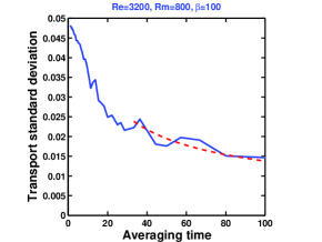
Figure 4: Transport standard deviation as a function of the time interval $\tau$ used to bin the transport data, for a given run (in this case, $Re=3200$, $Rm=800$, and $\beta=100$). This information is used to quantify the error in the transport from the fit $\propto\tau^{-1/2}$ that is expected to hold for large enough binning time $\tau$ (see text for details).

4 Numerical results

In order to explore a significant range of parameters, most of our runs are performed at a standard resolution ($N_{r}$, $N_{\phi}$, $N_{z}$) = (256, 128, 64) in real space. All simulations have an aspect ratio $R:\phi:z=4:4:1$; as argued earlier, this aspect ratio allows us to capture the fastest growing channel and parasitic modes. Three simulations have been performed at a resolution twice as large (512, 256, 128) in order to reach a higher Reynolds number ($Re=20000)$, and lower Prandtl numbers (down to $Pm=1/16$). Note that spectral codes are intrinsically more resolved than finite difference codes with the same number of points; as a consequence, one needs to adopt resolutions larger by a factor $\simeq 2$ in all directions in a finite difference code such as ZEUS, Athena or RAMSES to obtain the same results, a point to bear in mind when comparing our conclusions with those published in the literature with finite difference codes (see e.g. Fromang et al., 2007, for an explicit comparison).

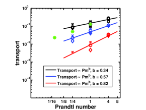
Figure 5: The dimensionless turbulent radial momentum transport $\alpha$ as a function of the Prandtl number $Pm$ and the field strength $\beta$ for various Reynolds numbers. black: $\beta=10^{2}$; blue: $\beta=10^{3}$; red: $\beta=10^{4}$; $\Box$: $Re=400$; +: $Re=800$; $\diamondsuit$: $Re=1600$; $\circ$: $Re=3200$; $\times$: $Re=6400$; the green starred data points correspond to the three more resolved runs at $Re=20000$ and $\beta=10^{3}$. Power law fits are also shown for each value of $\beta$.

The simulations performed in this work are in the large Reynolds number limit ($400<Re<20000$). The relevant marginal stability limit depends only on $Rm$ and is precisely given by Eq. (23). When the magnetic Reynolds number is too close to this limit, nonaxisymmetric perturbations damp out, and the flow becomes nearly identical to an axisymmetric one. We have checked that none of the simulations discussed below is affected by this issue.

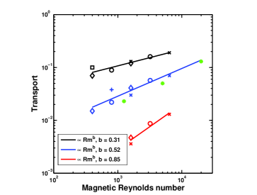
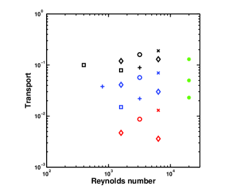
Figure 6: The dimensionless transport $\alpha$ as a function of the magnetic Reynolds number $Rm$ (left) and Reynolds number $Re$ (right). Black: $\beta=10^{2}$; blue: $\beta=10^{3}$; red: $\beta=10^{4}$; $\Box$: $R=400$; +: $R=800$; $\diamondsuit$: $R=1600$; $\circ$: $R=3200$; $\times$: $R=6400$; $R$ refers to $Re$ on the left panel, and to $Rm$ on the right one. The green stars correspond to the three more resolved runs at $Re=20000$ (see text).

With our adopted standard resolution, we can confidently resolve the dissipative scales up to Reynolds numbers $\simeq 10^{4}$. Consequently, we have explored Reynolds numbers in the range $400$ – $6400$ and magnetic Reynolds numbers in the range $400$ – $12800$. The magnetic Prandtl number of the simulations is either $1/4$, $1$ or $4$. A smaller value ($Pm=1/16$) has also been reached with one of our higher resolution runs with $Re=20000$.

We have performed simulations for three different vertical field strengths: $\beta=10^{2}$, $10^{3}$, and $10^{4}$. This range is constrained by two considerations. On the low end (large field), one must stay away from the marginal stability limit due to the magnetic tension. Indeed, when the incompressible MRI works too close to this stability threshold, the flow is strongly biased by the presence of channel modes (an effect that incompressible simulations are more prone to capture, as exemplified in Lesur & Longaretti 2007). On the large end (weak field), one is limited by the fact that at some point, the flow is going to be dominated by the zero flux transport process, whose dependence on the viscous and resistive dissipation might be sensibly different. If one simply assumes that one shifts from one regime to the other when the efficiency of the transport processes are equal, one finds that the transition between the mean field and zero net field regimes should be in the range $\beta\sim 10^{5}$ – $10^{4}$; this limit applies to $Pm\gtrsim 2$ (as the zero net flux transport vanishes for lower Prandtl number values), and should be somewhat dependent on $Pm$. As discussed later on, for our weakest field ($\beta=10^{4}$) and smallest Prandtl ($Pm=4$), the flow also tends to become bidimensional for low enough Reynolds number.

4.1 Transport time histories and standard deviation

Figure 3 displays the behavior of the turbulent transport for the runs we have performed at $\beta=1000$. The simulations are typically run for $500$ shear times, and the transport average is based on the last $400$. In our horizontally extended simulation boxes, the transport fluctuations are substantially reduced with respect to narrower boxes. Typically, fluctuations of a factor of $\sim 2$ are observed, whereas in $r:z=1:1$ boxes, fluctuations of an order of magnitude or more are common. This reduction provides more precise averages for the transport, even though the averaging time is somewhat smaller than what is used for boxes with a $R:Z=1:1$ aspect ratio. This aspect ratio dependence is related to the prominence of channel modes in the large transport bursts observed in the narrow boxes (Bodo et al., 2008), a feature related to the fact that width of the narrow box is comparable to the correlation length of turbulent fluctuations in the horizontal direction (Guan et al., 2009).

The transport time history can be used to quantify the error in the determination of $\alpha$ in the following way. From the raw time history, one can define a series of binned time histories, with a binning time $\tau$ ranging from $1$ to $100$ shear times. From these binned time histories, one can define a transport standard deviation in the usual way, i.e., $\sigma_{\alpha}=[\sum(\alpha_{i}-\overline{\alpha})^{2}/N]^{1/2}$ where $N$ is the number of bins, $\alpha_{i}$ itself being the average value of the transport in bin $i$. The resulting dependence $\sigma_{\alpha}(\tau)$ is shown on Fig. 4 for one of our runs. Two regimes can be distinguished. For $\tau\lesssim 10$ – $20\ S^{-1}$, the deviation decreases sharply with $\tau$; this is seen directly on Fig. 3, where the transport typical variation time scale is precisely in this range. For large values of $\tau$, the transport is less and less correlated with itself. Consequently, one expects that it should behave more or less as a random walk, so that the standard deviation should scale like $\tau^{-1/2}$. A fit of this type is performed on Fig. 4, and appears to represent reasonably well the trend, in spite of the crudeness of the approximation.

From this approximation we find that the relative error in the computation of the transport over $400$ shear times is in the range $3$ – $10\%$. There is no clear tendency for the larger values of the relative error to correspond to higher transport, and no clear trend with either the magnetic Prandtl or magnetic Reynolds number. On average, $\sigma_{\alpha}/\alpha\sim 5\%$.

4.2 Physical dissipation and transport

The dependence of the transport on the dissipation for various field strengths is presented on Fig. 5 for all our standard resolution runs. This figure significantly extends the results reported in (Lesur & Longaretti, 2007). Several trends can be observed:

• For a given field strength, the dependence on the magnetic Prandtl number $Pm$ seems to follow an approximate power law. For comparison with our previous work, power-law fits are computed. The exponents are $\simeq 0.3$, $0.7$ and $0.8$ for the three values of $\beta$, in increasing order.

• The three more resolved runs confirm this trend: the transport is substantially larger than other runs at the same field strength ($\beta=10^{3}$), but the $Pm$ dependence is consistent with the other runs at the same $\beta$; this $Pm$ dependence does not seem to saturate even though a lower Prandtl number has been achieved (1/16).

• At a given Prandtl number, the transport is decreasing with decreasing field strength (increasing $\beta$). This trend is expected from the scaling $\alpha\propto\beta^{-1/2}$ that was first pointed out in the initial work of Hawley et al. (1995). However, the variation of the index of the Prandtl number dependence with field strength just discussed induces deviations from this scaling.

• There is a weaker, but systematic and significant increase of the transport with increasing Reynolds number at any given field strength and Prandtl number. This effect is real: for most of our runs, this increase is larger than the standard deviation in the transport, as quantified in the previous subsection. It is also larger for the smaller Prandtl number values. This indicates that the Prandtl number does not capture all the physics of the correlation between transport and physical dissipation; this point is further discussed below.

Our previous investigation was limited to $\beta=100$. In the present work, the Prandtl number dependence of the transport for this field strength is consistent with our earlier findings. However, the transport observed here is reduced by a factor $\sim 2$; this is a direct consequence of the reduced role played by the channel mode in our horizontally extended simulation boxes.

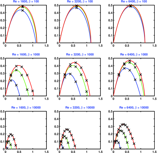
Figure 7: Composite figures showing the dimensionless growth rate $\sigma/S$ of the channel mode for most of the various runs performed, as a function of the dimensionless wavenumber $V_{A}k_{z}/S$. Each subplot is labelled by its Reynolds number and field strength ($\beta$). The various curves in each subplot correspond to $Pm=1/4$, $1$, $4$, respectively (the growth rate increases with increasing Prandtl number). The crosses indicate the modes that are represented in our simulation boxes, as a result of the boundary conditions (see text for a discussion).

For the lowest Prandtl number ($1/4$) and lowest field strength ($\beta=10^{4}$), only one point is reported in the graph. Our other runs for this parameter have lower Reynolds numbers, and are too close to the linear stability threshold of Eq. (23) to sustain full 3D turbulent motions. These runs show 2D or quasi-2D behavior, with very different transport efficiency and behavior. The data point we have retained might still be weakly affected by such effects.

As pointed out above, Fig. 5 indicates that the spread with Reynolds number at a given Prandtl number increases with decreasing Prandtl number. In fact, two different regimes can be noted, one for $Pm\leq 1$ and one for $Pm=4$.

At $Pm=4$, the transport seems to be only weakly dependent on $Re$ (or $Rm$), at least for large enough Reynolds number: the transport increases by $10\%$ to $50\%$ (depending on $\beta$) while the Reynolds number is multiplied by a factor of 4. This trend can also be found in the work of Simon & Hawley (2009), where the MRI turbulent transport in presence of a toroidal field is investigated with more emphasis on the $Pm>1$ regime. Their Figs. 6 and 7 show that, for $Pm=2$ and $4$ at least (the only ones with enough data in the $Pm>1$ regime), the transport increases steadily with the Reynolds number for $Re\lesssim 1000$ and much more weakly for $Re\gtrsim 1000$.

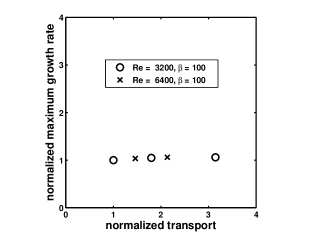
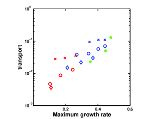
Figure 8: The relation between dimensionless turbulent radial momentum transport $\alpha$ and the dimensionless growth rate $\sigma/S$. There is no correlation at the largest $\beta$ and $Re$ (left) while there is one for weaker field strengths (right). In the left panel, the transport and growth rate of the $Re=3200$, $Pm=1/4$ run have been used to normalize the data. Black: $\beta=10^{2}$; blue: $\beta=10^{3}$; red: $\beta=10^{4}$; $\diamondsuit$: $Pm=1/4$; $\circ$: $Pm=1$; $\times$: $Pm=4$. The three resolved runs are also shown (green stars).

On the contrary, the spread in Reynolds number for $Pm\leq 1$ is substantial, and systematic. Such a spread was not detected in our earlier investigation, due to the larger fluctuations in transport related to the box aspect ratio, as discussed earlier. In fact, this dispersion seems to be an effect of the magnetic Reynolds number. To illustrate this point, the transport is represented on Fig. 6 as a function of $Rm$ (left panel) and $Re$ (right panel), for $Pm\leq 1$; the colors describe different field strengths ($\beta=10^{2}$ to $10^{4}$ from top to bottom). The statistics in the number of points at any given $Re$ or $Rm$ is rather low; however, it appears quite clearly that the dispersion of the points at any given Reynolds number is substantially larger in $Re$ (with varying $Rm$) than in $Rm$ (with varying $Re$). The largest Reynolds number data strongly support this conclusion. Furthermore, the fits of the transport as a function of $Rm$ indicate the $Rm$ dependence of the transport for $Pm\leq 1$ is very similar to its $Pm$ dependence as shown on Fig. 5. This strongly suggests that the $Pm$ dependence observed on this figure is in fact mostly a $Rm$ dependence for $Pm\leq 1$. Including the $Pm=4$ data destroys this correlation, which strengthens the idea that there are two regimes, depending on the Prandtl number (a feature that may be related to the existence of a transition around $Pm=2$ in zero net flux shearing box simulations). The relevant results of Simon & Hawley (2009); although less detailed, are consistent with these findings (see their Fig. 7).

5 Role of channel and parasitic modes

5.1 Linear physics and turbulent transport

Lesur & Longaretti (2007) concluded that there was no direct connection between the Prandtl dependence of MRI-driven turbulent transport and the linear growth rate of channel modes. However, the transport was substantially less precisely determined than in the present investigation, and the issue is worth reinvestigating.

To this effect, one needs to compute the linear instability growth rates for the various runs we have performed. We focus on the growth rate of the channel mode; for one thing, it is a guideline for the stability behavior of all unstable modes, and for another, there is a particular interest in the behavior of this specific mode. The resulting growth rates are numerically computed from the dispersion relation recalled in section 3.1 and represented in Fig. 7. The important features to note from this figure are the following:

• The largest growth rate in the continuum limit is always represented or very nearly represented in the simulation, in spite of the discreteness imposed by the vertical boundary condition (the corresponding modes are shown by crosses on the figure). This ensures that the fastest growing channel mode is always present in our simulations.

• For the largest field strength ($\beta=100$), the growth rates of all our simulations is very close to the ideal MHD limit ($\sigma=S/2$). This is especially true of the two largest Reynolds numbers ($Re=3200$ and $Re=6400$). Note in particular for these runs that the growth rate changes by at most $10\%$ while the transport varies by a factor of more than $3$ (see left panel of Fig.. 8). As a consequence the existence of the Prandtl and magnetic Reynolds number dependences of the transport is not related to the variation of the growth rate with physical dissipation.

• For $\beta=1000$, and for the two largest Prandtl numbers ($Pm=1$ and $Pm=4$) and largest Reynolds numbers ($Re=3200$ and $Re=6400$), the growth rate is again almost independent of the dissipation. As there is only one captured channel mode for the $\beta=100$ vs four or five for $\beta=1000$, the $Pm,Rm$ dependence is not related to the number of captured channel modes in the simulation.

There is a sharp behavior difference of the transport with respect to the linear MRI growth rate between the nearly ideal simulations performed at $\beta=100$ and the lower $\beta$ values, as is apparent when comparing the left and right panels of Fig. 8. In fact, the whole spectrum of possible behaviors is covered here, from substantial variation of the transport with very weakly varying growth rates (left panel), or conversely substantial variation of the growth rate while the transport is only weakly or mildly changing ($Pm=4$ data on the right panel) and intermediate situations where the two are more strongly correlated (the other data points on the right panel). Therefore, although this situation is more contrasted than indicated in Lesur & Longaretti (2007), the conclusion stands: there is no clear and direct relation between the effects of dissipation on linear physics and the nonlinear turbulent saturation mechanism.

5.2 Quasi-linear physics and turbulent transport:

As indicated in the introduction and in section 3, it is often assumed that the channel mode is responsible for most of the MRI-driven turbulent transport in the presence of a net vertical magnetic field. In particular Pessah & Goodman (2009) argue that the saturation of the channel mode by its parasites may help us to understand the transport. In this section, we make use of our numerical results to investigate these issues.

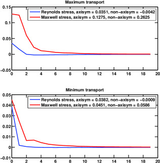
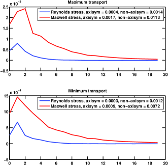
Figure 9: One-dimensional spectrum of the transport, in the azimuthal direction, as a function of the wavenumber $n_{\phi}$ such that $k_{\phi}=2\pi n_{\phi}/L_{\phi}$. $\beta=10^{2}$ for the two left figures, and $\beta=10^{4}$ for the two right ones. The upper plots correspond in each case to a typical transport maximum in the time history, while the lower ones describe a typical minimum. Both the Reynolds and Maxwell stress are shown. The transport due to non-axisymmetric modes always dominates the transport due to the axisymmetric ones (channel modes). See text.

We first disprove the first statement: the channel mode does not clearly dominate transport, especially at the maxima of the transport, as should in the scheme depicted on Fig. 1. This is shown explicitly in Fig. 9. A one-dimensional Fourier transform of both the Maxwell and Reynolds stress along the azimuthal direction is shown in this figure. These transforms are performed at a typical minimum and maximum of transport in the transport history of two of our runs, namely the runs with $Re=Rm=6400$ at $\beta=100$ and $\beta=10^{4}$, respectively. The transform is shown in terms of the wavenumber $n=k_{\phi}L_{\phi}/2\pi$; $n=0$ corresponds to the transport due to the axisymmetric modes (channel modes) present in the simulations, for the various captured $k_{z}$. The other wavenumbers ($n\neq 0$) correspond to non-axisymmetric modes. Channel modes dominate over other individual wavenumbers for $\beta=100$. However, the cumulated contribution of non-axisymmetric modes is dominant by a factor $\lesssim 2$ at the maximum of transport for this $\beta$, and does not exceed the non-axisymmetric contribution by more than $\sim 30\%$ at minimum transport. For $\beta=10^{4}$, the cumulated non-axisymmetric are always dominant by a factor $\sim 6$. For $\beta=10^{3}$ (not shown), the situation is somewhat intermediate between the two extreme values presented in the figure, but the non-axisymmetric contribution is again always dominant by a factor several.

In summary, except for minimum transport for the largest field strength where axisymmetric and non-axisymmetric contributions to the transport are comparable, the non-axisymmetric contribution is always larger by a factor $\sim 5$. As a result, it seems necessary at least to include non-axisymmetric modes in the process sketched on Fig. 1.

Furthermore, the analysis of Pessah & Goodman (2009) is inconsistent with our results, both from a qualitative and quantitative point of view. Our simulations always capture the fastest growing channel mode, or very nearly so (see Fig. 7). Due to the choice of aspect ratio, the fastest growing parasitic modes are always captured as well. Finally, for $\beta=100$ and $Re=3200$ and $6400$ (even $1600$ for the two larger $Pm$ values), the variation of the transport with $Pm$ is quite substantial, whereas Pessah & Goodman (2009) conclude that in these conditions, the transport is independent of dissipation (see the left plot in Fig. 2 of their paper; the three Reynolds numbers values mentioned correspond to the three largest Elsasser numbers of their graph).

6 Discussion and conclusion

Perhaps the most significant new result of this work, disclosed on Figs. 5 and 6, is the existence of a double regime separated by a critical magnetic Prandtl number $Pm_{c}\sim 1$. For $Pm<Pm_{c}$, at a given field strength, the transport correlates mostly with $Rm$; for $Pm>Pm_{c}$, the transport seems to depend mostly on $Pm$ and only weakly on either $Re$ or $Rm$ (once $Re\gtrsim 10^{3}$), although a larger number of $Pm$ values need to be probed on this issue. It is tempting to assume $Pm_{c}\simeq 2$, as this is the critical value for the zero mean field problem, but this identification requires further work to be substantiated. The identification of this double dissipation regime was made possible by the increased accuracy, with respect to our previous work, in the determination of the transport averages. In the small Prandtl regime, in contrast to the large one, our most resolved simulations show no sign of convergence with respect to dissipation, although values of $Rm$ up to 20000 have been reached.

The role of linear physics and parasitic modes on transport properties has also been investigated, and the major results on these questions can be summarized as follows:

• The existence of the dependence of turbulent transport on dissipation is not related to the role of dissipation on linear modes growth rates.

• The existence of the correlation of transport with dissipation is not related to the number of channel modes captured in the simulations.

• Saturation of the channel modes growth by parasitic modes is not the responsible for correlation of transport with dissipation. This is hardly surprising as both the channel and parasitic modes are large scale modes, that are expected to be little affected by dissipation, whereas the trends of the transport with dissipation are substantial.

• Furthermore, the transport is usually not dominated by axisymmetric modes; these modes contribute at most at the same level as non-axisymmetric modes for the strongest fields investigated, and have negligible contributions for the weakest fields.

Note that all these results were obtained while the fastest growing channel and parasitic modes were always captured, so that they do not depend on limitations on this front.

It is worth pointing out that our results do not totally disqualify a saturation of the unstable linear modes by the parasitic modes; only the relevance of this process to the relation between transport and physical dissipation has been disproved.

The role of the Prandtl number disclosed in this investigation makes more physical sense than a direct dependence of the transport on $Pm$. Indeed, it is very likely that the critical value $Pm_{c}$ relates to the switching of the magnetic and kinetic dissipations scales $k_{\eta}$ and $k_{\nu}$ in Fourier space: for $Pm<Pm_{c}$ (resp. $Pm>Pm_{c}$), $k_{\eta}<k_{\nu}$ (resp. $k_{\eta}>k_{\nu}$). For $Pm\ll 1$, $k_{\eta}\ll k_{\nu}$, the flow at scales $k>$ or $\gg k_{\eta}$ in Fourier space is therefore purely hydrodynamic. As information flows from small $k$ to large $k$ in this scale range, the flow should be independent of $Re$, so that in this regime $\alpha=\alpha(\beta,Rm)$ is expected. The transport may even become independent of $Rm$ at large enough $Rm$ in the absence of backreaction of the small scales on the large ones, and if energy exchanges are not strongly nonlocal in Fourier space. We merely note here that in the context of homogeneous, isotropic, incompressible MHD turbulence, all energy transfers are direct (from small $k$ to large $k$); exchanges between magnetic and kinetic energy are nonlocal in Fourier space (Alexakis et al., 2007), although this nonlocality seems to be of finite (albeit large) extent (Aluie & Eyink, 2009). The situation is more complex in the large Prandtl regime, as non-local transfers and small scale dynamo action might take place at scales smaller than the viscous dissipation scale, and further investigations are required to characterize the properties of the small dissipation limit, in particular concerning the locality of transfers.

The behavior of MRI-driven turbulence with respect to these various issues will be reported elsewhere, through the analysis of energy transfers in Fourier space. More generally, investigating the possible independence of transport with respect to dissipation in the $Pm\ll Pm_{c}$ or $Pm\gg Pm_{c}$ limits requires to achieve a double scale separation: one must first separate in Fourier space the smallest injection scales (the scales which contribute to the Reynolds and Maxwell stresses) from the largest dissipation scales, and then the two dissipation scales themselves. This is extremely demanding in terms of resolution. Our simulations in the small Prandtl regime are consistent with a separation of dissipation scales nearly achieved. As a first step at small Prandtl (the most critical regime for YSO disks), one can achieve one or the other of the two scales separation. Such investigations are underway and will be reported elsewhere.

These questions are critical for astrophysical disk dynamics, where the Reynolds numbers are always very large ($Re\gtrsim 10^{10}$, while the Prandtl number spans very small ($\lesssim 10^{-5}$, YSO disks) to very large values ($\gtrsim 10^{5}$, AGN disks). Addressing these issues requires to overcome a number of limitations in the simulations. Besides the questions of scale separation and nonlocality of transfers in Fourier space just mentioned, the role of compressibility and vertical stratification on these results must be quantified. These questions can certainly be investigated in shearing boxes, but global simulations are probably still largely out of reach, due to the resolution demand. Also (and probably as much importantly), different dissipation regimes must be analyzed in the context of YSOs, namely the ambipolar and Hall regime, which are known to have substantial effect on the linear development of the MRI, while being relevant for large fractions of YSO disks.