Analysis and optimization of a free-electron laser
with an irregular waveguide

Abstract

Using a time-dependent approach the analysis and optimization of a planar FEL-amplifier with an axial magnetic field and an irregular waveguide is performed. By applying methods of nonlinear dynamics three-dimensional equations of motion and the excitation equation are partly integrated in an analytical way. As a result, a self-consistent reduced model of the FEL is built in special phase space. The reduced model is the generalization of the Colson-Bonifacio model and takes into account the intricate dynamics of electrons in the pump magnetic field and the intramode scattering in the irregular waveguide. The reduced model and concepts of evolutionary computation are used to find optimal waveguide profiles. The numerical simulation of the original non-simplified model is performed to check the effectiveness of found optimal profiles. The FEL parameters are chosen to be close to the parameters of the experiment (S. Cheng et al. IEEE Trans. Plasma Sci. 1996, vol. 24, p. 750), in which a sheet electron beam with the moderate thickness interacts with the TE₀₁ mode of a rectangular waveguide. The results strongly indicate that one can improve the efficiency by a factor of five or six if the FEL operates in the magnetoresonance regime and if the irregular waveguide with the optimized profile is used.

I Introduction

The recent progress in the theory and experiment of free-electron lasers (FELs) and gyrotrons Ginzburg et al. (2000); Sirigiri et al. (2001) with Bragg cavities is strongly indicative that the application of novel electrodynamical structures provides the opportunity to realize unique properties of FELs to a large measure. For example, Bragg cavities, which are periodic arrays of varying dielectric or metallic structures, stimulate interest in traditional microwave applications because they can be built oversized (quasioptical) and, therefore, employed at higher frequencies and higher power. At the same time the investigation of traveling wave tubes (TWT) Kravchenko et al. (2007) shows that the TWT efficiency based on a regular (along the interaction region) electrodynamical structure is far from its possible maximal value. In fact, the difference between the cold phase velocity and the average velocity of the beam is the control parameter of the beam-wave interaction. By changing this parameter along the interaction region one can control the beam bunching and the energy transfer between bunches and microwaves. The local variation of the cold phase velocity along the region depends on the local variation in the waveguide profile. Then, in an effort to control the beam-wave interaction and improve the efficiency one should use irregular electrodynamic structures. Specifically, the combination of Bragg reflectors Bratman et al. (1983) and the section of an irregular waveguide seems to be a promising electrodynamic structure for a high-efficiency powerful FEL. The analysis of a planar FEL-amplifier with an axial magnetic field and an irregular waveguide is the topic of the present paper. I focus my attention on this FEL configuration because it is well known that through the use of the axial magnetic field one can substantially improve the efficiency, as the cyclotron frequency tends to the undulator frequency Sprangle and Granatstein (1978).

It is worth noting that in vacuum electronic sources of coherent radiation the electron beams are far from the statistical equilibrium and during their interaction with radiation they remain sufficiently nonequilibrium because of the large free length Vainshtein and Solntsev (1973); Davidson (2001). Thus, the efficiency of the transfer of the electrons’ kinetic energy into radiation, basically, may be close to 100% (the klystron or traveling wave tube are the examples of high-efficiency devices) and the challenge is to optimize the beam-wave interaction by controlling the most important parameters. There are several ways to improve the FEL efficiency: optimization of electron beam characteristics (for example, development of beams with the optimal distribution of the axial velocity across a beam when the effect of beam finite thickness is relevant), tapering of the undulator or the axial magnetic field, profiling of waveguide/resonantor walls. In particular, the effectiveness and reliability of the undulator tapering were demonstrated theoretically Kroll et al. (1981); Freund and Gold (1984) and confirmed experimentally to a great advantage. In the experiment Orzechowski et al. (1986) the saturated power of 180 MW (6% efficiency) has been increased to 1.0 GW (34% efficiency) by optimizing the wiggler profile in such a way that the beam-wave resonance condition remains fulfilled for many electrons, as the electrons lose their energy. The numerical simulation mentioned in Orzechowski et al. (1986) indicates that one can trap about 75% of the electron beam and reduce its energy by about 45%. A high effectiveness of the undulator tapering was also demonstrated for a FEL with an axial guide magnetic field Freund and Ganguly (1986a) (the maximum efficiency was increased by almost 700% as compared to the untapered configuration). At the same time there exist cases where the convenient undulator profiling cannot be used or ensure desired enhancement. In particular, if the waveguide backward mode is used as an electromagnetic undulator, then, clearly, one has to change electrodynamic structure characteristics to control electromagnetic undulator parameters. The optimization of the electromagnetic structure also seems to be more efficient than the undulator profiling if the effect of the electron beam finite thickness is relevant. Indeed, given the FEL amplifier operates with Group II orbit parameters, a negative masslike effect occurs Freund and Antonsen (1995) in which the electrons are axially accelerated, as they lose energy to the wave. Hence, the electrons must be decelerated to maintain the beam-wave resonance. This is accomplished by an upward taper in the undulator field Freund and Ganguly (1986a). At the same time, the electrons with different initial transverse positions are exposed to the action of different magnitudes of the pump magnetic field. As a result, the average velocity of the electron depends on its initial transverse position, and different beam layers have different detunings with the wave because the average velocity of the electron governs the initial detuning. If the undulator field is tapered ‘up’, then the detuning of external layers of a thick beam increases and the contribution of these layer to the total efficiency shows a certain decrease. In the present paper I demonstrate that one can effectively suppress layering and the saturation efficiency effect by using the optimized profiled waveguide. I believe this technique to be useful for the development of powerful thick-beam FELs (for example the FEM experiments Sinitsky et al. (2009) on generation and transport of two intense beams have been performed of late: 0.8 MeV electron energy, current densities of up to 1.5 kA/cm², 0.4 $\times$ 7.0 cm² beam cross sections).

This paper is structured as follows: in Sec. II the problem statement for the planar FEL-amplifier with the axial magnetic field and the irregular waveguide is defined. The integrals of motion for a test electron in the pump magnetic field are constructed in Sec. III. With these integrals and the method of nonlinear resonance the FEL reduced model is derived in Sec. IV. In the following section the principle of the beam-wave control are considered and a practical example of the optimized FEL is given. The obtained results are discussed in Summary, and, finally, the wave interaction in the irregular waveguide is examined in Appendices A and B.

II The theoretical model

Let a sheet relativistic electron beam be injected into an irregular waveguide located in the external pump magnetic field that consists of the magnetic field of a linearly polarized (planar) undulator and a uniform axial magnetic field (see Fig. 1). The pump magnetic field is given by the vector-potential:

$${A}_{x}^{p}(\vec{r})=(B_{u}/k_{u})\cosh(k_{u}y)\cos(k_{u}z)+B_{\|}y.$$ (1)

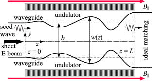
Figure 1: Sketch of the FEL in the $x=0$ cross section.

Here $B_{\|}$ is the uniform axial guide field, $B_{u}$ is the magnitude of the planar undulator field Booske et al. (1994), $k_{u}=2\pi/\lambda_{u}$ and $\lambda_{u}$ are the wave number and the period of the undulator, respectively. In numerical simulations we model the injection of the electron beam into the interaction region by allowing the undulator amplitude to increase adiabatically from zero to a constant level over $N_{u}$ undulator periods Freund et al. (1987). The unmodulated electron beam enters the interaction region, $z\in[0,L]$, with average longitudinal velocity $V_{\|}$. The irregular waveguide boundaries are set by expressions: $x=\pm a/2$ and $y=\pm w(z)/2$ ($a\gg w$), where $w(z)$ describes the varying distance between two wide walls of the waveguide, and $w^{\prime}(0)=w^{\prime}(L)=0$. Let the FEL-amplifier be seeded by the TE₀₁ mode, which is resonant (synchronous) with the electron beam, the mode frequency and the amplitude at the input into the interaction region ($z=0$) equaling $\omega$ and $V_{0}$, respectively. We consider that the interaction region is ideally matched to the regular output waveguide at the section $z=L$.

Since the narrow walls are profiled, $y=\pm w(z)/2$, one can apply the local Fourier-series expansion Makarov and Tarasov (2001) over $y$ to derive the coupled set of equations governing the evolution of TE_nm and TM_nm modes (subscripts $n$ and $m$ correspond to the field variation along the wide and narrow walls, respectively). Modes with odd TE_n,odd, TM_n,odd and even TE_n,even, TM_n,even variations are not coupled because of the waveguide symmetry with respect to $xz$-plane. We will hold that $\lambda>2w(z)/3$, and the TE_0m modes for $m>3$ are then evanescent and the scattering of the seed TE₀₁ mode to those modes will be neglected. We also ignore the electron beam mode generation. Under this assumptions the evolution of the signal TE₀₁ mode is governed by the $x$-component of vector-potential $A_{x}^{s}$:

$$A_{x}^{s}(\vec{r},t)=\mathrm{Re}\Bigl{\{}V(z,t)\sqrt{\frac{b}{w(z)}}\cos\Bigl{(}\frac{\pi y}{w(z)}\Bigr{)}\,e^{-i\omega t}\Bigr{\}}.$$ (2)

Here $V(z,t)$ is the slow-in-time amplitude satisfying the equation (see A)

$$\Bigl{\{}\frac{\partial^{2}}{\partial z^{2}}+k_{z}^{2}+\frac{2ik_{z}}{v_{gr}}\frac{\partial}{\partial t}\Bigl{\}}V(z,t)=-\frac{8\omega}{Sc}\sqrt{\frac{b}{w(z)}}\int_{-a/2}^{a/2}dx\times\\ \int_{-w(z)/2}^{w(z)/2}dy\int_{t-\pi/\omega}^{t+\pi/\omega}dt^{\prime}\,j_{x}(\vec{r},t^{\prime})\cos\Bigl{(}\frac{\pi y}{w(z)}\Bigr{)}e^{i\omega t^{\prime}},$$ (3)

where

$$k_{z}^{2}(z)=\frac{\omega^{2}}{c^{2}}-\Bigl{(}\frac{\pi}{w(z)}\Bigr{)}^{2}-\Bigl{(}\frac{w^{\prime}(z)}{2w(z)}\Bigr{)}^{2}\Bigl{[}1+\frac{\pi^{2}}{3}\Bigr{]}$$

is the wave number squared, $v_{gr}(z,\omega)=(dk_{z}/d\omega)^{-1}$ is the group velocity, $c$ is the speed of light and $S=a\times b$. The boundary conditions read

$$\begin{split}&\Bigl{(}\frac{\partial V}{\partial z}+ik_{z}V-\frac{1}{v_{gr}}\frac{\partial V}{\partial t}\Bigr{)}\Bigr{|}_{z=0}=2ik_{z}V_{0},\\ &\Bigl{(}\frac{\partial V}{\partial z}-ik_{z}V+\frac{1}{v_{gr}}\frac{\partial V}{\partial t}\Bigr{)}\Bigr{|}_{z=L}=0.\end{split}$$ (4)

The microscopic current density is given by the following sum over electron trajectories, Freund et al. (1987):

$$\vec{j}(\vec{r},t)=\frac{I_{0}}{S_{b}}\!\!\int\limits_{-X_{b}/2}^{X_{b}/2}\!\!dx_{0}\!\!\int\limits_{-Y_{b}/2}^{Y_{b}/2}\!\!dy_{0}\!\!\int\limits_{t-L/V_{\|}}^{t}\!\!dt_{e}\frac{\vec{p}(z;\vec{r\;}_{\perp 0},t_{e})}{p_{z}(z;\vec{r\;}_{\perp 0},t_{e})}\times\\ \delta[\vec{r}_{\perp}-\vec{r}_{\perp}(z;\vec{r\;}_{\perp 0},t_{e})]\delta[t-t(z;\vec{r\;}_{\perp 0},t_{e})],$$ (5)

where $I_{0}$ is the beam current at the input into the interaction region; $S_{b}=X_{b}Y_{b}$ is the cross sectional area of the beam; $\vec{p}(z;\vec{r}_{\perp 0},t_{e})$ and $\vec{r}_{\perp}(z;\vec{r}_{\perp 0},t_{e})$ are the mechanical momentum and the transverse coordinate, respectively; $t(z;\vec{r}_{\perp 0},t_{e})$ is the arrival time of an electron at the position $z$; $t_{e}$ and $\vec{r}_{\perp 0}=\vec{r}_{\perp 0}(x_{0},y_{0})$ are the entrance time and the transverse coordinates, which the electron has at the input of the interaction region. The sheet electron beam is lying from $x_{0}=-X_{b}/2$ to $x_{0}=X_{b}/2$ and from $y_{0}=-Y_{b}/2$ to $y_{0}=Y_{b}/2$ in the $x$ and $y$ directions, respectively. Since the relativistic electron-wave interaction is being studied, the nonradiated fields (space-charge fields) are supposed to be negligible. The relativistic effects result in that the force $f_{m}$ caused by the nonradiated magnetic field partially suppresses the defocusing action of the transversal part of the force $f_{e}^{(pot)}$ caused by the potential part of the nonradiated electric field, the axial component of $f_{e}^{(pot)}$ being partially compensated by the force $f_{e}^{(rot)}$ caused by the rotational part of the nonradiated electric field (see Goryashko et al. (2009) for details).

The motion of a typical electron within the electron beam can be described by the relativistic Hamiltonian

$$\mathcal{H}=\sqrt{m_{e}^{2}c^{4}+\bigl{(}c\vec{P}-e\vec{A}^{p}-e\vec{A}^{s}\bigr{)}^{2}}=m_{e}\gamma c^{2}.$$ (6)

Here $e$ and $m_{e}$ are the electron charge and rest mass, respectively; the canonical momentum $\vec{P}$ is related to the mechanical momentum $\vec{p}$ by $\vec{P}=\vec{p}+(e/c)(\vec{A}^{p}+\vec{A}^{s})$. The initial conditions for the mechanical momentum and coordinates read:

$$p_{x}|_{t=t_{e}}=p_{y}|_{t=t_{e}}=0,\quad p_{z}|_{t=t_{e}}=\mathcal{E}V_{\|}/c^{2},$$ (7)

$$x|_{t=t_{e}}=x_{0},\quad y|_{t=t_{e}}=y_{0},\quad z|_{t=t_{e}}=0,$$

where $\mathcal{E}$ is the initial energy of the electron entering the interaction region at the time $t_{e}$. The excitation equation (3) along with the expression for the current density (5) and the equations of motion generated by the Hamiltonian (6) describe the electron-wave interaction in the studied FEL in a self-consistent way. In the self-consistent models the main mathematical obstructions are due to the nonlinear character of the equations of motion, and in order to perform the analytical treatment of the FEL we first have to integrate the equations of motion generated by the Hamiltonian (6). For the purpose of subsequent analysis, it is convenient to rewrite the Eq. (6) as

$$\mathcal{H}(\vec{r},\vec{P},t)=\sqrt{\bar{\mathcal{H}}^{2}(\vec{r},\vec{P})+W(\vec{r},\vec{P},t)},$$ (8)

where $\bar{\mathcal{H}}$ describes the dynamics of a typical electron in the pump magnetic field

$$\bar{\mathcal{H}}=\Bigl{[}\bigl{\{}cP_{x}-e[(B_{u}/k_{u})\cosh(k_{u}y)\cos(k_{u}z)+B_{\|}y]\bigr{\}}^{2}+\\ (cP_{y})^{2}+(cP_{z})^{2}+m_{e}^{2}c^{4}\Bigr{]}^{1/2}=m_{e}\gamma_{0}c^{2},$$ (9)

and the ponderomotive perturbation reads

$$W=-2e(cP_{x}-eA_{x}^{p})A_{x}^{s}+(eA_{x}^{s})^{2}.$$ (10)

We start our analysis with the integration of the equation of motion generated by the unperturbed Hamiltonian (9). The above integration is the nontrivial problem because the nonlinear dynamical system (9) is not globally integrable Michel-Lours et al. (1993) and exhibits chaotic behavior if the absolute value of the difference between the normal undulator and normal cyclotron frequencies is less than the betatron frequency Goryashko et al. (2009). The dynamics of electrons in an ideal undulator and an axial magnetic field was studied in details in Ref. Goryashko et al. (2009) using Lindshtedt’s perturbation method in configuration space. This allowed one to build a linear microwave theory and analyze the electron-wave interaction in the magnetoresonance regime. However, to build the nonlinear theory we have to study the behaviour of a test electron in the pump magnetic field in a more specific way. In the next section we build the approximate solution for (9) by means of the superconvergence method in action-angle variable space and derives the explicit analytical expressions for the region location of chaotic dynamics in the parameter space.

III Dynamics of electrons in the pump magnetic field

III.1 Action-angle variables formulation

In order to apply the perturbation method to the nonlinear system with the Hamiltonian (9) the latter is divided into a nonperturbed (integrable) part that corresponds to the electron motion in the axial homogeneous magnetic field and a small perturbation caused by the undulator magnetic field. Based on the nonperturbed system (the undulator field is absent $B_{u}=0$) we can introduce the action-angle variables:

$$P_{y} =-\frac{\sqrt{2\omega_{c}\mathcal{E}I_{c}}}{c}\sin\vartheta_{c},\qquad P_{z} =k_{u}I_{u},$$ (11)

$$y =c\sqrt{\frac{2I_{c}}{\omega_{c}\mathcal{E}}}\cos\vartheta_{c}-\frac{c^{2}P_{x}}{\omega_{c}\mathcal{E}}, \quad z =\frac{\vartheta_{u}}{k_{u}};$$

the initial conditions take the following form:

$$I_{u}\bigl{|}_{t=t_{e}} =\beta_{\|}\mathcal{E}/(k_{u}c),\quad \vartheta_{u}\bigl{|}_{t=t_{e}} =0,$$ (12)

$$I_{c}\bigl{|}_{t=t_{e}} =\varepsilon^{2}\beta_{\|}^{2}\mathcal{E}\cosh^{2}[k_{u}y_{0}]/(2\omega_{c}), \vartheta_{c}\bigl{|}_{t=t_{e}} =\pi,$$

where $\beta_{\|}=V_{\|}/c$, $\omega_{c}=|e|cB_{\|}/\mathcal{E}$ and $\omega_{u}=k_{u}V_{\|}$ are the partial cyclotron and undulator frequencies, respectively; $\varepsilon=\sqrt{2}\omega_{\beta}/\omega_{u}$ is the dimensionless perturbation parameter, $\omega_{\beta}=|e|cB_{\|}/(\sqrt{2}\mathcal{E})$ is the betatron frequency.

The electron motion described by the Hamiltonian Eq. (9) is characterized by two degrees of freedom, namely, by undulator (subscript $u$) and cyclotron (subscript $c$) degrees of freedom. The transverse inhomogeneous of the realistic undulator field does not lead to the appearance of the additional betatron degree of freedom, but only modifies the undulator and cyclotron motion. For instance, if $\omega_{\beta},\omega_{c}\ll\omega_{u}$ then the undulator and cyclotron frequencies of coupled nonlinear oscillations are $\Omega_{u}=\{\omega_{u}^{2}-3\omega_{\beta}^{2}\cosh^{2}[k_{u}y_{0}]\}^{1/2}$ and $\Omega_{c}=\{\omega_{c}^{2}+\omega_{\beta}^{2}\cosh^{2}[k_{u}y_{0}]\}^{1/2}$. Note that in purely undulator field ($B_{\|}=0$) the undulator and betatron degrees of freedom become split and the dimension of the dynamical system is also equal to two Chen and Davidson (1990). Using (11) and some algebra we may rewrite (9) as

$$\bar{\mathcal{H}}=\sqrt{m_{e}^{2}c^{4}+(ck_{u}I_{u})^{2}+2\omega_{c}\mathcal{E}I_{c}+\varepsilon\,V(\vec{I},\vec{\vartheta})}.$$ (13)

Here $\varepsilon\,V(\vec{I},\vec{\vartheta})$ is the nonintegrable undulator perturbation

$$\varepsilon\,V(\vec{I},\vec{\vartheta})=\sum\limits_{n=0}^{2}\sum\limits_{m=0}^{\infty}V_{n,m}(I_{c})\bigl{(}\cos[n\vartheta_{u}+m\vartheta_{c}]+\\ \cos[n\vartheta_{u}-m\vartheta_{c}]\bigr{)},$$ (14)

where for odd values of $m$ the coefficient $V_{n,m}$ is

$$\begin{split}V_{0,m}&=V_{2,m}=-\varepsilon^{2}\beta_{\|}^{2}\mathcal{E}^{2}\sinh[2A]I_{m}[2B]/4,\\ V_{1,m}&=\varepsilon\beta_{\|}\mathcal{E}\sqrt{2\omega_{c}\mathcal{E}I_{c}}\cosh[A](I_{m+1}[B]+I_{m-1}[B]),\end{split}$$

and for even values of $m$ the coefficient $V_{n,m}$ is

$$\begin{split}&V_{0,m}=\varepsilon^{2}\beta_{\|}^{2}\mathcal{E}^{2}(\delta_{m,0}+\cosh[2A]I_{m}[2B](2-\delta_{m,0}))/8,\\ &V_{2,m}=V_{0,m},\quad V_{1,m}=-\varepsilon\beta_{\|}\mathcal{E}\sqrt{2\omega_{c}\mathcal{E}I_{c}}\sinh[A]\times\\ &\hskip 99.58464pt(I_{m+1}[B]+I_{m-1}[B](1-\delta_{m,0})),\end{split}$$

Here, $A=-(k_{u}y_{0}+(\sqrt{2}\omega_{\beta}/\omega_{c})\cosh[k_{u}y_{0}])=\mathrm{const}$, $B=ck_{u}\sqrt{2I_{c}/(\omega_{c}\mathcal{E})}$, $\delta_{m,n}$ is the Kronecker delta, $I_{n}(x)$ is the modified Bessel function of the first kind of order $n$. The equations of motion read:

$$\begin{split}\biggl{\{}&{\dot{I}_{u}\atop\dot{I}_{c}}\biggr{\}}=\sum\limits_{n=0}^{2}\sum\limits_{m=0}^{\infty}\biggl{\{}{n\atop m}\biggr{\}}\frac{V_{n,m}(I_{c})}{2\mathcal{E}}\bigl{(}\sin[n\vartheta_{u}+m\vartheta_{c}]\pm\\ &\hskip 133.72786pt\sin[n\vartheta_{u}-m\vartheta_{c}]\bigr{)},\\ &\dot{\vartheta}_{u}=c^{2}k_{u}^{2}I_{u}/\mathcal{E},\\ &\dot{\vartheta}_{c}=\omega_{c}+\sum\limits_{n=0}^{2}\sum\limits_{m=0}^{\infty}\frac{\partial V_{n,m}(I_{c})}{2\mathcal{E}\;\partial I_{c}}\bigl{(}\cos[n\vartheta_{u}+m\vartheta_{c}]+\\ &\hskip 133.72786pt\cos[n\vartheta_{u}-m\vartheta_{c}]\bigr{)}.\end{split}$$ (15)

The equation set (15) has a lot of internal nonlinear resonances ($\vartheta_{u}\approx\pm m\vartheta_{c}$, $2\vartheta_{u}\approx\pm m\vartheta_{c}$) between the undulator and cyclotron degrees of freedom. Actually, the successive iterations give in the zero approximation $\vec{I}^{(0)}=\vec{I}\bigl{|}_{t=t_{e}}$ and $\vartheta_{u}^{(0)}=\omega_{u}(t-t_{e})$, $\vartheta_{c}^{(0)}=\pi+\omega_{c}(t-t_{e})$. One can check that the first approximation leads to $\vec{\vartheta}^{(1)},\vec{I}^{(1)}\propto e^{i(n\omega_{u}\pm m\omega_{c})t}/(n\omega_{u}\pm m\omega_{c})$. As a result, the close is $n\omega_{u}\pm m\omega_{c}$ to zero, the more perturbed dynamics is. Applying the nonlinear resonance technique to (15) and analyzing each internal nonlinear resonance separately we can show that $I_{c}\propto\sqrt{\varepsilon}$ in the vicinity of the resonance. Using this estimation we can compare the levels of the dominance of different resonances ($\varepsilon\ll 1$, $k=1,2,3\ldots$):

$$\mathrm{if\;}\vartheta_{u} \approx(2k-1)\vartheta_{c} \mathrm{then\quad} \varepsilon\,V\propto\varepsilon^{k/2+3/4}\cosh[A],$$ (16)

$$\mathrm{if\;}\vartheta_{u} \approx 2k\vartheta_{c} \mathrm{then\quad} \varepsilon\,V\propto\varepsilon^{k/2+1}\sinh[A],$$

$$\mathrm{if\;}2\vartheta_{u} \approx(2k-1)\vartheta_{c} \mathrm{then\quad} \varepsilon\,V\propto\varepsilon^{k/2+7/4}\sinh[2A],$$

$$\mathrm{if\;}2\vartheta_{u} \approx 2k\vartheta_{c} \mathrm{then\quad} \varepsilon\,V\propto\varepsilon^{k/2+2}\cosh[2A].$$

It will be further shown that if $\varepsilon$ and $y_{0}$ exceed some thresholds, then there exist regions of chaotic dynamics of the test electron in the phase space. These regions of the phase space correspond to the regions of the nonlinear resonances between degrees of freedom. The most important resonances, in the vicinity of which the onset of the chaos can occur, are $\vartheta_{u}\approx\vartheta_{c}$, $\vartheta_{u}\approx 2\vartheta_{c}$ and $\vartheta_{u}\approx 3\vartheta_{c}$ (see Fig. 3, 3).

III.2 Superconvergent method

An efficient method for analytical treatment of Hamiltonian systems is the application of canonical transformations to a Hamiltonian Goldstein (1950), Arnold (1993), Chirikov (1979). Then we seek for canonical transformations to new dynamical variables such that a new Hamiltonian $\bar{\mathcal{H}}^{\prime}$ is a function of action variables only. Therefore, new actions become integrals of motion. According to the superconvergence method Chirikov (1979) we choose successive canonical transformation $(\vec{I},\vec{\vartheta})\rightarrow$ $(\vec{I}_{1},\vec{\vartheta}_{1})\rightarrow$ $(\vec{I}_{2},\vec{\vartheta}_{2})\rightarrow$ $\ldots(\vec{\bar{I}},\vec{\bar{\vartheta}})$ in such a way that every next perturbation becomes the order of the square of the preceding one: $\varepsilon V\rightarrow$ $\varepsilon^{2}V_{1}\rightarrow$ $\varepsilon^{4}V_{2}\rightarrow$ $\ldots\varepsilon^{2^{n}}V_{n}$. After two successive canonical transformations the Hamiltonian takes the form:

$$\bar{\mathcal{H}}=\Bigl{\{}m_{e}^{2}c^{4}+\mathcal{E}^{2}\beta_{\|}^{2}\Bigl{[}\Delta_{u}^{2}\Bigl{(}1+\frac{\varepsilon^{2}\cosh^{2}[k_{u}y_{0}]}{2(\Delta_{u}^{2}-\sigma_{0}^{2})}\Bigr{)}+2\Delta_{c}\sigma_{0}\Bigl{(}1+\frac{\varepsilon^{2}(\Delta_{u}^{2}+2\Delta_{u}^{2}\sigma_{0}^{2}-\sigma_{0}^{2})\cosh^{2}[k_{u}y_{0}]}{4\sigma_{0}^{2}(\Delta_{u}^{2}-\sigma_{0}^{2})^{2}}\\ +\frac{\varepsilon^{2}\Delta_{u}^{2}\sinh^{2}[k_{u}y_{0}]}{4\sigma_{0}^{2}(\Delta_{u}^{2}-4\sigma_{0}^{2})}\Bigr{)}\Bigr{]}\Bigr{\}}^{1/2}$$ (17)

Here $\Delta_{u}=k_{u}c\bar{I}_{u}/(\beta_{\|}\mathcal{E})$ and $\Delta_{c}=k_{u}c\bar{I}_{c}/(\beta_{\|}\mathcal{E})$ are the dimensionless integrals of motion with an accuracy $O(\varepsilon^{2})$, $\sigma_{0}=\omega_{c}/\omega_{u}$. The oscillation frequencies are:

$$\begin{split}\Omega_{c}\equiv\frac{\partial\bar{\mathcal{H}}}{\partial\bar{I}_{c}}&=\omega_{c}\Bigl{[}1+\frac{\varepsilon^{2}\sinh^{2}[k_{u}y_{0}]\Delta_{u}^{2}}{4\sigma_{0}^{2}(\Delta_{u}^{2}-4\sigma_{0}^{2})^{2}}+\\ &\hskip 25.6073pt\varepsilon^{2}\cosh^{2}[k_{u}y_{0}]\frac{\Delta_{u}^{4}+2\Delta_{u}^{2}\sigma_{0}^{2}-\sigma_{0}^{4}}{4\sigma_{0}^{2}(\Delta_{u}^{2}-\sigma_{0}^{2})^{2}}\Bigl{]},\\ \Omega_{u}\equiv\frac{\partial\bar{\mathcal{H}}}{\partial\bar{I}_{u}}&=\omega_{u}\Delta_{u}\Bigr{[}1-\frac{2\varepsilon^{2}\Delta_{c}\sigma_{0}\sinh^{2}[k_{u}y_{0}]}{\Delta_{u}^{2}-4\sigma_{0}^{2}}-\\ &\hskip 7.11317pt\frac{\varepsilon^{2}\sigma_{0}^{2}\cosh^{2}[k_{u}y_{0}]}{2(\Delta_{u}^{2}-\sigma_{0}^{2})^{2}}\Bigl{(}1+\frac{4\Delta_{u}^{2}\Delta_{c}}{\sigma_{0}(\Delta_{u}^{2}-\sigma_{0}^{2})}\Bigr{)}\Bigr{]}.\end{split}$$ (18)

The velocity components that are needed in the sequel are expressed in terms of the action-angle variables as

$$\begin{split}p_{x}&=\frac{\varepsilon p_{\|}\Delta_{u}^{2}\cosh[k_{u}y_{0}]}{\Delta_{u}^{2}-\sigma_{0}^{2}}\cos\bar{\theta}_{u}+p_{\|}\sqrt{2\sigma_{0}\Delta_{c}}\,\cos\bar{\theta}_{c},\\ p_{z}&=\bar{p}_{\|}-\varepsilon p_{\|}\cosh[k_{u}y_{0}]\Bigr{[}\frac{\sqrt{\sigma_{0}\Delta_{c}}}{\sqrt{2}(\Delta_{u}-\sigma_{0})}\cos[\bar{\theta}_{u}-\bar{\theta}_{c}]-\\ &\frac{\sqrt{\sigma_{0}\Delta_{c}}}{\sqrt{2}(\Delta_{u}+\sigma_{0})}\cos[\bar{\theta}_{u}+\bar{\theta}_{c}]+\frac{\varepsilon\Delta_{u}\cosh[k_{u}y_{0}]}{4(\Delta_{u}^{2}-\sigma_{0}^{2})}\cos 2\bar{\theta}_{u}\Bigl{]}.\end{split}$$ (19)

Here $p_{\|}=\mathcal{E}V_{\|}/c^{2}$ and $\bar{p}_{\|}=p_{\|}\Omega_{u}/(k_{u}V_{\|})$ are the initial and average axial momenta. We have taken account of the first non-vanishing corrections only. To complete the study we have to determine the approximate adiabatic invariants $\Delta_{u}$ and $\Delta_{c}$. Using the relations between old and new variables via the generating functions and initial conditions (12) one obtains the set of equations with respect to unknown $\Delta_{u}$ and $\Delta_{c}$. This set has the bulky form, and we did not write it here. Instead of this it is convenient to introduce two new auxiliary functions $\varkappa$ and $\sigma$ such that:

$$\frac{\Delta_{u}}{\varkappa}=1+\varepsilon^{2}\frac{\sigma^{2}\cosh^{2}[k_{u}y_{0}]}{2(\varkappa^{2}-\sigma^{2})^{2}},\quad\Delta_{c}=\frac{\varepsilon^{2}\varkappa^{4}\cosh^{2}[k_{u}y_{0}]}{2\sigma\left(\varkappa^{2}-\sigma^{2}\right)^{2}},$$ (20)

where $\varkappa$ and $\sigma$ satisfied the set of equations:

$$\begin{split}\frac{\sigma}{\sigma_{0}}=&1+\varepsilon^{2}\Bigl{(}\frac{(2\varkappa^{2}-\sigma^{2})\cosh^{2}[k_{u}y_{0}]}{2(\varkappa^{2}-\sigma^{2})^{2}}+\frac{\cosh[2k_{u}y_{0}]}{4\sigma^{2}}+\\ &\frac{\sinh^{2}[k_{u}y_{0}]}{\varkappa^{2}-4\sigma^{2}}\Bigr{)},\quad\varkappa=1-\frac{\varepsilon^{2}\cosh^{2}[k_{u}y_{0}](3\varkappa^{2}+\sigma^{2})}{4(\varkappa^{2}-\sigma^{2})^{2}}.\end{split}$$ (21)

Then the frequencies (18) are expressed in terms of unknown constants $\varkappa$ and $\sigma$ in a simple way:

$$\Omega_{u}=\varkappa\omega_{u},\quad\Omega_{c}=\sigma\omega_{u}.$$ (22)

The average axial momentum and velocity prove to be equal $\bar{p}_{\|}=\varkappa p_{\|}$ and $\bar{v}_{\|}=\varkappa V_{\|}$. Recall that $\varepsilon=\sqrt{2}\omega_{\beta}/\omega_{u}$ and $\sigma_{0}=\omega_{c}/\omega_{u}$.

Let us find the approximate solution to equation set (21). For further analysis let us assume that $\varkappa\sim 1$ and $\sigma\sim\sigma_{0}$. Then, in case of $\sigma_{0}\ll 1$ and $\sigma_{0}\gg 1$ we may take $\varkappa=1$ and $\sigma_{0}$ in the right-hand sides of Eqs. (21) to obtain the explicit solution. To consider the case $\sigma_{0}\sim 1$ we introduce a new small magnitude $\mu=\varkappa-\sigma$, $\mu\ll\varkappa$. Neglecting $\mu$ in such expressions $(\mu+\varkappa)$ we get the cubic equation with respect to $\mu$:

$$\mu^{3}+c_{1}\mu^{2}+c_{2}\mu+c_{3}=0,$$ (23)

where $c_{1}=\sigma_{0}-1$, $c_{2}=\varepsilon^{2}\sigma_{0}\cosh^{2}[k_{u}y_{0}]/4$, $c_{3}=\varepsilon^{2}(2+\sigma_{0})\cosh^{2}[k_{u}y_{0}]/8$. The discriminant analysis $D(\varepsilon,\sigma_{0},y_{0})=p^{3}/27+q^{2}/4$ ($p=-c_{1}^{2}/3+c_{2}$, $q=2c_{1}^{3}/3^{3}-c_{1}c_{2}/3+c_{3}$) of cubic equation (23) shows that $D(\varepsilon,\sigma_{0},y_{0})<0$ in the region $\sigma_{0}<\sigma_{0}^{crit1}$, and $D(\varepsilon,\sigma_{0},y_{0})>0$ in the region $\sigma_{0}>\sigma_{0}^{crit1}$. The quantity $\sigma_{0}^{crit1}(\varepsilon,y_{0})$ is the solution to equation $D(\varepsilon,\sigma_{0},y_{0})=0$ and equals:

$$\sigma_{0}^{crit1}=1-\frac{1}{2}\Bigl{(}\frac{9\varepsilon\cosh[k_{u}y_{0}]}{2}\Bigr{)}^{2/3}-\\ \frac{3}{4}\Bigl{(}\frac{\varepsilon\cosh[k_{u}y_{0}]}{6}\Bigr{)}^{4/3}+\frac{7\varepsilon^{2}}{18}.$$ (24)

In the region $\sigma_{0}<\sigma_{0}^{crit1}$ the solution of equation (23) has the following form:

$$\mu=-(1-\sigma_{0})/3-2\sqrt{-p/3}\,\cos\bigl{[}(\alpha+2\pi)/3\bigr{]},$$ (25)

where $\cos\alpha=-q/[2\sqrt{-(p/3)^{3}}$]. In the region $\sigma_{0}\geq\sigma_{0}^{crit1}$ the solution of equation (23) reads:

$$\mu=-\frac{1-\sigma_{0}}{3}-\frac{p}{3(\sqrt{D}-q/2)^{1/3}}+(\sqrt{D}-q/2)^{1/3}.$$ (26)

For $\sigma_{0}<\varepsilon$ the above-mentioned $\varepsilon$ expansion is not quite correct and this case should be treated separately. The analysis shows that the trajectories remain unchanged but to calculate the cyclotron frequency we have to make use of another formula $\Omega_{c}=\{\omega_{c}^{2}+\omega_{\beta}^{2}\cosh^{2}[k_{u}y_{0}]\}^{1/2}$.

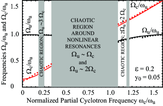
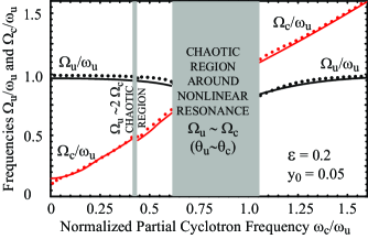
Figure 2: Undulator and cyclotron frequencies vs. the partial cyclotron frequency. The adiabatic undulator entrance of electrons to the interaction region is neglected. Solid lines are for the analytical results, while dots correspond to the results of the numerical simulation.

Figure 3: Undulator and cyclotron frequencies vs. the partial cyclotron frequency. The adiabatic undulator entrance is taken into account.

The comparison of the results for $\Omega_{u}$ and $\Omega_{c}$ obtained by using the analytical expressions (solid lines) and the numerical simulation of Eqs. (15) (dots) is demonstrated in Fig. 3 and 3. For both of the situations the analytical and numerical results are seemed to be in a good agrement. Note that in our analytical study we ignore the adiabatic undulator entrance of electrons to the interaction region. The comparison between Figs. 3 and 3 gives a clear indication that the adiabatic undulator entrance ”improve integrability” of the nonlinear dynamical system (15) and reduce the width of chaotic regions. In Goryashko et al. (2009) it was found that the initial positive value for the $x$-component of the velocity leads to the suppression of the chaotic region. A test electron acquires such a positive average correction to $v_{x}$ passing through the region of the adiabatic entrance. And, as a result, the chaotic dynamics of the electron in the regular undulator region is partially suppressed. A rough analytical estimate indicates that the average correction is about one fourth of the amplitude of $v_{x}$-oscillations in the regular undulator.

III.3 Chaotic motion

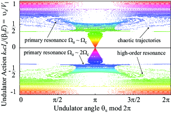
Figure 4: Poincare mapping to the system (15); $\vartheta_{c}=0$.

The equation set (15) has a lot of nonlinear resonances (16) ($n\vartheta_{u}\approx m\vartheta_{c}$) between the undulator and cyclotron degrees of freedom, therefore one can expect the appearance of chaotic dynamics in the system behavior. In Fig. 4 we have demonstrated the Poincare mapping in which the primary and the higher resonances are seen; the separate dots correspond to the stochastic trajectories. Note that the average axial velocity for the majority of the stochastic trajectories equals zero. As evident from Eq. (20) and Eq. (21), the undulator action (integral of motion!) can vanish under some conditions. This means the destruction of the integral motion (Sagdeev et al., 1988, ch. 5) and chaotization of the dynamics of the test electron. Hence, the motion becomes stochastic if the difference between the undulator and cyclotron frequencies becomes less than the betatron frequency

$$|\Omega_{u}-\Omega_{c}|\leq\sqrt{2}\omega_{\beta}\cosh[k_{u}y_{0}]\quad(|\kappa-\sigma|\leq\varepsilon\cosh[k_{u}y_{0}]).$$ (27)

Such a criteria was initially proposed in Goryashko et al. (2009) using some numerical findings. With the derived $\varkappa$ and $\sigma$ we get the expression describing the location of the region of the dynamic chaos:

$$\begin{split}&\sigma_{0}^{crit1}\leq\sigma_{0}\leq\sigma_{0}^{crit2},\\ &\sigma_{0}^{crit2}=\frac{2}{3}+\frac{28\varepsilon\cosh[k_{u}y_{0}]}{27}+\frac{5\varepsilon^{2}\cosh^{2}[k_{u}y_{0}]}{18}.\end{split}$$ (28)

It turns out that the chaotization condition is inconsistent with the solution of equation set (21) for $\varepsilon$ less than the minimal value of $\varepsilon^{min}$

$$\varepsilon^{min}\cosh[k_{u}y_{0}]=0.0786.$$ (29)

In the used approximations this implies that there is no the chaotic region for $\varepsilon<\varepsilon^{min}$.

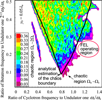
Figure 5: The major Lyapunov exponent map. Black solid lines show the boundaries of the chaotic region according to the analytical formulae (28).

In Fig. 5 we have illustrated the results of the numerical calculations for the major Lyapunov exponent. The solid lines calculated using equation (28) show the boundaries of the chaotic region. They are in a good agreement with the results of numerical simulation.

In what follows we analyze the studied FEL within the region of the regular dynamic.

IV The reduced model of the FEL

In this section we construct the time-dependent reduced FEL model that allows for the complicated dynamics of electrons in the pump magnetic field and intramode scattering in an irregular waveguide. Since we are going to analyze the resonant interaction between the microwave and electron beam we may approximately rewrite vector-potential $A_{x}^{s}$ as (see B)

$$A_{x}^{s}=\mathrm{Re}\Bigl{\{}\bigl{[}V_{+}(z,t)+V_{-}(z,t)\bigr{]}\sqrt{\frac{k_{z}^{0}b}{k_{z}(z)w(z)}}\times\\ \cos\Bigl{(}\frac{\pi y}{w(z)}\Bigr{)}\,e^{-i\omega t+i\Psi(z)}\Bigr{\}}.$$ (30)

Here $\Psi(z)=\int_{0}^{z}k_{z}(z^{\prime})dz^{\prime}$, $V_{+}(z,t)$ and $V_{-}(z,t)$ are the amplitudes of the forward and backward waves governed by the following excitation equations

$$\frac{\partial V_{+}}{\partial z}+\frac{1}{v_{gr}(z)}\frac{\partial V_{+}}{\partial t}=J^{e}(z,t),$$ (31a)

$$\frac{\partial V_{-}}{\partial z}-\frac{1}{v_{gr}(z)}\frac{\partial V_{-}}{\partial t}+2ik_{z}V_{-}=\frac{\partial k_{z}}{\partial z}\frac{V_{+}}{2k_{z}}.$$ (31b)

The Eq. (31a) describes the interaction between the beam and forward wave, whereas the Eq. (31b) describes the scattering of the forward wave to the backward one. The boundary conditions are

$$V_{+}\bigr{|}_{z=0}=V_{0},\quad V_{-}\bigr{|}_{z=L}=0.$$ (32)

The effective current

$$J^{e}(z,t)=\frac{4iI_{0}\omega}{k_{z}^{0}Sc}\sqrt{\frac{k_{z}^{0}b}{k_{z}w}}\frac{1}{Y_{b}}\int\limits_{-Y_{b}/2}^{Y_{b}/2}\!\!dy_{0}\int\limits_{t-t^{p}-\pi/\omega}^{t-t^{p}+\pi/\omega}\!\!dt_{e}\times\\ \frac{p_{x}(z;y_{0},t_{e})}{p_{z}(z;y_{0},t_{e})}\cos\Bigl{(}\frac{\pi y(z;y_{0},t_{e})}{w(z)}\Bigr{)}e^{i\omega t(z;y_{0},t_{e})-i\Psi(z)}$$ (33)

at moment $t$ and position $z$ is generated by the group of electrons entered into the interaction region during the time interval from $(t-t^{p}(z;y_{0})-\pi/\omega)$ to $(t-t^{p}(z;y_{0})+\pi/\omega)$. Here $t^{p}(z;y_{0})$ is the arrival time of the electron, which moves in the pump magnetic field (1), to the cross-section $z$. According to Eq. (3) and Eq. (5) the integrating over $t^{\prime}$ yields a non-zero result only if $t-\pi/\omega\leq t(z;y_{0},t_{e})\leq t+\pi/\omega$ because of the Dirac delta. Since the right-hand side of excitation equation (3) is a slow function of time we may write $t(z;y_{0},t_{e})\approx t_{e}+t^{p}(z;y_{0})$ and find integration limits with respect to $t_{e}$.

In the previous Section we have studied the nonlinear system with the Hamiltonian (9) and found trajectories as functions of actions $\vec{\bar{I}}$ and angles $\vec{\bar{\vartheta}}$. Now let us take into account the ponderomotive potential $W(\vec{r},\vec{P},t)$. We will hold $\bar{\mathcal{H}}(\vec{r},\vec{P})$ as the integrable part of the Hamiltonian (8) and consider the relation (19) between $(\vec{r},\vec{P})$ and $(\vec{\bar{I}},\vec{\bar{\vartheta}})$ as a variable replacement rule, regarding $(\vec{\bar{I}},\vec{\bar{\vartheta}})$ as new unknown variables. The perturbation $W(\vec{\bar{I}},\vec{\bar{\vartheta}},t)$ periodically depends on angles $\bar{\vartheta}_{u}$ and $\bar{\vartheta}_{c}$, therefore it can be represented as a double Fourier-series over $\bar{\vartheta}_{u}$ and $\bar{\vartheta}_{c}$: $W\propto W_{n,m}e^{-i\omega t+i\Psi(\bar{\vartheta}_{u})+in\bar{\vartheta}_{u}+im\bar{\vartheta}_{u}}$ ($m$ and $n$ are integers). As we have already known from Sec. III the slower is phase changing $\omega t-\Psi-n\bar{\vartheta}_{u}-m\bar{\vartheta}_{u}$, the stronger is the action of Fourier-component $W_{n,m}$ (see text below Eq. (15)). The main principle of the nonlinear resonance analysis is simple (Sagdeev et al., 1988, ch. 3): the ‘troublesome’ resonant term is separately extracted from the perturbation expansion and, in the sequel, the dynamics caused by this term is studied. Further on, we analyze the undulator resonance

$$\bar{\vartheta}_{u}+\int_{0}^{\bar{\vartheta}_{u}/k_{u}}k_{z}(z^{\prime})dz^{\prime}\approx\omega t\quad((k_{z}+k_{u})\bar{v}_{\|}\approx\omega).$$ (34)

and may write the ponderomotive perturbation as

$$W(\vec{\bar{I}},\vec{\bar{\vartheta}},t)\approx\mathrm{Re}\bigl{\{}\tilde{W}(\bar{I}_{u},z(\bar{\vartheta}_{u}),t)e^{i\psi(\bar{\vartheta}_{u},t)}\bigr{\}},$$

where

$$\tilde{W}=-ec\,\frac{\varepsilon p_{\|}\Delta_{u}^{2}\cosh[k_{u}y_{0}]}{\Delta_{u}^{2}-\sigma_{0}^{2}}\bigl{(}V_{+}+V_{-}\bigr{)}\sqrt{\frac{k_{z}^{0}b}{k_{z}w}}\cos\Bigl{(}\frac{\pi y}{w}\Bigr{)}.$$

Quantity $\tilde{W}(\bar{I}_{u},z(\bar{\vartheta}_{u}),t)$ is a slow function of $\bar{\vartheta}_{u}$ and $t$ via a slow variation of the waveguide profile and the microwave amplitude. The equations of motion is

$$\begin{split}\dot{\bar{I}}_{u}&=-\frac{1}{2\mathcal{H}}\frac{\partial W}{\partial\bar{\vartheta}_{u}}\quad\dot{\bar{\vartheta}}_{u}=\frac{\mathcal{E}}{\mathcal{H}}\;\Omega_{u}(\vec{\bar{I}})+\frac{1}{2\mathcal{H}}\frac{\partial W}{\partial\bar{I}_{u}},\\ \dot{\bar{I}}_{c}&=0,\qquad\quad\dot{\bar{\vartheta}}_{c}=\Omega_{c}(\vec{\bar{I}})\;\mathcal{E}/\mathcal{H}.\end{split}$$ (35)

To obtain the equations of motion in the simplest form and clearly demonstrate the physics of FELs with the axial magnetic field we additionally suppose that $\mathcal{H}-\mathcal{E}\ll\mathcal{E}$ (‘Compton limit’). Applying the method of the nonlinear resonance (Sagdeev et al., 1988, ch. 3) to Eqs. (35), using $z$ as a new independent variable and defining the ponderomotive phase as $\psi=k_{u}z+\int_{0}^{z}k_{z}(z^{\prime})dz^{\prime}-\omega t$, we get the equation for $\psi$

$$\frac{\partial^{2}\psi}{\partial z^{2}}-\frac{\partial k_{z}}{\partial z}=-\frac{1}{\bar{v}_{\|}^{2}}\frac{\omega}{\Omega_{u}}\Bigl{(}1+\frac{k_{z}}{k_{u}}\Bigr{)}\frac{1}{2\mathcal{H}}\frac{\partial W}{\partial\psi}\frac{\partial}{\partial{\bar{I}_{u}}}\Bigl{[}\frac{\mathcal{E}}{\mathcal{H}}\;\Omega_{u}\Bigr{]},$$

where the derivative of the undulator frequency is

$$\frac{\partial}{\partial{\bar{I}_{u}}}\Bigl{[}\frac{\mathcal{E}}{\mathcal{H}}\;\Omega_{u}\Bigr{]}\approx\frac{\omega_{u}\mathcal{E}}{I_{u}^{0}}\frac{\partial}{\partial{\bar{I}_{u}}}\frac{{\bar{I}_{u}}}{\mathcal{H}}\approx\frac{\omega_{u}^{2}}{\beta_{\|}^{2}\bar{\gamma}_{\|}^{2}\mathcal{E}}\quad\Bigl{(}\frac{1}{\bar{\gamma}_{\|}^{2}}=1-\frac{\bar{v}_{\|}^{2}}{c^{2}}\Bigr{)}.$$

Expanding the ponderomotive current into a series with respect to angles and taking into account only the resonant term in the excitation equation one can write the reduced FEL model in the following manner:

$$\begin{split}&\frac{\partial^{2}\tilde{\psi}}{\partial\zeta^{2}}=-Y(y_{0})Z(\zeta)\;\mathrm{Re}\{\bigl{(}F_{+}+F_{-}\bigr{)}e^{i\tilde{\psi}}\},\\ &\frac{\partial F_{+}}{\partial\zeta}-i\delta_{z}(\zeta)F_{+}+\Bigl{(}\frac{\bar{v}_{\|}}{v_{gr}}-1\Bigr{)}\frac{\partial F_{+}}{\partial\tau}=\tilde{J}^{e}(\zeta,\tau),\\ &\frac{\partial F_{-}}{\partial\zeta}+i(2k_{z}\ell_{g}-\delta_{z})F_{-}-\Bigl{(}1+\frac{\bar{v}_{\|}}{v_{gr}}\Bigr{)}\frac{\partial F_{-}}{\partial\tau}=\frac{\partial k_{z}}{\partial\zeta}\frac{F_{+}}{2k_{z}},\\ &\tilde{J}^{e}(\zeta,\tau)=\frac{Z(\zeta)}{\pi Y_{b}}\!\!\int\limits_{-Y_{b}/2}^{Y_{b}/2}\!\!dy^{\prime}_{0}\!\!\int\limits_{-\pi}^{\pi}\!\!d\psi^{\prime}_{0}\,Y(y^{\prime}_{0})e^{-i\tilde{\psi}(\zeta,\tau;y^{\prime}_{0},\psi^{\prime}_{0})},\\ &\tilde{\psi}|_{\zeta=0}=\psi_{0},\quad\frac{\partial\tilde{\psi}}{\partial\zeta}\Bigr{|}_{\zeta=0}\equiv\delta_{y}(y_{0})=\frac{\ell_{g}\omega}{\bar{v}_{\|}(0)}-\frac{\ell_{g}\omega}{\bar{v}_{\|}(y_{0})},\\ &F_{+}\Bigr{|}_{\zeta=0}=F_{0},\quad F_{-}\Bigr{|}_{\zeta=L/\ell_{g}}=0.\end{split}$$ (36)

Here $\zeta=z/\ell_{g}$ and $\tau=(\bar{v}_{\|}t-z)/\ell_{g}$ are the dimensionless longitudinal coordinate and ”retarded time”  Bonifacio et al. (1992);

$$F_{\pm}=-\frac{iec\omega^{2}\ell_{g}^{2}}{\sqrt{2}\bar{v}_{\|}^{3}\bar{\gamma}_{\|}^{2}\mathcal{E}}\frac{\omega_{\beta}}{\Omega_{u}}\,V_{\pm}\,e^{i\int_{0}^{\zeta}\delta_{z}(\zeta^{\prime})d\zeta^{\prime}}$$ (37)

is the normalized field amplitude; $\tilde{\psi}(\zeta,\tau;y_{0},\psi_{0})=\psi(\zeta,\tau;y_{0},\psi_{0})-\int_{0}^{\zeta}\delta_{z}(\zeta^{\prime})d\zeta^{\prime}$ is the ponderomotive phase; $\psi_{0}$ and $y_{0}$ are the initial entrance phase and the initial transverse displacement of the electron’s position from the undulator symmetry plane $y=0$;

$$\ell_{g}^{-3}=\frac{1}{\bar{\beta}_{\|}^{3}\bar{\gamma}_{\|}^{3}}\frac{I_{0}}{I_{\alpha}}\frac{2\pi\omega^{2}}{k_{z}^{0}Sc^{2}}\frac{\omega_{\beta}^{2}}{\Omega_{u}^{2}},$$ (38)

where $I_{\alpha}=m_{e}c^{3}/e\approx-17$ kA is the Alfvén current (recall that $e,I_{0}<0$). The parameter $\ell_{g}$ is called the gain length Bonifacio et al. (1992) (the spatial growth rate of the FEL without the axial magnetic field is equal to $\ell_{g}^{-1}$ for zero detuning). The explicit dependence of the reduced FEL model on the transverse electron’s position and the axial position are given by the relations

$$Y=\frac{\Omega_{u}^{2}(y_{0})\cosh[k_{u}y_{0}]}{\Omega_{u}^{2}(y_{0})-\Omega_{c}^{2}(y_{0})}\cos\Bigl{[}\frac{\pi y_{0}}{w(z)}\Bigr{]},\;Z=\sqrt{\frac{k_{z}^{0}b}{k_{z}(z)w(z)}}.$$

The dimensionless detuning parameter is

$$\delta_{z}(\zeta)=\ell_{g}\Bigl{(}k_{z}(\zeta)+k_{u}-\frac{\omega}{{\bar{v}_{\|}}(0)}\Bigr{)}.$$ (39)

Note that our model includes two detuning parameters: $\delta_{z}(\zeta)$ changing along the interaction region and $\delta_{y}(y_{0})$ changing across the beam. The physical meaning of these parameters is discussed in detail below.

The time-dependent model (36) allows for the intricate dynamics of electrons in the pump magnetic field (1), the effect of the electron beam finite thickness and the intramode scattering in the profiled waveguide (the intramode scattering acts actually as a feedback). Our model (36) is exactly coincident with the Colson-Bohifacio model Colson (1976); Bonifacio et al. (1984) if a free-space case is employed, the axial magnetic field equals zero, the electron beam is ideally thin and ultrarelativistic. In the above case, the field amplitude $F_{+}$ depends mainly on detuning parameter $\delta_{z}$ if the initial value of $F_{+}$ is sufficiently small. Then the FEL operates efficiently if $|\delta_{z}|<2$ (see Fig. 2 in Bonifacio et al. (1992); Barré et al. (2004)). Otherwise, our model (36) is dependent upon more than one parameter and incorporates some novel effects. It is worth noting that using the method of nonlinear resonance in the action-angle phase space one can reduce any Hamiltonian with the resonant perturbation to the so-called Universal Hamiltonian of nonlinear resonance (Sagdeev et al., 1988, ch. 3). This means that any resonant beam-wave interaction can be described within the framework of the reduced model that includes the pendulum-like equations of motion of electrons and the excitation equation of Colson-Bonifacio type. The equations of motion have dimensions of one and a half. In our case, the beam-wave energy transfer occurs through the undulator degree of freedom only, whereas the energy stored in the cyclotron degree remains unchanged.

What is important is that the model (36) depends solely on the average axial velocity via the detuning but does not depend on the particular scalar components of the initial velocity. This results in that the FEL efficiency is only dictated by the spread of the average axial velocity such that $\delta\bar{v}_{\|}\propto\delta v_{z}+\varepsilon\delta v_{x}+\varepsilon^{2}\delta v_{y}$, where $\delta v_{i}(t_{e})$ $(i=x,y,z)$ is the magnitude of the initial velocity spread ($\delta v_{i}/\bar{v}_{\|}\ll 1$) and $\delta\bar{v}_{\|}(t_{e})$ is the average axial velocity spread. Recall that $\varepsilon=\sqrt{2}\omega_{\beta}/\omega_{u}$ is a small parameter. It is clear that one first needs to minimize the initial axial velocity spread. The analysis of the FEL indicates that the velocity spread changes the efficiency insignificantly if the detuning caused by the spread is much smaller than unity Bonifacio et al. (1992). For the ideally thin beam ($Y_{b}\rightarrow 0$) it yields the condition

$$\frac{(k_{z}^{0}+k_{u})\ell_{g}}{Y^{2/3}}\frac{\mu_{\bar{v}_{\|}}}{\bar{v}_{\|}}\ll 1,$$ (40)

where $\mu_{\bar{v}_{\|}}$ is the variance of $\delta\bar{v}_{\|}$. It was shown in Freund and Ganguly (1986b) (see also the results of the numerical simulation in Goryashko et al. (2009)) that essential decreases in the sensitivity of the the efficiency to the initial beam spread can be obtained if the undulator frequency is close to the cyclotron one (multiplier $Y^{-2/3}$ attains its minimal value).

In general, the ponderomotive potential enhances as the undulator frequency tends to the cyclotron one ($Y(y_{0})$ increases). This results in a stronger coupling between the wave and electrons. Such an effect referred to as the magnetoresonance is well-known in the literature Sprangle and Granatstein (1978) and the recent detailed study Goryashko et al. (2009) confirmed the usefulness of such a regime for a planar FEL configuration. However, the magnetoresonance effect is not so effective when the beam has a finite thickness. Electrons with the different initial transverse positions, $y_{0}$, undergo the action of the different magnitudes of the pump magnetic field (1). Then the average velocity of the electron depends on its initial transverse positions $y_{0}$ (this dependence particulary strong near the magnetoresonance). At the same time the average velocity of the electron of the beam governs the initial ‘transverse’ detuning $\delta_{y}(y_{0})$ between the electron and the wave. Hence, the value of $\delta_{y}(y_{0})$ changes across the beam, and the contribution of different electrons to the total efficiency might be quite different. To demonstrate this effect we simulate Eqs. (36) for the parameters close to the experiment Cheng et al. (1996) and assume there is additional axial magnetic field 20 kG as well.

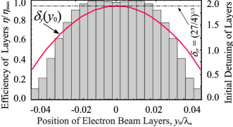
Figure 6: The relative efficiency (histogram) and the initial detuning (red solid line) of electron beam layers vs. the normalized transverse displacement of layers from the symmetry plane $y=0$.

In the simulation we split the beam into 21 layers in the transverse cross-section. Each layer is also uniformly distributed into 50 macroparticles entering within one wave period. Recall that the physical system under study is homogenous in the $x$-direction. The results are shown in Fig. 6. The internal layer operates in the regime of optimal (with respect to efficiency) detuning $\delta_{z}(\zeta)=\delta_{cr}=(27/4)^{1/3}$ and $\delta_{y}\equiv 0$ but the external layers operate with the non-optimal detuning because of the variation in $\delta_{y}$ (illustrated in Fig. 6 as the solid line) across the beam.

It should be anew mentioned that under certain conditions the integral of motion of a typical electron fails and dynamics becomes chaotic. Now we can derive the chaotization condition including the effect of the microwave. In the microwave saturation region one can hold the average value of the undulator action as an integral of motion, then the condition $\langle I_{u}\rangle>0$ has to be fulfiled to preserve the regular dynamics of electrons and the validity of model (36). In the case of the steady-state regime, when the beam is thin and the waveguide is regular, the improved chaotization condition is

$$\frac{2\omega_{\beta}^{2}}{(\Omega_{u}-\Omega_{c})^{2}}+\frac{\bar{\gamma}_{\|}^{2}\Omega_{u}}{\omega}\frac{|F_{+}|^{2}}{8k_{u}\ell_{g}}\Bigl{|}\frac{\Omega_{u}}{\Omega_{u}-\Omega_{c}}\Bigr{|}^{2/3}<1.$$ (41)

Here we have considered that the microwave field modifies the undulator action by the additional quantity

$$\Delta I_{u}=\frac{\dot{\tilde{\psi}}\Omega_{u}}{\omega}\Bigl{(}\frac{\partial\Omega_{u}}{\partial\bar{I}_{u}}\Bigr{)}^{-1}.$$

Besides, we used the constant of the motion to the Colson-Bonifacio model Gluckstern et al. (1993)

$$\langle\frac{d\tilde{\psi}}{d\zeta}\rangle=-\frac{|F_{+}|^{2}-|F_{0}|^{2}}{4}.$$

It is obvious from Eq. (41) that the microwave may cause the chaotization of electrons even if the dynamics was regular in the pure pump field.

Another important feature of the model (36) is that it takes into account the effect of waveguide profiling. This effect exhibits the coupling between the forward and backward waves because of intramode scattering as well as the dependence of the wave number, $k_{z}$, on the axial position $z$ through the varying waveguide width, $w(z)$. As a result, the detuning $\delta_{z}$ is also a function of the axial position and its control can be used to govern the beam-wave interaction.

V Control of the beam-wave interaction: FEL with the
optimized waveguide profile

Now discuss the physical principle of the control of the beam-wave interaction. For simplicity we consider the steady-state regime and the thin beam. We also neglect the backward wave generation assuming that $w(z)$ is a slow function of $z$. Rewriting the complex amplitudes of the wave and ponderomotive current as $F_{+}=|F_{+}|e^{i\alpha}$ and $\tilde{J}^{e}=|\tilde{J}^{e}|e^{iu_{\ast}}$ and using Eqs. (36) we arrive at the system:

$$\begin{split}&\frac{d^{2}\tilde{\psi}}{d\zeta^{2}}=-|F_{+}|\cos(\alpha+\tilde{\psi}),\quad\frac{d|F_{+}|}{d\zeta}=|\tilde{J}^{e}|\cos(\alpha-u_{\ast}),\\ &\frac{d\alpha}{d\zeta}=\delta_{z}\bigr{(}\zeta)-|\tilde{J}^{e}|\sin(\alpha-u_{\ast})/|F_{+}|.\\ &u_{\ast}=\mathrm{Arg}\Bigl{(}\frac{1}{\pi}\int_{0}^{2\pi}\!\!\!e^{-i\tilde{\psi}}\,d\psi_{0}\Bigr{)},\quad|\tilde{J}^{e}|=\frac{1}{\pi}\Bigl{|}\int_{0}^{2\pi}\!\!\!e^{-i\tilde{\psi}}\,d\psi_{0}\Bigr{|}.\end{split}$$ (42)

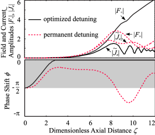
Figure 7: The simulation results for the FEL with and without the phase shift optimization are demonstrated.

Here $\tilde{\psi}$, $|F_{+}|$ and $\alpha$ are the unknown quantities governed by the differential equations, and $u_{\ast}$ and $|\tilde{J}^{e}|$ are given by definition. The phase of the current $u_{\ast}$ defines the position of the bunch center in the system of coordinates moving with the velocity of the beam (Vainshtein and Solntsev, 1973, p. 160) (see also (Tsimring, 2007, p. 325)). One can see that if the phase shift between the current and the wave, $\phi=\alpha-u_{\ast}$, belongs to the interval from $-\pi/2$ to $\pi/2$, then the right-hand side of the equation governing wave amplitude $|F_{+}|$ (second equation in the upper line of (42)) has a positive sign and the amplitude itself grows. The phase shift $\phi$ governs the energy transfer from the beam to the wave (or v.v.) because the local interaction power is $dP/d\zeta\propto|\tilde{J}^{e}||F_{+}|\cos\phi$. This implies that we can increase the efficiency by controlling $\phi$ along the interaction region by changing the detuning parameter $\delta_{z}(\zeta)$ in an appropriate way. The idea of such an optimization was originally proposed in the TWT theory Solnzev (1971). Here, for example, we demonstrate the simple indirect optimization method Solnzev (1971). Now assume that the phase shift, $\phi$, satisfies the relation:

$$\begin{split}\alpha-u_{\ast}\equiv\phi_{opt}(\zeta)&=-\pi\sin^{2}\frac{\pi\zeta}{2L_{pr}},\quad\zeta\leq L_{pr},\\ \alpha-u_{\ast}\equiv\phi_{opt}(\zeta)&=0,\qquad\qquad\qquad\zeta>L_{pr},\end{split}$$ (43)

where $L_{pr}$ is the start point of the region with the permanent value of $\phi$. Then we have to find $\tilde{\psi}$ and $|F_{+}|$ using Eqs. (42) and Eq. (43) (in the right-hand sides of Eqs. (42) the expression $(\alpha-u_{\ast})$ should be replaced by $\phi_{opt}$). Now we can restore the information about the waveguide profile using the equation for the detuning parameter that follows from (42):

$$\delta_{z}\bigr{(}\zeta)=\frac{du_{\ast}}{d\zeta}+\frac{d\phi_{opt}}{d\zeta}+(|\tilde{J}^{e}|\sin\phi_{opt})/|F_{+}|.$$ (44)

The results from the calculation of the amplitudes of the wave $|F_{+}|$ and the current $|\tilde{J}^{e}|$, and the phase shift $\phi$ are shown in Fig. 7. In this figure we also plotted the FEL characteristics for the constant detuning. We can see that the wave amplitude can be significantly enhanced (efficiency increased several times). However, the demonstrated optimization technique is useful only for a slightly improved efficiency because the waveguide profiles are to be rather complicated from the practical point of view in an effort to considerably increase the efficiency. Then more elaborated mathematical approaches, which simultaneously allow one to control the practical realizability of optimal waveguide profiles, should be used. In this paper we apply some type of a genetic algorithm Mitchell (1999) to perform the FEL optimization. The principle of evolutionary optimization is rather simple: we generate a lot of waveguide profiles and then perform numerical simulation of the reduced model (36) using these profiles. Then we choose the best profiles, cross and modify them, and perform the simulation again. As a result one can find a few best profiles. Finally we must check that these found optimal profiles are really useful. We have to simulate the non-simplified original model (formulated in Sec. II) using these profiles. Let us consider the results of the optimization for a practical example.

The FEL parameters are chosen to be close to the parameters of experiment Cheng et al. (1996): 450-kV beam voltage, $|I_{0}|=16$-A beam current, 1.0 mm $\times$ 2.0 cm sheet electron beam interacts with the TE₀₁ mode (the field varying along the narrow wall) of the 4.5 mm $\times$ 4.0 cm rectangular waveguide. The undulator magnitude increases adiabatically within six periods and the undulator is characterized by parameters $B_{u}=3.5$ kG and $\lambda_{u}=1.0$ cm in the regular region. A 1-kW input signal with the 4.0 mm wavelength is injected. In our simulation we assume that there is the axial magnetic field 20 kG as well. The wavelength is slightly different from that in the experiment because of the different average axial velocity. In Fig. 8A the results for the FEL with the axial field but without optimization are shown. Using the magnetoresonance effect we can significantly enhance the efficiency. It was 4% efficiency without the axial field in the experiment and it is 12% efficiency with the axial magnetic field. However, there is a weak interaction between the external beam layers and the microwave because different layers of the electron beam have different ”transverse” detuning with the wave due to the transverse inhomogeneity of the pump magnetic field. Geometric positions of different beam layers at the beginning of the interaction region are shown inside the dotted ellipse. The black curve is for the central layer. Other layers are displaced with respect to the symmetry plane $y=0$.

In Fig. 8B the results for the optimized FEL with the axial field are presented. Using the waveguide with the optimized profile one can double the efficiency so that the final efficiency is around 22%. We also see the external layers interact with the wave much more effectively in the optimized FEL. So, by changing the waveguide profile we control beam-wave interaction thus increasing the FEL efficiency.

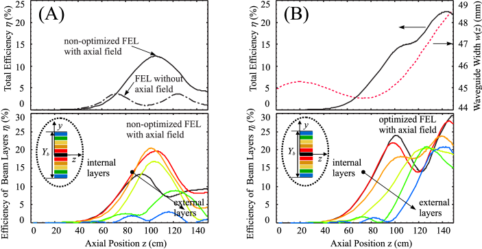
Figure 8: The FEL efficiency and waveguide width vs. the interaction length. The results of the non-simplified model simulation are demonstrated.

VI Summary and Discussion

The operation of the planar FEL-amplifier with the axial magnetic field and the irregular waveguide is studied. The self-consistent model, which includes the excitation equation and the equations of motion along with the expressions for the radiated field and the microscopic current density, is formulated. In order to find the parameters and the waveguide profile that provides the maximal efficiency one has to perform some optimization of the FEL. However, the conventional numerical optimization methods fail to work because a vast amount of computational resources is required. Typically, about several thousand equations of motions and the partial differential equation for the wave amplitude have to be simulated. In this paper I propose another approach to the problem. The investigation is divided into several stages: initially I partly integrate equations of motion and the excitation equation in an analytical way using methods of nonlinear dynamics. As a result, the universal reduced FEL model is derived in special phase space. Then with this model and some principles of evolutionary computations (genetic algorithms) I perform the numerical optimization of the waveguide profile. Finally, the simulation of the non-simplified original model using the found optimal waveguide profiles is carried out. So, one can come closer to understanding of what increase in the efficiency can be achieved in practise.

To derive the reduce model one first can find the integrals of motion of a test electron in the pump magnetic field (1) applying the overconvergent method. The dynamics is completely governed by the two integrals of motion corresponding to the undulator and cyclotron degrees of freedom. At the same time it is reasonable to use other two parameters that completely define the dynamics as well: the first governing parameter $\varepsilon=\sqrt{2}\omega_{\beta}\cosh[k_{u}y_{0}]/\omega_{u}$ is the level of nonlinearity and the second one $\sigma_{0}=\omega_{c}/\omega_{u}$ shows how the system is close to the magnetoresonance. The complete description of the dynamics is given in terms of these parameters. It is well known that the dynamics in the pump field is chaotic for some parameters Michel-Lours et al. (1993), so the explicit expression (28) describing the region location of the dynamic chaos in the parameter space ($\varepsilon,\sigma_{0}$) are derived and the existence domain of integrals of motion is formulated. From the plot of the Lyapunov exponent we see that analytical formulae (28) give an accurate definitions of the chaotic zone boundaries. Note that the afore-mentioned technique can also be applied to the pure undulator field (there is no the axial field). In this case from Eq. (27) it follows a simple chaotization condition that in terms of paper Chen and Davidson (1990) reads

$$a_{w}\geq\beta_{zb}\gamma_{b}/(\sqrt{2}\cosh[k_{w}x_{b}]).$$ (45)

In Fig. 9 the regular and chaotic regions in the parameter space $(k_{w}x_{b},a_{w})$, according to Eq. (45), are shown. Comparing Fig. 2 of Chen and Davidson (1990) and Fig. 9 of the present paper we notice that the proposed simple estimation is in a reasonable agreement with the numerical simulation result cited in paper Chen and Davidson (1990).

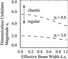
Figure 9: The boundaries of regular and chaotic regions obtained using Eq. (45) (cf. with Fig. 2 in Chen and Davidson (1990)).

Using the information about the electron’s dynamics in the pump magnetic field one can subsequently analyze the dynamics of ensemble of electrons in view of the ponderomotive wave. In a special coordinate system (that moves on the invariant torus surface if there is no the ponderomotive wave) one can split degrees of freedom and partially integrate the equations of motion Sagdeev et al. (1988). As a result, the universal reduced model of the FEL (36) that incorporates the intricate dynamics of electrons and the intramode scattering is derived.

What is important is that there are two types of detuning in reduce model (36): ‘axial’ detuning that changes along the interaction region via the profiled waveguide width and the ‘transverse’ detuning that changes across the beam because the pump magnetic field is inhomogeneous and the average velocity of the electron depends on its initial transverse position. The ”transverse” detuning causes the thick beam layering and the degradation of the external layers’ contribution into the total efficiency (the degradation is particulary strong near the magnetoresonance). In the present paper I demonstrate that this problem and the saturation effect can be overcome by the control of the beam-wave interaction. The physical mechanism of such a control is that by changing the waveguide profile one control the axial detuning and thus regulate the phase shift between the ponderomotive wave and current. This phase shift defines the transfer of the energy between the beam and the wave and its regulation allows one to optimize the interaction.

The practical example of optimization of the FEL, whose parameters are close to those of the experiment Cheng et al. (1996), is demonstrated. The simulation results based on the non-simplified model (see Sec. II) strongly indicate that combining the magnetoresonance effect with the optimized profile waveguide one can enhance the FEL efficiency by a factor of five or six. The efficiency in the experiment Cheng et al. (1996) was around 4%. Applying the axial magnetic field the efficiency has been increased up to nearly 12%, but about 30% of electrons do not interact with the wave because of the initial transverse detuning. Following the waveguide optimization the efficiency has reached 22%, in particular, due to a much more effective interaction between the external beam layers and the wave.

Appendix A Time-dependent excitation equation of an irregular waveguide

The evolution of the resonant (synchronous) TE₀₁ mode is governed by the $x$-component of the vector-potential $A_{x}^{s}$, which satisfies the wave equation

$$g\Bigl{(}\nabla^{2}-\frac{1}{c^{2}}\frac{\partial^{2}}{\partial t^{2}}\Bigr{)}A_{x}=-\frac{4\pi}{c}j_{x}.$$ (46)

We seek a solution to the equation of the form:

$$A_{x}(\vec{r},t)=\mathrm{Re}\int_{0}^{\infty}\bar{V}_{(}z,\omega^{\prime})\sqrt{\frac{b}{w(z)}}\cos\Bigl{(}\frac{\pi y}{w(z)}\Bigr{)}\,e^{-i\omega^{\prime}t}\,d\omega^{\prime}.$$ (47)

Substituting (47) into (46) we derive the excitation equation for the Fourier amplitude $\bar{V}_{(}z,\omega^{\prime})$

$$\Bigl{\{}\frac{\partial^{2}}{\partial z^{2}}+k_{z}^{2}(z,\omega^{\prime})\Bigl{\}}\bar{V}_{(}z,\omega^{\prime})=-\frac{8\pi}{Sc}\sqrt{\frac{b}{w(z)}}\int_{-a/2}^{a/2}dx\times\\ \int_{-w/2}^{w/2}dy\,\bar{j}_{x}(\vec{r},\omega^{\prime})\cos\Bigl{(}\frac{\pi y}{w(z)}\Bigr{)},$$ (48)

where $k_{z}^{2}(z)=(\omega/c)^{2}-(\pi/w)^{2}-(w^{\prime}/2w)^{2}(1+\pi^{2}/3)$ and $\bar{j}_{x}(\vec{r},\omega^{\prime})=\pi^{-1}\int_{-\infty}^{\infty}j_{x}(\vec{r},t)e^{i\omega^{\prime}t}dt$. Here $\bar{j}_{x}(\vec{r},\omega^{\prime})$ is the Fourier amplitude of the current density. We will consider that at the section $z=0$ the FEL-amplifier is seeded by the TE₀₁ mode with a frequency of $\omega$ and amplitude $V_{0}$, and the interaction region is ideally matched to a regular output waveguide at the section $z=L$

$$\begin{split}&\Bigl{(}\frac{\partial\bar{V}}{\partial z}+ik_{z}\bar{V}\Bigr{)}\Bigr{|}_{z=0}=2ik_{z}V_{0}\delta[\omega^{\prime}-\omega],\\ &\Bigl{(}\frac{\partial\bar{V}}{\partial z}-ik_{z}\bar{V}\Bigr{)}\Bigr{|}_{z=L}=0.\end{split}$$ (49)

The conditions for the waveguide profile at the ends of the interaction region have the following form: $w^{\prime}(0)=w^{\prime}(L)=0$. We assume that $\bar{j}_{x}(\vec{r},\omega^{\prime})$ is the narrow-band signal with a fundamental frequency of $\omega$. This means that the current density can be written as $j_{x}(\vec{r},t)=\mathrm{Re}\{J_{x}(\vec{r},t)e^{-i\omega t}\},$ where $J_{x}(\vec{r},t)$ is a slow function of time such that

$$J_{x}(\vec{r},t)\approx\frac{\omega}{\pi}\int_{t-\pi/\omega}^{t+\pi/\omega}j_{x}(\vec{r},t)e^{i\omega t}dt\approx\\ \int_{-\infty}^{\infty}\bar{j}_{x}(\vec{r},\omega+\Delta\omega)e^{-i\Delta\omega t}d(\Delta\omega),\quad\Delta\omega=\omega^{\prime}-\omega.$$

Expanding $k_{z}^{2}(z,\omega^{\prime})$ into Taylor’s series over $\omega$ up to the linear term, multiplying the Eq. (48) by $e^{-i\Delta\omega t}$ and integrating it over $\Delta\omega$ from $-\infty$ to $\infty$ we derive the time-dependent excitation equation (3) for the slow in time amplitude $V(z,t)=\int_{-\infty}^{\infty}\bar{V}(z,\omega+\Delta\omega)e^{-i\Delta\omega t}d(\Delta\omega)$. The solution (47) and the boundary conditions (49) can be rewritten as Eq. (2) and Eq. (4), respectively.

Appendix B Intramode scattering in an irregular waveguide

The Eq. (3) is used for the numerical simulation of non-averaged model of the FEL, but for the analytical study we have to rederive the excitation equation in a different form. We seek a solution to Eq. (48) for microwave Fourier amplitude $\bar{V}$ of the form:

$$\bar{V}=\Bigl{(}\bar{V}_{+}e^{i\Psi}+\bar{V}_{-}e^{-i\Psi}\Bigr{)}\Bigl{(}\frac{k_{z}^{0}}{k_{z}}\Bigr{)}^{1/2},\;\Psi(z)=\int_{0}^{z}k_{z}(z^{\prime})dz^{\prime},$$ (50)

($k_{z}^{0}\equiv k_{z}(0)$) and we allow amplitudes $\bar{V}_{\pm}$ to be functions of the axial position $z$. Applying the method of variation of constants we derive first-order equations for new unknown functions $\bar{V}_{\pm}(z)$

$$\frac{d\bar{V}_{+}}{dz} =-\frac{i\,RHS\,e^{-i\Psi}}{2\sqrt{k_{z}^{0}k_{z}}}+\frac{\partial k_{z}}{\partial z}\frac{\bar{V}_{-}\,e^{-2i\Psi}}{2k_{z}}$$ (51a)

$$\frac{d\bar{V}_{-}}{dz} =\frac{i\,RHS\,e^{i\Psi}}{2\sqrt{k_{z}^{0}k_{z}}}+\frac{\partial k_{z}}{\partial z}\frac{\bar{V}_{+}\,e^{2i\Psi}}{2k_{z}}.$$ (51b)

Here $RHS(z)$ is the right-hand side of Eq. (48) and the boundary conditions become

$$\bar{V}_{+}\bigr{|}_{z=0}=V_{0}\delta[\omega^{\prime}-\omega],\quad\bar{V}_{-}\bigr{|}_{z=L}=0.$$ (52)

Note that Eqs. (50), (51), (52) formally define the exact solution to Eq. (48). Now restrict ourself to the case of the resonant interaction of a beam with a forward microwave. The first term in the right-hand side of (51a) describes the above-mentioned resonant interaction and should be taken into account, whereas the first term in the right-hand side of (51b) is nonresonant and might be omitted. We will also assume that $k_{z}^{-1}\partial_{z}k_{z}<1$ and neglect the second term in the right-hand side of (51a) because it describes the second-order scattering effect (according to the boundary conditions for a source-free regular waveguide $\bar{V}_{-}(z)\equiv 0$), but we will keep the second term in (51b). Using some algebra and performing the inverse Fourier transformation we derive Eqs. (30) and (31) for $V_{+}(z,t)=\int_{-\infty}^{\infty}\bar{V}_{+}(z,\omega+\Delta\omega)e^{-i\Delta\omega t+i\Delta\omega\partial_{\omega}\Psi}d(\Delta\omega)$ and $V_{-}(z,t)=e^{-2i\Psi}\int_{-\infty}^{\infty}\bar{V}_{-}(z,\omega+\Delta\omega)e^{-i\Delta\omega t-i\Delta\omega\partial_{\omega}\Psi}d(\Delta\omega)$.

References

- Ginzburg et al. (2000) N. S. Ginzburg, A. A. Kaminsky, A. K. Kaminsky, N. Y. Peskov, S. N. Sedykh, A. P. Sergeev, and A. S. Sergeev, Phys. Rev. Lett. 84, 3574 (2000).
- Sirigiri et al. (2001) J. R. Sirigiri, K. E. Kreischer, J. Machuzak, I. Mastovsky, M. A. Shapiro, and R. J. Temkin, Phys. Rev. Lett. 86, 5628 (2001).
- Kravchenko et al. (2007) V. F. Kravchenko, A. A. Kuraev, and A. K. Sinitsyn, Physics-Uspekhi 50, 489 (2007).
- Bratman et al. (1983) V. L. Bratman, G. G. Denisov, N. S. Ginzburg, and M. I. Petelin, IEEE J. Quantum Electron. QE-19, 282 (1983).
- Sprangle and Granatstein (1978) P. Sprangle and V. L. Granatstein, Phys. Rev. A 17, 1792 (1978).
- Vainshtein and Solntsev (1973) L. A. Vainshtein and V. A. Solntsev, Lectures on high-frequency electronics (Soviet Radio, Moscow, USSR, 1973), (in Russian).
- Davidson (2001) R. C. Davidson, Physics of Nonneutral Plasmas (Imperial College Press, London, UK, 2001).
- Kroll et al. (1981) N. Kroll, P. Morton, and M. Rosenbluth, IEEE J. Quantum Electron. 17, 1436 (1981).
- Freund and Gold (1984) H. P. Freund and S. H. Gold, Phys. Rev. Lett. 52, 926 (1984).
- Orzechowski et al. (1986) T. J. Orzechowski, B. R. Anderson, J. C. Clark, W. M. Fawley, A. C. Paul, D. Prosnitz, E. T. Scharlemann, S. M. Yarema, D. B. Hopkins, A. M. Sessler, et al., Phys. Rev. Lett. 57, 2172 (1986).
- Freund and Ganguly (1986a) H. P. Freund and A. K. Ganguly, Phys. Rev. A 33, 1060 (1986a).
- Freund and Antonsen (1995) H. P. Freund and T. M. Antonsen, Principles of Free-Electron Lasers (Chapman & Hall, New York, USA, 1995).
- Sinitsky et al. (2009) S. L. Sinitsky, A. V. Arzhannikov, V. T. Astrelin, P. V. Kalinin, and V. D. Stepanov, IEEE Trans. on Plasma Science 37, 1885 (2009).
- Booske et al. (1994) J. H. Booske, M. A. Basten, A. H. Kumbasar, T. M. Antonsen, S. W. Bidwell, Y. Carmel, W. W. Destler, and V. L. Granatstein, Phys. Plasmas 1, 1714 (1994).
- Freund et al. (1987) H. P. Freund, H. Bluem, and C. L. Chang, Phys. Rev. A 36, 2182 (1987).
- Makarov and Tarasov (2001) N. M. Makarov and Y. V. Tarasov, Phys. Rev. B 64, 235306 (2001).
- Goryashko et al. (2009) V. A. Goryashko, K. Ilyenko, and A. Opanasenko, Phys. Rev. ST Accel. Beams 12, 100701 (2009).
- Michel-Lours et al. (1993) L. Michel-Lours, A. Bourdier, and J. M. Buzzi, Phys. Fluids 5, 965 (1993).
- Chen and Davidson (1990) C. Chen and R. C. Davidson, Phys. Rev. A 42, 5041 (1990).
- Goldstein (1950) H. Goldstein, Classical Mechanics (Addison-Wesley Press, Cambridge, MA, USA, 1950).
- Arnold (1993) V. I. Arnold, Mathematical aspects of classical and celestial mechanics (Springer-Verlag, Berlin, Germany, 1993).
- Chirikov (1979) B. V. Chirikov, Phys. Rep. 52, 263 (1979).
- Sagdeev et al. (1988) R. Z. Sagdeev, D. A. Usikov, and G. M. Zaslavsky, Nonlinear physics : from the pendulum to turbulence and chaos (Harwood Academic, New York, USA, 1988).
- Bonifacio et al. (1992) R. Bonifacio, R. Corsini, L. D. Salvo, P. Pierini, and N. Piovella, Kivista del Nuovo Cimento 15, 1 (1992).
- Colson (1976) W. Colson, Phys. Lett. A 59, 187 (1976).
- Bonifacio et al. (1984) R. Bonifacio, C. Pelligrini, and L. Narducci, Opt. Commun. 50, 373 (1984).
- Barré et al. (2004) J. Barré, T. Dauxois, G. DeNinno, D. Fanelli, and S. Ruffo, Phys. Rev. E 69, 045501(R) (2004).
- Freund and Ganguly (1986b) H. P. Freund and A. K. Ganguly, Phys. Rev. A 34, 1242 (1986b).
- Cheng et al. (1996) S. Cheng, W. W. Destler, V. L. Granatstein, T. M. Antonsen, B. Levush, J. Rodgers, and Z. X. Zhang, IEEE Trans. Plasma Sci. 24, 750 (1996).
- Gluckstern et al. (1993) R. L. Gluckstern, S. Krinsky, and H. Okamoto, Phys. Rev. E 47, 4412 (1993).
- Tsimring (2007) S. E. Tsimring, Electron Beams and Microwave Vacuum Electronics (John Wiley & Sons, Inc., New Jersey, USA, 2007).
- Solnzev (1971) V. A. Solnzev, Electronic Engineering, issue I: Mirowave electronics 11, 87 (1971).
- Mitchell (1999) M. Mitchell, An introduction to genetic algorithms (The MIT Press, Cambridge, Massachusetts, USA, 1999).