Casimir energy between media-separated cylinders: the scalar case

Abstract

We derive exact expressions for the Casimir scalar interaction energy between media-separated eccentric dielectric cylinders and for the media-separated cylinder-plane geometry using a mode-summation approach. Similarly to the electromagnetic Casimir-Lifshitz interaction energy between fluid-separated planar plates, the force between cylinders is attractive or repulsive depending on the relative values of the permittivities of the three intervening media.

I Introduction

The sign of van der Waals and Casimir Casimir forces between media-separated plates can be tailored by carefully choosing the frequency-dependent permittivities of the plates and the intervening media. For the simplest geometry of two planar slabs separated by a fluid, the Lifshitz theory Lifshitz predicts a repulsive force when the permittivity of the fluid is intermediate between those of the two slabs for a large range of frequency; otherwise, the force is attractive. Such repulsive fluctuating forces in fluids have been measured recently repulsion-fluids . In order to go beyond the simple parallel plate geometry several approximation methods have been employed, including the proximity force approximation (PFA) Derjaguin , the pairwise summation approach (PWS) Parsegian , and dilute-limit expansions Milton ; Golestanian . Exact approaches have been developed to treat complex geometries, including semi-analytical approaches based on scattering theory Emig ; Lambrecht ; Klich ; Messina , and on the mode-summation technique combined with the Cauchy theorem ouroldwork ; numerical . There are also fully numerical methods based on Green functions Johnson , worldline approaches Gies , and the combination of boundary methods traditionally used to compute eigenvalues of the Helmholtz equation with the Cauchy theorem in order to perform the sum over modes pmm . Most of these computations have been performed for vacuum-separated dielectric or metallic plates. Fluid-separated complex geometries have been the subject of recent works, including a numerical study of Casimir repulsive forces and torques between fluid-separated eccentric cylinders RodriguezPRL (see also jamal for the analysis of the Casimir force in a configuration consisting of an object contained inside a spheroidal cavity filled with a dielectric medium).

Here we derive the exact analytical expression for the Casimir interaction in media-separated cylindrical configurations, including eccentric cylinders and the cylinder-plane geometry. For simplicity, we consider in this work the case of a quantum real scalar field satisfying usual boundary conditions on the interfaces. Our approach is a generalization of our previous work on the electromagnetic Casimir interaction in cylindrical geometries with perfect reflectors ouroldwork to the case of dielectric media, and is based on the computation of the Casimir energy as a sum of the zero-point eigenfrequencies of the three-media geometry. We should note that this approach requires the notion of real zero-point energies, and therefore the three media should have negligible absorption in the whole range of frequencies relevant for the Casimir interaction. The case of absorbing media can be considered with alternative techniques paperwithMilonni ; Francescopaper .

II Mode-summation approach: Eccentric cylinders

We consider a massless scalar field $\phi$ in the presence of two parallel, eccentric dielectric cylinders of radii $a$ and $b$ ($a<b$) and length $L\gg a,b$ separated by a fluid. The eccentricity (i.e. the distance between the centers of the cylinders) will be denoted by $a\delta$, with $\delta$ a dimensionless number. The inner and outer cylinders have permittivity $\epsilon_{1}(\omega)$ and $\epsilon_{3}(\omega)$ respectively, and $\epsilon_{2}(\omega)$ is the permittivity of the fluid. In order to enclose the system in a finite volume, we will include a very large cylinder of radius $R\gg a,b$, concentric with the outer cylinder. We will assume that the scalar field satisfies Dirichlet boundary conditions on the larger cylinder. The limit $R\to\infty$ will be taken at the end of the calculation.

Using the translational symmetry along the $z$ direction, the solutions of the corresponding Klein-Gordon equation can be written as $\phi({\bf r},z,t)=\varphi({\bf r})e^{-i\omega t+ik_{z}z}$, where ${\bf r}=x{\hat{\bf x}}+y{\hat{\bf y}}$. For the region inside the inner cylinder ($0<r<a$), it is convenient to use a polar coordinate system ${\bf r}=(r,\theta)$ centered on the inner cylinder. The most general solution for $\varphi({\bf r})$ in this region is

$$\varphi(r,\theta)=\sum_{n}C_{n}J_{n}(\lambda_{1}r)e^{in\theta},$$ (1)

where $C_{n}$ are constants to be determined. For the region outside the cylinder of radius $b$ it is convenient to use a coordinate system ${\bf r}=(\rho,\phi)$ centered on it. The solution in this region ($b<\rho<R$) has the form

$$\varphi(\rho,\phi)=\sum_{n}\left[\bar{C}_{n}J_{n}(\lambda_{3}\rho)+\bar{D}_{n}H^{(1)}(\lambda_{3}\rho)\right]e^{in\phi},$$ (2)

where $\bar{C}_{n},\bar{D}_{n}$ are constants to be determined. Finally, in the region between the cylinders where the fluid is located, the solution is

$$\varphi(r,\theta)=\sum_{n}\left[A_{n}J_{n}(\lambda_{2}r)+B_{n}H^{(1)}_{n}(\lambda_{2}r)\right]e^{in\theta},$$ (3)

written in the $(r,\theta)$ coordinate system, or

$$\varphi(\rho,\phi)=\sum_{n}\left[\bar{A}_{n}J_{n}(\lambda_{2}\rho)+\bar{B}_{n}H^{(1)}(\lambda_{2}\rho)\right]e^{in\phi},$$ (4)

written in the $(\rho,\phi)$ coordinate system. In these equations we have defined $\lambda^{2}_{i}=\epsilon_{i}(\omega)\omega^{2}/c^{2}-k_{z}^{2}$ ($i=1,2,3$).

Imposing the continuity of the field and its derivative at the interface between the inner cylinder and the fluid ($r=a$) one obtains

$$C_{n}J_{n}(\lambda_{1}a) = A_{n}J_{n}(\lambda_{2}a)+B_{n}H_{n}^{(1)}(\lambda_{2}a),$$

$$\lambda_{1}C_{n}J_{n}^{\prime}(\lambda_{1}a) = \lambda_{2}\left[A_{n}J_{n}^{\prime}(\lambda_{2}a)+B_{n}H_{n}^{\prime(1)}(\lambda_{2}a)\right].$$ (5)

Therefore $B_{n}=-A_{n}[J_{n}(\lambda_{2}a)/H_{n}^{(1)}(\lambda_{2}a)]R^{(1-2)}_{n}$, where

$$R^{(1-2)}_{n}=R^{(1-2)}_{n}(k_{z},\omega)=\frac{1-\frac{\lambda_{2}}{\lambda_{1}}\frac{J_{n}(\lambda_{1}a)J_{n}^{\prime}(\lambda_{2}a)}{J_{n}(\lambda_{2}a)J_{n}^{\prime}(\lambda_{1}a)}}{1-\frac{\lambda_{2}}{\lambda_{1}}\frac{J_{n}(\lambda_{1}a)H_{n}^{\prime(1)}(\lambda_{2}a)}{J_{n}^{\prime}(\lambda_{1}a)H_{n}^{(1)}(\lambda_{2}a)}}.$$ (6)

Before imposing the boundary conditions at $\rho=b$, we consider that at $\rho=R\gg a,b$ the scalar field satisfies Dirichlet boundary conditions

$$\bar{C}_{n}J_{n}(\lambda_{3}R)+\bar{D}_{n}H_{n}^{(1)}(\lambda_{3}R)=0.$$ (7)

The final results do not depend on whether we impose Dirichlet or Neumann boundary conditions at $\rho=R$. As we know from previous calculations ouroldwork , in order to evaluate the Casimir energy it is convenient to rotate to imaginary frequencies $\omega\to i\xi$, which implies that, in the above equation, $J_{n}(\lambda_{3}R)\to I_{n}(\tilde{\lambda}_{3}R)$ and $H_{n}^{(1)}(\lambda_{3}R)\to K_{n}(\tilde{\lambda}_{3}R)$, where $\tilde{\lambda}_{i}=\sqrt{\epsilon_{i}(i\xi)\xi^{2}/c^{2}+k_{z}^{2}}$. Taking into account the behavior of the modified Bessel functions $I_{n}$ and $K_{n}$ for large arguments, it follows that the coefficients $\bar{C}_{n}$ must vanish when $R\to\infty$. An equivalent procedure would be, without enclosing the system in a finite volume, to consider only outgoing waves in Eq.(2), which amounts to imposing $\bar{C}_{n}=0$. Either way, the boundary conditions at $\rho=b$ have the form

$$\bar{D}_{n}H_{n}^{(1)}(\lambda_{3}b) = \bar{A}_{n}J_{n}(\lambda_{2}b)+\bar{B}_{n}H^{(1)}_{n}(\lambda_{2}b),$$

$$\frac{\lambda_{3}}{\lambda_{2}}\bar{D}_{n}H_{n}^{\prime(1)}(\lambda_{3}b) = \bar{A}_{n}J^{\prime}_{n}(\lambda_{2}b)+\bar{B}_{n}H_{n}^{\prime(1)}(\lambda_{2}b).$$ (8)

It is then possible to find a relation between $\bar{B}_{n}$ and $\bar{A}_{n}$ as $\bar{B}_{n}=-\bar{A}_{n}[J_{n}(\lambda_{2}b)/H_{n}^{(1)}(\lambda_{2}b)]R^{(2-3)}_{n}$, where

$$R^{(2-3)}_{n}=R^{(2-3)}_{n}(k_{z},\omega)=\frac{1-\frac{\lambda_{2}}{\lambda_{3}}\frac{J_{n}^{\prime}(\lambda_{2}b)H_{n}^{(1)}(\lambda_{3}b)}{J_{n}(\lambda_{2}b)H_{n}^{\prime(1)}(\lambda_{3}b)}}{1-\frac{\lambda_{2}}{\lambda_{3}}\frac{H_{n}^{(1)}(\lambda_{3}b)H_{n}^{\prime(1)}(\lambda_{2}b)}{H_{n}^{\prime(1)}(\lambda_{3}b)H_{n}^{(1)}(\lambda_{2}b)}}.$$ (9)

The coefficients associated with the solution written with coordinates centered at the inner cylinder can be related to those centered at the outer cylinder by the use of the addition theorem for Bessel functions

$$A_{n} = \sum_{m}\bar{A}_{m}J_{n-m}(\lambda_{2}a\delta),$$

$$B_{n} = \sum_{m}\bar{B}_{m}J_{n-m}(\lambda_{2}a\delta).$$ (10)

Combining equations (5), (8), and (10) one obtains a linear, homogeneous system of equations. The solution of this system is non-trivial only if det$[{\bf M}]=0$, where

$${\bf M}_{nm}=\left[1-\frac{R^{(1-2)}_{n}}{R^{(2-3)}_{n}}~{}\frac{H_{m}^{(1)}(\lambda_{2}b)J_{n}(\lambda_{2}a)}{J_{m}(\lambda_{2}b)H_{n}^{(1)}(\lambda_{2}a)}\right]\;J_{n-m}(\lambda_{2}a\delta).$$ (11)

The interaction energy between the inner (media 1) and outer (media 3) cylinders is given by the sum of the zero-point eigen-energies that are the solutions to det$[{\bf M}]=0$. We shall assume that the absortion in the media is negligible and therefore the zero-point eigen-frequencies will be real. Moreover, as we are enclosing the system in a big cylinder of radius $R$, the solutions to det$[{\bf M}]=0$ form a discrete set $\omega_{n}(k_{z})$, $n=1,2,3,...$. In order to compute the Casimir interaction energy, we will use Cauchy’s theorem which involves an analytic continuation of the determinant to the complex plane. As the matrix elements in Eq.(11) are functions of $\lambda_{i}=\sqrt{\epsilon_{i}(\omega)\omega^{2}/c^{2}-k_{z}^{2}}$, there will be branch points at $\lambda_{i}=0$. For example, if the permittivities are described using the plasma model $\epsilon_{i}(\omega)=1-\omega_{\rm P_{i}}/\omega^{2}$, the branch points are located on the real axis at $\omega_{i}=\pm\sqrt{c^{2}k_{z}^{2}+\omega_{\rm P_{i}}^{2}}$, where $\omega_{\rm P_{i}}$ is the plasma frequency of the medium ${\rm i}$. The presence of branch points is typical for geometries with translational invariance, even for the case of a single cylinder (see for instance Refs. nesterenko ; nesterenko2 ).

The Casimir interaction energy $E_{13}$ is

$$E_{13}=\frac{\hbar cL}{4\pi}\int_{-\infty}^{+\infty}dk_{z}\sum_{n}\left(\omega_{n}(k_{z})-\omega^{\infty}_{n}(k_{z})\right),$$ (12)

where $\omega^{\infty}_{n}(k_{z})$ are the solutions of det${\bf M}_{\infty}=0$ with ${\bf M}_{\infty}$ given by Eq.(11) with $b$ replaced by $b_{\infty}\gg b$.

Let us denote as $\omega_{\rm max}$ the maximun between $\omega_{1}$, $\omega_{2}$, and $\omega_{3}$, the positions of the branch points. We split the sum over eigen-frequencies as

$$\sum_{n}\omega_{n}(k_{z})=\sum_{n}\omega^{<}_{n}(k_{z})+\sum_{n}\omega^{>}_{n}(k_{z}),$$ (13)

where $\omega^{<}_{n}$ ($\omega^{>}_{n}$) are the eigen-frequencies smaller (bigger) than $\omega_{\rm max}$. The sum over $\omega^{>}_{n}$ can be written as

$$\sum_{n}\omega^{>}_{n}(k_{z})=\frac{1}{2\pi i}\oint_{C}dz\,z\frac{d}{dz}\ln[\det{\bf M}]\,,$$ (14)

where $C$ is the contour shown in Fig.1. The contour $C$ starts at $i\infty$ goes along the positive imaginary axis to the origin, circumvents the three branch points, follows the negative imaginary axis up to $-i\infty$, and closes with a large semi-circunference.

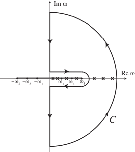
Figure 1: Integration contour in the complex plane. Dots indicate the different branch points, where we have set (without loss of generality) $\omega_{1}<\omega_{2}<\omega_{3}$. Crosses denotes the eigen-frequencies. There is a branch cut in the interval $[-\omega_{3},\omega_{3}]$ on the real axis.

One can show that the contribution to the integral of the semi-circunference vanishes. Moreover, the contribution of the segments above and below the real axis gives minus the sum over $\omega^{<}_{n}(k_{z})$. Therefore, we end up with a representation of the interaction energy as an integral on the imaginary axis

$$E_{13}=\frac{\hbar cL}{8\pi^{2}i}\int_{-\infty}^{\infty}dk_{z}\int dz\,z\frac{d}{dz}\ln[\det{\bf M}/\det({\bf M}_{\infty})].$$ (15)

From this point onwards, the calculation of the exact Casimir interaction energy between media-separated material cylinders proceeds as in the case of vacuum-separated perfectly reflecting cylinders ouroldwork . The main difference with that calculation is the presence of $R_{n}^{(1-2)}$ and $R_{n}^{(2-3)}$, both of which are equal to unity in the perfectly reflecting case. Following the same procedure as in ouroldwork , the interaction energy can be written as

$$E_{13}=\frac{\hbar cL}{4\pi^{2}}\int_{-\infty}^{\infty}dk_{z}\int_{0}^{\infty}d\xi\,\ln\det({\bf I}-{\bf A})\,\,,$$ (16)

where the matrix elements of ${\bf A}$ are

$$A_{np} = \tilde{R}^{(1-2)}_{n}\frac{I_{n}(\tilde{\lambda}_{2}a)}{K_{n}(\tilde{\lambda}_{2}a)}$$

$$\times \sum_{m}\frac{K_{m}(\tilde{\lambda}_{2}b)}{I_{m}(\tilde{\lambda}_{2}b)}\frac{1}{\tilde{R}^{(2-3)}_{n}}I_{n-m}(\tilde{\lambda}_{2}a\delta)I_{p-m}(\tilde{\lambda}_{2}a\delta).$$

The functions $\tilde{R}_{n}$ are the analytic continuation of the functions $R_{n}$ to imaginary frequencies $i\xi$:

$$\tilde{R}^{(1-2)}_{n}=R^{(1-2)}_{n}(k_{z},i\xi)=\frac{1-\frac{\tilde{\lambda}_{2}}{\tilde{\lambda}_{1}}\frac{I_{n}(\tilde{\lambda}_{1}a)I_{n}^{\prime}(\tilde{\lambda}_{2}a)}{I_{n}(\tilde{\lambda}_{2}a)I_{n}^{\prime}(\tilde{\lambda}_{1}a)}}{1-\frac{\tilde{\lambda}_{2}}{\tilde{\lambda}_{1}}\frac{I_{n}(\tilde{\lambda}_{1}a)K_{n}^{\prime}(\tilde{\lambda}_{2}a)}{I_{n}^{\prime}(\tilde{\lambda}_{1}a)K_{n}(\tilde{\lambda}_{2}a)}},$$ (18)

and

$$\tilde{R}^{(2-3)}_{n}=R^{(2-3)}_{n}(k_{z},i\xi)=\frac{1-\frac{\tilde{\lambda}_{2}}{\tilde{\lambda}_{3}}\frac{I_{n}^{\prime}(\tilde{\lambda}_{2}b)K_{n}(\tilde{\lambda}_{3}b)}{I_{n}(\tilde{\lambda}_{2}b)K_{n}^{\prime}(\tilde{\lambda}_{3}b)}}{1-\frac{\tilde{\lambda}_{2}}{\tilde{\lambda}_{3}}\frac{K_{n}(\tilde{\lambda}_{3}b)K_{n}^{\prime}(\tilde{\lambda}_{2}b)}{K_{n}^{\prime}(\tilde{\lambda}_{3}b)K_{n}(\tilde{\lambda}_{2}b)}}.$$ (19)

In order to derive this result we enclosed the system into a large cylinder, alternatively one can deal with the unbounded configuration following the approach described in Ref.nesterenko .

II.1 Attraction-repulsion crossover

In this subsection we study the condition for the crossover from attractive to repulsive interaction. For simplicity, we concentrate ourselves on the case of concentric cylinders. In the particular case of $\delta=0$ the matrix $A_{np}$ becomes diagonal, and the Casimir interaction energy reduces to

$$E_{13} = \frac{\hbar cL}{4\pi^{2}}\sum_{n}\int_{-\infty}^{\infty}dk_{z}\int_{0}^{\infty}d\xi\,$$ (20)

$$\times \ln\left[1-\frac{\tilde{R}^{(1-2)}_{n}}{\tilde{R}^{(2-3)}_{n}}\frac{I_{n}(\tilde{\lambda}_{2}a)}{K_{n}(\tilde{\lambda}_{2}a)}\frac{K_{n}(\tilde{\lambda}_{2}b)}{I_{n}(\tilde{\lambda}_{2}b)}\right].$$

We now analyze the signs of $\tilde{R}^{(1-2)}_{n}$ and $\tilde{R}^{(2-3)}_{n}$ as a function of the three permittivities $\epsilon_{i}$. For the $\tilde{R}^{(1-2)}_{n}$ coefficients, we rewrite Eq.(18) using the new variables $x\equiv\tilde{\lambda}_{2}a$ and $\tilde{\lambda}_{12}\equiv\tilde{\lambda}_{1}/\tilde{\lambda}_{2}$, obtaining

$$\tilde{R}^{(1-2)}_{n}=\frac{1-\frac{1}{\tilde{\lambda}_{12}}\frac{I_{n}(\tilde{\lambda}_{12}x)I^{\prime}_{n}(x)}{I_{n}(x)I^{\prime}_{n}(\tilde{\lambda}_{12}x)}}{1-\frac{1}{\tilde{\lambda}_{12}}\frac{I_{n}(\tilde{\lambda}_{12}x)K^{\prime}_{n}(x)}{K_{n}(x)I^{\prime}_{n}(\tilde{\lambda}_{12}x)}}.$$ (21)

Since $I_{n}(x)$, $K_{n}(x)$, and $I^{\prime}_{n}(x)$ are always positive for $x>0$, while $K^{\prime}_{n}(x)$ is always negative, the denominator in Eq.(21) is positive. Therefore, the sign of $\tilde{R}^{(1-2)}_{n}$ is determined by the numerator $N$, that can be written as

$$N=1-\frac{f(x)}{f(\lambda_{12}x)},$$ (22)

where $f(x)=x\frac{I_{n}^{\prime}(x)}{I_{n}(x)}$. It is possible to show bessels that $f(x)$ is an increasing function of $x$. Therefore $f(x)>f(\tilde{\lambda}_{12}x)$ for $\tilde{\lambda}_{12}<1$ and viceversa when $\tilde{\lambda}_{12}>1$. This implies that $\tilde{R}^{(1-2)}_{n}>0$ when $\epsilon_{1}>\epsilon_{2}$ ($\tilde{\lambda}_{12}>1$), and $\tilde{R}^{(1-2)}_{n}<0$ when $\epsilon_{1}<\epsilon_{2}$ ($\tilde{\lambda}_{12}<1$).

Using a similar argument it is possible to analyze the sign of $\tilde{R}^{(2-3)}_{n}$ as given by Eq.(19). The numerator is always positive, and then the sign of $\tilde{R}^{(2-3)}_{n}$ is governed by the denominator $D$ which reads

$$D=1-\frac{g(\tilde{\lambda}_{23}u)}{g(u)},$$ (23)

where $u=\tilde{\lambda}_{3}b$, $\tilde{\lambda}_{23}=\tilde{\lambda}_{2}/\tilde{\lambda}_{3}$, and $g(u)=-u\frac{K_{n}^{\prime}(u)}{K_{n}(u)}$. As $g(u)$ is an increasing function, it is easy to check that $\tilde{R}^{(2-3)}_{n}<0$ for $\epsilon_{2}>\epsilon_{3}$, and $\tilde{R}^{(2-3)}_{n}>0$ for $\epsilon_{2}<\epsilon_{3}$.

The sign of the Casimir interaction energy $E_{13}$ in Eq.(20) is determined by the sign of the ratio $\tilde{R}^{(1-2)}_{n}/\tilde{R}^{(2-3)}_{n}$. When this ratio is positive (negative) the energy is negative (positive). From the above considerations it follows that for $\epsilon_{1}<\epsilon_{2}<\epsilon_{3}$ (corresponding to $\tilde{R}^{(1-2)}_{n}>0$ and $\tilde{R}^{(2-3)}_{n}<0$), or for $\epsilon_{1}>\epsilon_{2}>\epsilon_{3}$ (corresponding to $\tilde{R}^{(1-2)}_{n}<0$ and $\tilde{R}^{(2-3)}_{n}>0$), the Casimir pressure is repulsive. For all other cases the Casimir pressure is attractive. Strictly speaking, the sign of the energy is not enough to determine the atractive/repulsive character of the pressure. However, we have checked using simple numerical evaluations that the integrand of Eq.(20) is always a monotonous function of $b$.

As we will see in Section IV, when the cylinders are eccentric ($\delta\neq 0$), the same conditions imply a repulsive or attractive force, with the concentric configuration being an equilibrium situation. When $\epsilon_{1}<\epsilon_{2}<\epsilon_{3}$ or when $\epsilon_{1}>\epsilon_{2}>\epsilon_{3}$ this equilibrium is stable, and it is unstable in all other situations. Just as in the case of the electromagnetic Casimir-Lifshitz interaction between media-separated planar slabs, it is only necessary that the above mentioned inequalities between the three different permittivities should hold in the relevant range of frequencies in Eq.(20). This frequency range is determined by the geometrical parameters, particularly by the minimum distance between the cylinders. In cases where the three permittivities satisfy the inequalities needed for repulsion in some frequency range, but violate them in some other frequency range, the global sign of the force results from a competition between the different contributions to the integrand in Eq.(20) (see RodriguezPRL for further details).

II.2 Perfect conductivity limit

In this subsection we study the perfect conducting limit of the expression for the interaction energy of Eq.(16). For the scalar field, “perfect conductivity” corresponds to Dirichlet boundary conditions on the interfaces. These conditions can be formally achieved for large values of the permitivities $\epsilon_{1}$ and $\epsilon_{3}$ of the two cylinders.

Using the asymptotic expansions for $I_{n}(x)$, $K_{n}(x)$, and their derivatives, it follows that in the limit $\tilde{\lambda}_{1}\rightarrow\infty$ the function $\tilde{R}^{(1-2)}_{n}$ takes the form

$$\tilde{R}^{(1-2)}_{n}\approx 1-\frac{\tilde{\lambda}_{2}}{\tilde{\lambda}_{1}}\left[\frac{I^{\prime}_{n}(\tilde{\lambda}_{2}a)}{I_{n}(\tilde{\lambda}_{2}a)}-\frac{K^{\prime}_{n}(\tilde{\lambda}_{2}a)}{K_{n}(\tilde{\lambda}_{2}a)}\right].$$ (24)

Similarly, in the limit $\tilde{\lambda}_{3}\rightarrow\infty$ the function $\tilde{R}^{(2-3)}_{m}$ takes the form

$$\tilde{R}^{(2-3)}_{n}\approx 1+\frac{\tilde{\lambda}_{2}}{\tilde{\lambda}_{3}}\left[\frac{I^{\prime}_{n}(\tilde{\lambda}_{2}b)}{I_{n}(\tilde{\lambda}_{2}b)}-\frac{K^{\prime}_{n}(\tilde{\lambda}_{2}b)}{K_{n}(\tilde{\lambda}_{2}b)}\right].$$ (25)

In this perfect-conductors limit, the matrix elements of ${\bf A}$ can be written as $A_{np}\approx A_{np}^{\rm PC}-\Delta A_{np}$, where $A_{np}^{\rm PC}$ are the matrix elements corresponding to taking the perfect conductor (PC) limit $\tilde{R}^{(1-2)}_{n}=\tilde{R}^{(2-3)}_{n}=1$ (see ouroldwork ), and

$$\Delta A_{np}=\frac{\tilde{\lambda}_{2}}{{\tilde{\lambda}}_{1}}\left[\frac{I^{\prime}_{n}(\tilde{\lambda}_{2}a)}{I_{n}(\tilde{\lambda}_{2}a)}-\frac{K^{\prime}_{n}(\tilde{\lambda}_{2}a)}{K_{n}(\tilde{\lambda}_{2}a)}\right]$$

$$\times\frac{I_{n}(\tilde{\lambda}_{2}a)}{K_{n}(\tilde{\lambda}_{2}a)}\sum_{m}\frac{K_{m}(\tilde{\lambda}_{2}b)}{I_{m}(\tilde{\lambda}_{2}b)}I_{n-m}(\tilde{\lambda}_{2}a\delta)I_{p-m}(\tilde{\lambda}_{2}a\delta)$$

$$+\frac{\tilde{\lambda}_{2}}{{\tilde{\lambda}}_{3}}\frac{I_{n}(\tilde{\lambda}_{2}a)}{K_{n}(\tilde{\lambda}_{2}a)}\sum_{m}\left[\frac{I^{\prime}_{m}(\tilde{\lambda}_{2}b)}{I_{m}(\tilde{\lambda}_{2}b)}-\frac{K^{\prime}_{m}(\tilde{\lambda}_{2}b)}{K_{m}(\tilde{\lambda}_{2}b)}\right]$$

$$\times\frac{K_{m}(\tilde{\lambda}_{2}b)}{I_{m}(\tilde{\lambda}_{2}b)}I_{n-m}(\tilde{\lambda}_{2}a\delta)I_{p-m}(\tilde{\lambda}_{2}a\delta).$$ (26)

The Casimir interaction energy is therefore $E_{13}\approx E_{13}^{\rm PC}+\Delta E_{13}$, where

$$\Delta E_{13} = -\frac{\hbar cL}{4\pi^{2}}\int_{-\infty}^{\infty}dk_{z}\int_{0}^{\infty}d\xi\;{\rm Tr}\;\frac{\Delta{\bf A}}{1-{\bf A}^{\rm PC}}.$$ (27)

In this limit, and assuming that the $\epsilon_{i}$ are constants (i.e., no dispersion), it is possible to obtain the explicit dependence of the interaction energy $\Delta E_{13}$ on the three permittivities. The key point is to note that

$$\Delta E_{13} = \frac{\hbar cL}{4\pi^{2}}\int_{-\infty}^{\infty}dk_{z}\int_{0}^{\infty}d\xi\left(\frac{1}{\tilde{\lambda}_{1}}f_{1}(\tilde{\lambda}_{2},a,b,\delta)\right.$$ (28)

$$+ \left.\frac{1}{\tilde{\lambda}_{3}}f_{2}(\tilde{\lambda}_{2},a,b,\delta)\right)\,\,,$$

for some functions $f_{i}$. We change variables in the integral above introducing polar coordinates $(\eta,\varphi)$ in the plane $(\sqrt{\epsilon_{2}}\xi/c,k_{z})$, so that $\tilde{\lambda}_{2}=\eta$ and $\tilde{\lambda}_{i}=\eta\sqrt{(\epsilon_{i}/\epsilon_{2}-1)\cos^{2}\varphi+1}$ for $i=1,3$. The integral in $\varphi$ can be computed explicitly and gives

$$\int_{0}^{2\pi}\frac{d\varphi}{\sqrt{(\epsilon_{i}/\epsilon_{2}-1)\cos^{2}\varphi+1}}\approx\sqrt{\frac{\epsilon_{2}}{\epsilon_{i}}}\ln\left(\frac{\epsilon_{i}}{\epsilon_{2}}\right)$$ (29)

for $\epsilon_{1},\epsilon_{3}\rightarrow\infty$. Inserting this result in Eq.(28) we obtain

$$\frac{\Delta E_{13}}{L}\approx\frac{\ln(\epsilon_{1}/\epsilon_{2})}{\sqrt{\epsilon_{1}}}G_{1}(a,b,\delta)+\frac{\ln(\epsilon_{3}/\epsilon_{2})}{\sqrt{\epsilon_{3}}}G_{2}(a,b,\delta)\,,$$ (30)

where the functions $G_{i}$ involve integrals in the radial coordinate $\eta$.

In previous works Milton , the Casimir energy was evaluated using dilute-limit expansions. Eq.(30) gives the dependence with the permittivities in the opposite limit. The result shows that the convergence to the case of perfect conductivity is rather slow.

III Cylinder-plane geometry

In the case of perfect conductors, we have shown in ouroldwork that the cylinder-plane configuration is contained as a particular case of the exact formula for eccentric cylinders. In this Section we obtain the matrix elements for the cylinder-plane configuration from the media-separated cylinders Eqs. (16) and (II). As in ouroldwork , let us consider a cylinder of radius $a$ above an infinite plane. The permittivities are $\epsilon_{1}$ inside the cylinder, $\epsilon_{2}$ between the cylinder and the plane, and $\epsilon_{3}$ in the region below the plane. Let us denote by $H$ the distance between the center of the cylinder and the plane. The expression for the interaction energy in the media-separated cylinder-plane geometry can be obtained from the eccentric cylinders formula Eq. (16) taking the limit $b/a$, $\delta\rightarrow\infty$, keeping $H/a=b/a-\delta$ fixed. Using the asymptotic limit of the Bessel functions, it is possible to show that the coefficient ${\tilde{R}}_{n}^{(2-3)}\rightarrow\frac{{\tilde{\lambda}}_{3}+{\tilde{\lambda}}_{2}}{{\tilde{\lambda}}_{3}-{\tilde{\lambda}}_{2}}$, and therefore it can be taken outside the sum in Eq. (II). After this, and making use of the uniform expansion and the addition theorem of Bessel functions, it can be also shown that ouroldwork

$$\sum_{m}\frac{K_{m}(y+l)}{I_{m}(y+l)}I_{m-n}(y)I_{m-p}(y)$$ (31)

$$\approx \sum_{m}K_{m}(y+l)I_{m-p-n}(y-l)=K_{n+p}(2l),$$

in the limit $y\rightarrow\infty$. Finally, the expression for the matrix elements in the cylinder-plane geometry is given by

$$A_{np}^{\rm cp}={\tilde{R}}_{n}^{(1-2)}\frac{{\tilde{\lambda}}_{3}-{\tilde{\lambda}}_{2}}{{\tilde{\lambda}}_{3}+{\tilde{\lambda}}_{2}}\frac{I_{n}({\tilde{\lambda}}_{2}a)}{K_{n}({\tilde{\lambda}}_{2}a)}K_{n+p}(2{\tilde{\lambda}}_{2}H).$$ (32)

This generalizes the result of cil-plane for vacuum-separated, perfectly conducting cylinder-plane to the three-media cylinder-plane geometry.

The sign of the Casimir interaction energy for the cylinder-plane geometry is ruled by the signs of ${\tilde{R}}_{n}^{(1-2)}$ and $({\tilde{\lambda}}_{3}-{\tilde{\lambda}}_{2})/({\tilde{\lambda}}_{3}+{\tilde{\lambda}}_{2})$. The attractive-repulsive character of the force depends on the relative values of $\epsilon_{1}$, $\epsilon_{2}$ and $\epsilon_{3}$, in the same way as for the eccentric cylinders.

The dependence of the Casimir energy on the permittivities in the perfect conductivity limit can also be derived from Eq.(32). The procedure is similar to the one used to obtain Eq.(30), so we only quote the final result

$$\frac{\Delta E_{13}^{\rm cp}}{L}\approx\frac{\ln(\epsilon_{1}/\epsilon_{2})}{\sqrt{\epsilon_{1}}}G^{\rm cp}_{1}(a,d)+\frac{\ln(\epsilon_{3}/\epsilon_{2})}{\sqrt{\epsilon_{3}}}G^{\rm cp}_{2}(a,d)\,,$$ (33)

for some functions $G^{\rm cp}_{i}$. In the next Section we will provide numerical evaluations that confirm this behavior.

IV Numerical evaluations

In this Section, we show numerical results for the Casimir interaction energy between eccentric media separated cylinders and a cylinder in front of an infinite plane. For simplicity, we consider the dispersion-less case in which $\epsilon_{i}$ are constants.

The value of the Casimir interaction energy is obtained by the numerical evaluation of Eq.(16), through the use of the different definitions of the matrix elements $A_{np}$ depending upon the geometry considered (Eqs.(II) and (32)). We numerically compute the Casimir interaction energy using a FORTRAN program which defines the matrix elements of $\mathbf{A}$, computes the corresponding eigenvalues. and finally performs the frequency and wavevector integrations. The parameters used by the program are the dimension of the ${\bf M}$ matrix, the number of addends corresponding to each element of the ${\bf M}$ matrix, the integration limits ${k_{z}}_{\rm max}$ and $\xi_{\rm max}$, and the desired precision. In the following, we show the numerical results obtained.

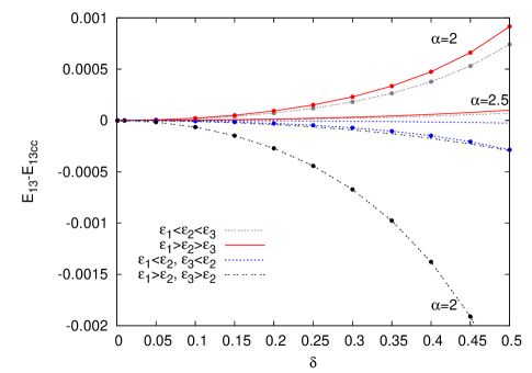
Figure 2: (Color online). Exact Casimir interaction energy difference between the eccentric and concentric configurations as a function of $\delta$ for different values of $\alpha=b/a$. Curves with circles correspond to $\alpha=2.0$, while those without circles correspond to $\alpha=2.5$. In all cases $\epsilon_{1}=2$, $\epsilon_{2}=5$ and $\epsilon_{3}=50$, ordered as indicated in the legend. Energy is plotted in units of $\hbar cL$.

Fig. 2 shows the interaction energy difference between the eccentric and concentric configurations as a function of the dimensionless eccentricity $\delta$. There are two sets of parameters used, namely for $\alpha=b/a=2.0$ and $\alpha=2.5$. We have used $\epsilon_{1}=2$, $\epsilon_{2}=5$ and $\epsilon_{3}=50$ in all cases, varying the relative order among them: $\epsilon_{1}<\epsilon_{2}<\epsilon_{3}$ and $\epsilon_{1}>\epsilon_{2}>\epsilon_{3}$ for the positive curves, while $\epsilon_{1}<\epsilon_{2}$, $\epsilon_{3}<\epsilon_{2}$ and $\epsilon_{1}>\epsilon_{2}$, $\epsilon_{3}>\epsilon_{2}$ for the negative ones. The plot clearly shows the change of the sign of the energy depending on the relative order among the dielectric constants, and also the unstable/stable equilibrium position at the concentric configuration.

In order to analyze the dependence of the sign of the force in the cylinder-plane geometry on the relation between $\epsilon_{1}$, $\epsilon_{2}$, and $\epsilon_{3}$ we show in Fig.3 the exact Casimir interaction energy a function of the minimum distance between the cylinder and the plane $d=H-a$. Again, we plot different orderings of the dielectric constants. It is easy to note that for a decreasing or increasing ordering of the dielectric constants, we get a repulsive force, while in any other case the force is attractive.

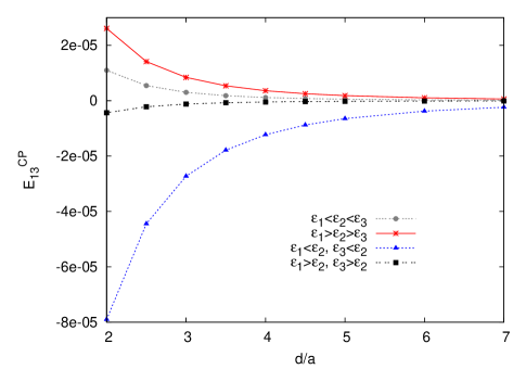
Figure 3: (Color online). Exact Casimir interaction energy for the cylinder-plane configuration as a function of the minimum distance between the cylinder and the plane. In the upper curves, we show the energy for the cases in which $\epsilon_{1}<\epsilon_{2}<\epsilon_{3}$ or $\epsilon_{1}>\epsilon_{2}>\epsilon_{3}$, and the force is repulsive. The opposite case is shown in the lower part of the plot. In these cases $\epsilon_{1}>\epsilon_{2}$, $\epsilon_{3}>\epsilon_{2}$ or $\epsilon_{1}<\epsilon_{2}$, $\epsilon_{3}<\epsilon_{2}$, and therefore the force is attractive. Energy is plotted in units of $\hbar cL$.

Finally, in Fig. 4 we numerically check Eq.(33) with $\epsilon_{3}\to\infty$. In this plot we show the difference between the interaction energy for the scalar dielectric example and the perfectly conducting case, as a function of $\log\epsilon_{1}/\sqrt{\epsilon_{1}}$ (different values of the distance to the plane are considered).

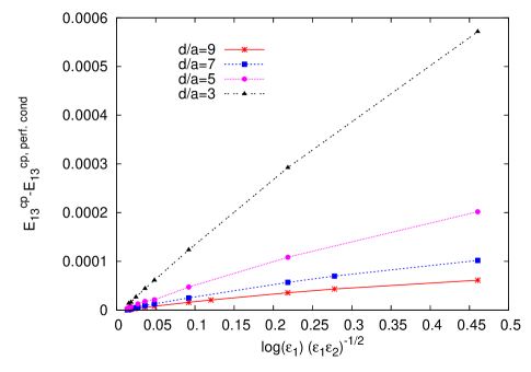
Figure 4: (Color online). Exact Casimir interaction energy difference between the dielectric cylinder-plane and the perfect conductors configurations. As can be seen in Eq.(33), the convergence to the perfect conductors case is ruled by a $\ln\epsilon_{1}/\sqrt{\epsilon_{1}}$ coefficient, making it slower than the naively expected from a simple $1/\epsilon_{1}$ decay. In this plot we have set $\epsilon_{2}=1$. Energy is plotted in units of $\hbar cL$.

V Conclusions

We have derived the exact expression for the scalar Casimir interaction energy between media-separated eccentric cylinders, and obtained the cylinder-plane result as a particular case. In analogy with the well-known electromagnetic Casimir-Lifshitz interaction energy between fluid-separated planes, our results show that the force in the two non-planar geometries studies can be repulsive or attractive depending on the relative strength of the permittivities of the three intervening media over a broad range of frequencies. We have presented both analytical and numerical calculations to prove that this is indeed the case regardless the value of the radii of the cylinders and of the eccentricity.

We have considered the case of a quantum scalar field. The analogous calculation for the full electromagnetic field is much more involved. The reason is that, unlike the case of perfect reflectors, TE and TM modes do not decouple for finite values of the permittivities, and this fact introduces algebraic complications in the derivation of the exact formula presented in Section II. We expect to analyze this issue in a future publication.

VI Acknowledgments

We thank J. Etcheverry and F. Intravaia for useful discussions. The work of DARD was funded by DARPA/MTO’s Casimir Effect Enhancement program under DOE/NNSA Contract DE-AC52-06NA25396. FCL and FDM were supported by UBA, CONICET, and ANPCyT, Argentina. PIV acknowledges support of UNESCO LOREAL For Women in Science Programme.

References

- (1) H. B. G. Casimir, Proc. K. Ned. Akad. Wet. 51, 793 (1948).
- (2) E. M. Lifshitz, Sov. Phys. JETP 2, 73 (1956).
- (3) A. A. Feiler, L. Bergstrom, and M. W. Rultand, Langmuir 24, 2274 (2008); J. N. Munday, F. Capasso, and V. A. Parsegian, Nature 457, 170 (2009); and references therein.
- (4) B. V. Derjaguin and I. I. Abrikosova, Sov. Phys. JETP 3, 819 (1957); B. V. Derjaguin, Sci. Am. 203, 47 (1960).
- (5) V. A. Parsegian, Van der Waals Forces (Cambridge University Press, Cambridge, 2006).
- (6) K. A. Milton, P. Parashar, and J. Wegner, Phys. Rev. Lett. 101, 160402 (2008); K. A. Milton, P. Parashar, and J. Wagner, arXiv:0811.0128.
- (7) R. Golestanian, Phys. Rev. A 80, 012519 (2009).
- (8) T. Emig, N. Graham, R. L. Jaffe, and M. Kardar, Phys. Rev. Lett. 99, 170403 (2007); S. J. Rahi, T. Emig, N. Graham, R. L. Jaffe, and M. Kardar, Phys. Rev. D 80, 085021 (2009).
- (9) P. A. Maia Neto, A. Lambrecht, and S. Reynaud, Phys. Rev. A 78, 012115 (2008).
- (10) O. Kenneth and I. Klich, Phys. Rev. B 78, 014103 (2008).
- (11) R. Messina, D. A. R. Dalvit, P. A. Maia Neto, A. Lambrecht, and S. Reynaud, Phys. Rev. A 80, 022119 (2009).
- (12) D. A. R. Dalvit, F. C. Lombardo, F. D. Mazzitelli, and R. Onofrio, Phys. Rev. A 74, 020101(R) (2006); F. D. Mazzitelli, D. A. R. Dalvit, and F. C. Lombardo, New Journal of Physics 8, 240 (2006).
- (13) F.C. Lombardo, F.D. Mazzitelli, and P.I. Villar, Phys. Rev. D 78, 085009 (2008).
- (14) A. W. Rodriguez, A. P. McCauley, J. D. Joannopoulos, and S. G. Johnson, Phys. Rev. A 80, 012115 (2009); M. T. H. Reid, A. W. Rodriguez, J. White, and S. G. Johnson, Phys. Rev. Lett. 103, 040401 (2009).
- (15) H. Gies, K. Langfeld, and L. Moyaerts, J. High Energy Phys. 06, 018 (2003).
- (16) F.C. Lombardo, F.D. Mazzitelli, M. Vázquez, and P.I. Villar, Phys. Rev. D 80, 065018 (2009); F.C. Lombardo, F.D. Mazzitelli, and P.I. Villar, Proceedings of QFEXT09; eds. Kimball A. Milton and Michael Bordag, World Scientific, Singapore (2010); arXiv:1003.2011
- (17) A. W. Rodriguez, J. N. Munday, J. D. Joannopoulos, F. Capasso, D. A. R. Dalvit, and S. G. Johnson, Phys. Rev. Lett. 101, 190404 (2008).
- (18) S.J. Rahi and S. Zaheer, Phys. Rev. Lett. 104, 070405 (2010).
- (19) F. S. S. Rosa, D. A. R. Dalvit, and P. W. Milonni, Phys. Rev. A 81, 033812 (2010); arXiv:0912.0279.
- (20) F. Intravaia and C. Henkel, J. Phys. A: Math. Gen. 41, 164018 (2008).
- (21) V.V. Nesterenko, J.Phys. A: Math. Theor. 41, 164005 (2008).
- (22) V. V. Nesterenko and I. G. Pirozhenko, arXiv:1003.0886 [hep-th].
- (23) See Eq. (3.7) in C.M. Joshi and S.K. Bissu, J. Austral. Math. Soc. (Series A) 50, 333 (1991).
- (24) T. Emig, R.L. Jaffe, M. Kardar, and A. Scardicchio, Phys. Rev. Lett. 96, 080403 (2006); M. Bordag, Phys. Rev. D 73, 125018 (2006).