Algebraic Comparison of Partial Lists in Bioinformatics

Abstract

The outcome of a functional genomics pipeline is usually a partial list of genomic features, ranked by their relevance in modelling biological phenotype in terms of a classification or regression model. Due to resampling protocols or just within a meta-analysis comparison, instead of one list it is often the case that sets of alternative feature lists (possibly of different lengths) are obtained. Here we introduce a method, based on the algebraic theory of symmetric groups, for studying the variability between lists (“list stability”) in the case of lists of unequal length. We provide algorithms evaluating stability for lists embedded in the full feature set or just limited to the features occurring in the partial lists. The method is demonstrated first on synthetic data in a gene filtering task and then for finding gene profiles on a recent prostate cancer dataset.

1 INTRODUCTION

Defining indicators for assessing ranked lists variability has become a key research issue in functional genomics [1, 2, 3, 4, 5].

In [6], a method is introduced to detect stability (homogeneity) of a set of ranked lists of biomarkers emerging as output of feature selection algorithm during a molecular profiling task. The stability indicator relies on the application of metric methods for ordered data viewed as elements of a suitable permutation group: foundations of such theory can be found in [7, 8] and it is based on the concept of distance between two lists; in particular, the employed metric is the Canberra distance as discussed in [9]. The mathematical details of the stability procedure are described in [10, 11]: given a set of ordered lists, the basic mechanism is to evaluate the degree of self-homogeneity of a set of ordered lists through the computation of all the mutual distances between the elements of the original set. Moreover, by using the location parameter, the Canberra distance can also be computed between upper partial lists of the original complete lists, the so called top-$k$ lists [12], formed by their $k$ best ranked elements. The method proposed in [6] has a main drawback limiting its application in many practical situations: the studied lists are required to have the same length. As complete lists, they all share the same elements, with only their ordering being different and, when considering partial top-$k$ lists, the same $k$ must be chosen for all sublists.

This is usually not the case when investigating the outcomes of profiling experiments where the employed feature ranking method does not produce a rank for every involved feature, but it just scores the best performing ones, thus leading to the construction of lists with different lengths. Some work towards partial lists comparison has recently appeared in literature, both for general contexts [13] and more focussed on the gene ranking case [14, 15, 16], but they all consist of set-theoretical measures.

In the present work we propose an extension of the method introduced in [6] to mend this flaw by allowing computing (Canberra) distance for two lists of different length, defined within the framework of the metric methods for permutation groups. The novel approach is based on the use of quotients of permutation groups. The key formula can be split into two main components: one taking care of the elements occurring in the selected lists, and the second one considering the remaining elements of the complete set of features the experiment started from. In particular, this second component is independent from the positions of the selected elements in the lists: neglecting this part, a different stability measure (called the core component of the complete formula) is obtained. An applications of the described methods can be found in [17].

After having detailed the central algorithm in Section 2, applications to synthetic and genomics datasets and different machine learning tasks are discussed in Section 3. The described algorithm is publicly available within the Python package mlpy (https://mlpy.fbk.eu) for statistical machine learning.

2 MATERIALS AND METHODS

2.1 Introduction

The procedure described in [6] is made of two separate parts, the former concerning the computation of all the mutual distances between the (complete or partial) lists, and the latter the construction of the matrix starting from those distances and of the indicator coming from the defined matrix. This second phase is independent from the length of the considered lists: the extension shown hereafter only affects the previous step, i.e. the distance definition. The algorithm relies on application of metric methods for ordered data viewed as elements of a suitable permutation group: foundations of such theory can be found in [18, 19, 7, 8] and it is based on the concept of distance between two lists; in particular, the employed metric is the Canberra distance [9]. The mathematical details of the procedure are shown in [10, 11]. The described algorithm defines a measure to evaluate the degree of self-homogeneity of a set of ordered lists through the computation of all the mutual distances between the elements of the original set. Moreover, the distance can also be computed between upper partial lists of the original complete lists, the so called top-$k$ lists [12], formed by their $k$ best ranked elements. The indicator introduced in [6] has a main drawback limiting its application in many practical situations: the studied lists are required to have the same length. In fact, as complete lists they must share the same elements, with only their ordering being different and, when considering partial top-$k$ lists, the same $k$ must be chosen for all sublists. This is usually not the case when investigating the outcomes of profiling experiments where the employed feature ranking method does not produce a rank for every involved feature, but it just scores the best performing ones, thus leading to the construction of lists with different length. Some work towards this task has recently appeared in literature, both for general contexts [13] and more focussed on the gene ranking case [14, 15, 16], but they all consist of set-theoretical measure. In the present work we propose an extension of the method introduced in [6] to mend this flaw by allowing computing (Canberra) distance for two lists of different length, still defined within the framework of the metric methods for permutation groups.

2.2 Notations

Let $\mathcal{F}=\{F_{j}\}_{j=1,\ldots,p}$ be a set of $p$ features, and let $L$ be a ranked list consisting of $l$ elements extracted (without replacement) from $\mathcal{F}$. If $L=\left(F_{L_{1}},F_{L_{2}},\ldots,F_{L_{l}}\right)$, let $\tau(j)$ be the rank of $F_{j}$ in L (with $\tau(F_{z})=0$ if $F_{z}\not\in L$) and define $\tau=\left(\tau(j)\right)_{j=1,\ldots,p}$ the dual list of $L$. Consider the set ${S}_{L}$ of all elements of the symmetric group $S_{\mathcal{F}}$ on $\mathcal{F}$ whose top-$l$ sublist is $L$: ${S}_{L}$ has $(p-l)!$ elements and it is isomorphic to (a coset of) $S_{p-l}$. Finally, let ${S}_{\tau}$ be the set of all the dual lists of the elements in ${S}_{L}$: if $\alpha\in{S}_{\tau}$, then $\alpha(i)=\tau(i)$ for all indexes $i\in L$. Thus $S_{\tau}$ consists of the $(p-|L|)!$ (dual) permutations of $S_{p}$ coinciding with $\tau$ on the elements belonging to $L$. Furthermore, note that $\tau(L)=\{1,\ldots,|L|\}$.

2.3 Shorthands

If $H_{s}$ is used to denote the $s$-th armonic number defined as $\displaystyle{H_{s}=\sum_{j=1}^{s}\frac{1}{j}}$, then we can define some useful shorthands:

$$\begin{split}&\Delta(a,b,c)=\sum_{a\leq i\leq b}\frac{|c-i|}{c+i}\\ &=\begin{cases}b-a+1-2c(H_{b+c}-H_{a+c-1})\\ \mbox{\hskip 120.00018pt}\textrm{if $c<a$}\\ 2c(H_{2c}-H_{a+c-1}-H_{b+c}-1)+b+a-1\\ \mbox{\hskip 120.00018pt}\textrm{if $a\leq c\leq b$}\\ 2c(H_{b+c}-H_{a+c-1})-b+a-1\\ \mbox{\hskip 120.00018pt}\textrm{if $c>b$}\ ,\end{cases}\end{split}$$

and

$$\varepsilon_{k}(s) {}={}\sum_{j=1}^{s}jH_{j+k}$$

$${}={}\frac{(s-k)(s+k+1)}{2}H_{s+k+1}+\frac{k(k+1)}{2}H_{k+1}$$

$$+\frac{s(2k-s-1)}{4}$$

$$\xi(s) {}={}\sum_{j=1}^{s}(2j)H_{2j}$$

$${}={}\left(s+\frac{1}{2}\right)^{2}H_{2s+1}-\frac{1}{8}H_{s}-\left(\frac{2s^{2}+s+1}{4}\right)\ .$$

Finally,

$$\Theta(\alpha,\beta,\gamma)=\sum_{\alpha\leq u\leq\gamma}\sum_{\beta\leq v\leq\gamma}\frac{|u-v|}{u+v}=\sum_{\alpha\leq u\leq\gamma}\Delta(\beta,\gamma,u)\ ,$$

with $\Theta(\alpha,\beta,\gamma)=\Theta(\beta,\alpha,\gamma)$. Details on harmonic number can be found in [20], while some new techniques for dealing with sums and products of harmonic numbers are shown in [21, 22, 23, 24, 25, 26, 27, 28, 29].

2.4 Canberra distance on permutation groups

Given two real-valued vectors $\mathbf{x},\mathbf{y}\in\mathbb{R}^{n}$, their Canberra distance [9] is defined as

$$\operatorname{Ca}(\mathbf{x},\mathbf{y})=\sum_{i=1}^{n}\frac{|\mathbf{x}_{i}-\mathbf{y}_{i}|}{|\mathbf{x}_{i}|+|\mathbf{y}_{i}|}\ .$$

This metric can be naturally extended to a distance on permutation groups: for $\tau,\sigma\in S_{p}$, we have

$$\operatorname{Ca}(\tau,\sigma)=\sum_{i=1}^{p}\frac{|\tau(i)-\sigma(i)|}{\tau(i)+\sigma(i)}\ .$$

The expected (average) value of the Canberra metric on the whole group $S_{p}$ can be computed as follows:

$$E\{\operatorname{Ca}(S_{p})\} =\frac{1}{|S_{p}|^{2}}\sum_{\sigma,\tau\in S_{p}}\operatorname{Ca}(\sigma,\tau)$$

$$=\frac{1}{|S_{p}|}\sum_{\sigma\in S_{p}}\operatorname{Ca}(\sigma,\mathrm{Id}_{S_{p}})$$

$$=\frac{1}{p!}\sum_{\sigma\in S_{p}}\sum_{i=1}^{p}\frac{|\sigma(i)-i|}{\sigma(i)+i}$$ (1)

$$=\left(2n+2+\frac{1}{2n}\right)H_{2n}$$

$$\quad{-}\left(2n+2+\frac{1}{4n}\right)H_{n}-\left(n+\frac{3}{2}\right)\ .$$

2.5 Canberra Distance on Partial Lists

If $L_{1}$ and $L_{2}$ are two (partial) lists of length respectively $l_{1}\leq l_{2}$ whose elements belong to $\mathcal{F}$, and $d$ is a distance on permutation groups, define the distance between $L_{1}$ and $L_{2}$ as

$$d(L_{1},L_{2}) =f\left(\left\{d(\alpha,\beta)\colon\alpha\in{S}_{\tau_{1}},\beta\in{S}_{\tau_{2}}\right\}\right)$$

$$=f(d({S}_{\tau_{1}},{S}_{\tau_{2}}))\ ,$$

for $f$ a function of the $(p-l_{1})!(p-l_{2})!$ distances $d(\alpha,\beta)$ such that on a singleton $t$, $f(\{t\})=t$. Note that if $L_{1}$ and $L_{2}$ are complete lists, the above definition coincides on complete lists with the usual definition of distance between complete lists given in [6]. Moreover, being $d$ a distance, the smaller the value the more similar the compared lists. A natural choice for the function $f$, motivated also from the fact that the many distances for permutation groups (and we proved this is the case for the Canberra distance in [11, 10]) are asymptotically normal [30], is the mean function, so that

$$d(L_{1},L_{2})=\frac{1}{|{S}_{\tau_{1}}|\cdot|{S}_{\tau_{2}}|}\sum_{\alpha\in{S}_{\tau_{1}}}\sum_{\beta\in{S}_{\tau_{2}}}d(\alpha,\beta)\ .$$ (2)

We note that this definition differs from the one first introduced in [6] because the relation between the size of actually used features and the size the original feature set is taken into account here. This is relevant while performing genomic profiling experiments. Consider the decomposition of the set $\mathcal{F}$ into the three disjoint sets (ignoring the features’ rank) $F_{12}=L_{1}{}\cap{}L_{2}\$, $F_{\overline{12}}=\mathcal{F}\setminus\left(L_{1}{}\cup{}L_{2}\right)$ and $F_{1/2}=\left(L_{1}{}\cup{}L_{2}\right)\setminus{}\left(L_{1}{}\cap{}L_{2}\right)$. Then, if $d=\operatorname{Ca}$ is the Canberra distance and $\displaystyle{\Lambda=\frac{1}{(p-l_{1})!(p-l_{2})!}}$, the Eq. (2) can be split as follows into three terms:

$$\operatorname{Ca}(L_{1},L_{2})=\frac{1}{|S_{\tau_{1}}|}\frac{1}{|S_{\tau_{2}}|}\sum_{\alpha\in{S}_{\tau_{1}}}\sum_{\beta\in{S}_{\tau_{2}}}\operatorname{Ca}(\alpha,\beta)$$

$$=\Lambda\sum_{\begin{smallmatrix}\alpha\in S_{p},\beta\in S_{p}\\ \alpha(i)=\tau_{1}(i)\textrm{ if $i\in L_{1}$ }\\ \beta(i)=\tau_{2}(i)\textrm{ if $i\in L_{2}$ }\end{smallmatrix}}\sum_{i=1}^{p}\frac{|\alpha(i)-\beta(i)|}{\alpha(i)+\beta(i)}\ ,$$

$$=\Lambda\sum_{(\alpha,\beta)\in S_{\tau_{1}}\times S_{\tau_{2}}}\sum_{F_{i}\in\mathcal{F}}\frac{|\alpha(i)-\beta(i)|}{\alpha(i)+\beta(i)}$$

$$=\Lambda\sum_{F_{i}\in\mathcal{F}}\sum_{(\alpha,\beta)\in S_{\tau_{1}}\times S_{\tau_{2}}}\frac{|\alpha(i)-\beta(i)|}{\alpha(i)+\beta(i)}$$

$$=\Lambda\sum_{F_{i}\in F_{12}\cup F_{1/2}\cup F_{\overline{12}}}\sum_{(\alpha,\beta)\in S_{\tau_{1}}\times S_{\tau_{2}}}\frac{|\alpha(i)-\beta(i)|}{\alpha(i)+\beta(i)}$$

$$=\Lambda\left(\sum_{F_{i}\in F_{12}}\sum_{(\alpha,\beta)\in S_{\tau_{1}}\times S_{\tau_{2}}}\frac{|\alpha(i)-\beta(i)|}{\alpha(i)+\beta(i)}\right.$$ (T1)

$$\qquad{+}\sum_{F_{i}\in F_{1/2}}\sum_{(\alpha,\beta)\in S_{\tau_{1}}\times S_{\tau_{2}}}\frac{|\alpha(i)-\beta(i)|}{\alpha(i)+\beta(i)}$$

$$\qquad{+}\left.\sum_{F_{i}\in F_{\overline{12}}}\sum_{(\alpha,\beta)\in S_{\tau_{1}}\times S_{\tau_{2}}}\frac{|\alpha(i)-\beta(i)|}{\alpha(i)+\beta(i)}\right)\ .$$

Expanding the three terms T1, T2, T3 a closed form for the distance can be reached:

Definition 1. Complete Canberra Distance. The Complete Canberra Distance (between partial lists) is defined as

$$\operatorname{Ca}(L_{1},L_{2}) =\sum_{i\in L_{1}\cap L_{2}}\left(\frac{|\tau_{1}(i)-\tau_{2}(i)|}{\tau_{1}(i)+\tau_{2}(i)}\right.$$

$$\quad\qquad\left.{-}\>\frac{\Delta(l_{2}+1,p,\tau_{1}(i))}{p-l_{2}}\right.$$ (3)

$$\quad\qquad\left.{-}\>\frac{\Delta(l_{1}+1,p,\tau_{2}(i))}{p-l_{1}}\right)$$

$$\qquad{+}\>\frac{1}{p-l_{2}}\left(l_{1}(p-l_{2})-2\varepsilon_{p}(l_{1})+2\varepsilon_{l_{2}}(l_{1})\right)$$

$$\qquad{+}\>\frac{1}{p-l_{1}}\left(l_{1}(p-l_{1})+4\varepsilon_{l_{1}}(l_{1})+2\xi(l_{2})\right.$$

$$\qquad\left.{-}\>2\xi(l_{1})-2\varepsilon_{l_{1}}(l_{2})-2\varepsilon_{p}(l_{2})\right.$$

$$\qquad\left.{+}\>(p+l_{1})(l_{2}-l_{1})+l_{1}(l_{1}+1)\right.$$

$$\qquad\left.{-}\>l_{2}(l_{2}+1)\right)$$

$$\qquad{+}\>A\cdot\left(2\xi(p)-2\xi(l_{2})-2\varepsilon_{l_{1}}(p)+2\varepsilon_{l_{1}}(l_{2})\right.$$

$$\qquad\left.{-}\>2\varepsilon_{p}(p)+2\varepsilon_{p}(l_{2})+(p+l_{1})(p-l_{2})\right.$$

$$\qquad\left.{+}\>l_{2}(l_{2}+1)-p(p+1)\right)\ ,$$

where $\displaystyle{A=\frac{|\mathcal{F}\setminus(L_{1}\cup L_{2})|}{(p-l_{1})(p-l_{2})}}$ . The sum generating the term T3 in Eq. (2.5) runs over the subset $F_{\overline{12}}$ collecting all elements of the original feature set which do not occur neither in the first list nor in the second. Thus this part of the formula is independent from the positions of the elements occurring in the partial lists $L_{1}$, $L_{2}$. Neglecting this term, we obtain another measure of list difference:

Definition 2. Core Canberra Distance. The Core Canberra is defined as the components T1, T2 of the Complete Canberra Distance depending on the positions of the elements in the considered partial lists. This corresponds to setting $A=0$ in Eq. (2.5) of Def. 2.5.

Throughout the paper, the values of both instances of the Canberra Distance are normalized by dividing them by the expected value $E\{\operatorname{Ca}(S_{p})\}$ on the whole permutation group $S_{p}$ reported in Eq. (2.4). This would result in two random (complete) lists having a Complete Canberra Distance very close to one; note that, since the expected value is not the highest one, distance values greater than one can occur. When the number of features in $\mathcal{F}$ not occurring in $L_{1}$, $L_{2}$ becomes larger, the non-core component gets numerically highly preeminent: in fact, in the term T3 all the possible $(p-l1)!(p-l2)!$ lists in $S_{p}$ having $L_{1}$ and $L_{2}$ respectively as top lists are considered; as an example, for $p=10000$ and $L_{1}$, $L_{2}$ two partial lists with $100$ elements, this corresponds in evaluating the distance among $9900!^{2}\simeq 2.2\cdot 10^{70519}$ lists of elements not occurring in $L_{1}$, $L_{2}$. When the number of lists of unselected elements grows larger, the average distance among them would get closer to the expected value of the Canberra distance on $S_{p}$ because of the Hoeffding’s Theorem.

This is quite often the case for biological ranked lists: for instance, selecting a panel of biomarkers from a set of probes usually means choosing less than hundred of features out of an original set of several thousands. Thus, considering the Core component instead of the Complete Distance can be helpful in term of dimensionality reduction of the considered problem.

As an example, in Tab. 1 we show the values of the normalized distances of two partial lists of length $10$ extracted from an original set $\mathcal{F}$ with $p=10^{c}$ features ($c=2,3,4,5$), in the three cases of identical partial lists, randomly permuted partial lists (which yields average distance) and maximally distant partial lists (see [10, 11] for the identification of the permutation maximizing the Canberra distance between lists).

Lists	Dist.	$c=2$	$c=3$	$c=4$	$c=5$
Identical	Comp.	0.692830	0.960499	0.995858	0.999583
Random	Core	0.078038	0.006368	0.000950	0.000109
Random	Comp.	0.770868	0.966867	0.996809	0.999692
Max.Dist.	Core	0.128448	0.012665	0.001265	0.000126
Max.Dist.	Comp.	0.821278	0.973164	0.997123	0.999709

Table 1: Core and Complete normalized Canberra distance for two partial lists of 10 features extracted from a set of $|\mathcal{F}|={10}^{c}$ features. The partial lists are either identical, randomly permuted (average distance) or maximally distant. The Core Distance for Identical partial lists is zero.

A further observation can be derived from Fig. 1, where the ratio between Core and Canberra distances are plotted versus the ratio between the length of partial lists and the size of the full feature set for about 7000 instances of couples of partial lists of the same length randomly permuted. When the number of elements of the partial lists is a small portion of the total feature, the Complete and the Core distance are almost linearly dependent, while when such ratio approaches one the ratio between the two measures follows a different function.

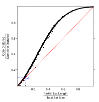
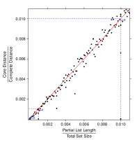
a b

Figure 1: (a) Ratio between Core and Complete distances versus ratio between the length of partial lists and the size of the full feature set for about 7000 instances of couples of partial lists. Lists pairs have the same length and they are randomly permuted, with partial lists length ranging between 1 and 5000 and full set size ranging between 10 and 100000. (b) Zoom of the bottom left corner of panel (a): Core and Complete distances are proportional when the ratio between the length of partial lists and the size of the full feature set is less than about 0.15.

As shown above, the Core measure is more convenient to better focus on differences occurring among lists of relatively small length. On the other hand, the Complete version is the elective choice when the original feature set is large and the partial lists’ length is of comparable order of magnitude of $|\mathcal{F}|$.

2.6 Expansion of Eq. (2.5)

The three terms occurring in Eq. (2.5) can be expanded through a few algebraic steps in a more closed form, reducing the use of sums wherever possible.

2.6.1 T1: common features

The first term is the component of the distance computed over the features appearing in both lists $L_{1}$, $L_{2}$, thus no complete closed form can be written. The expansion reads as follows:

$$\sum_{F_{i}\in F_{12}}\sum_{(\alpha,\beta)\in S_{\tau_{1}}\times S_{\tau_{2}}}\frac{|\alpha(i)-\beta(i)|}{\alpha(i)+\beta(i)}=$$

$$=\sum_{i\in L_{1}\cap L_{2}}\sum_{(\alpha,\beta)\in S_{\tau_{1}}\times S_{\tau_{2}}}\frac{|\alpha(i)-\beta(i)|}{\alpha(i)+\beta(i)}$$

$$=\sum_{i\in L_{1}\cap L_{2}}|S_{\tau_{1}}|\cdot|S_{\tau_{2}}|\frac{|\tau_{1}(i)-\tau_{2}(i)|}{\tau_{1}(i)+\tau_{2}(i)}$$

$$={(p-l_{1})!(p-l_{2})!}\sum_{i\in L_{1}\cap L_{2}}\frac{|\tau_{1}(i)-\tau_{2}(i)|}{\tau_{1}(i)+\tau_{2}(i)}$$

$$=\Lambda^{-1}\sum_{i\in L_{1}\cap L_{2}}\frac{|\tau_{1}(i)-\tau_{2}(i)|}{\tau_{1}(i)+\tau_{2}(i)}\ .$$

2.6.2 T2: features occurring only in one list

The second term regards the elements occurring only in one of the two lists. By defining $\lambda_{1}=(p-l_{1})!(p-l_{2}-1)!$ and $\lambda_{2}=(p-l_{2})!(p-l_{1}-1)!$, the term can be rearranged as:

$$\sum_{F_{i}\in F_{1/2}}\sum_{(\alpha,\beta)\in S_{\tau_{1}}\times S_{\tau_{2}}}\frac{|\alpha(i)-\beta(i)|}{\alpha(i)+\beta(i)}=$$

$$=\sum_{i\in L_{1},i\not\in L_{2}}\sum_{(\alpha,\beta)\in S_{\tau_{1}}\times S_{\tau_{2}}}\frac{|\alpha(i)-\beta(i)|}{\alpha(i)+\beta(i)}$$

$$\qquad{+}\sum_{i\in L_{2},i\not\in L_{1}}\sum_{(\alpha,\beta)\in S_{\tau_{1}}\times S_{\tau_{2}}}\frac{|\alpha(i)-\beta(i)|}{\alpha(i)+\beta(i)}$$

$$=\sum_{i\in L_{1},i\not\in L_{2}}\sum_{\beta\in S_{\tau_{2}}}|S_{\tau_{1}}|\frac{|\tau_{1}(i)-\beta(i)|}{\tau_{1}(i)+\beta(i)}$$

$$\qquad{+}\sum_{i\in L_{2},i\not\in L_{1}}\sum_{\alpha\in S_{\tau_{1}}}|S_{\tau_{2}}|\frac{|\alpha(i)-\tau_{2}(i)|}{\alpha(i)+\tau_{2}(i)}$$

$$=\lambda_{1}\sum_{i\in L_{1},i\not\in L_{2}}\sum_{j=l_{2}+1}^{p}\frac{|\tau_{1}(i)-j|}{\tau_{1}(i)+j}$$

$$\quad{+}\lambda_{2}\sum_{i\in L_{2},i\not\in L_{1}}\sum_{j=l_{1}+1}^{p}\frac{|j-\tau_{2}(i)|}{j+\tau_{2}(i)}$$

$$=\lambda_{1}\sum_{i\in L_{1},i\not\in L_{2}}\Delta(l_{2}+1,p,\tau_{1}(i))$$

$$\quad{+}\lambda_{2}\sum_{i\in L_{2},i\not\in L_{1}}\Delta(l_{1}+1,p,\tau_{2}(i))$$

$$=\lambda_{1}\left(\sum_{i\in L_{1}}\Delta(l_{2}+1,p,\tau_{1}(i))\right.$$

$$\qquad{-}\left.\sum_{F_{i}\in F_{12}}\Delta(l_{2}+1,p,\tau_{1}(i))\right)$$

$$\quad{+}\>\lambda_{2}\left(\sum_{i\in L_{2}}\Delta(l_{1}+1,p,\tau_{2}(i))\right.$$

$$\qquad{-}\left.\sum_{F_{i}\in F_{12}}\Delta(l_{1}+1,p,\tau_{2}(i))\right)\ .$$

2.6.3 T3: unselected features

The last term represents the component of the distance computed on the factor group, that is the elements of the original feature set not appearing in $L_{1}$ or $L_{2}$. Here a complete closed form can be reached:

$$\sum_{F_{i}\in F_{\overline{12}}}\sum_{(\alpha,\beta)\in S_{\tau_{1}}\times S_{\tau_{2}}}\frac{|\alpha(i)-\beta(i)|}{\alpha(i)+\beta(i)}=$$

$$=\sum_{i\not\in L_{1}\cup L_{2}}\sum_{(\alpha,\beta)\in S_{\tau_{1}}\times S_{\tau_{2}}}\frac{|\alpha(i)-\beta(i)|}{\alpha(i)+\beta(i)}$$

$$=|F_{\overline{12}}|(p-l_{1}-1)!(p-l_{2}-1)!\sum_{i=l_{1}+1}^{p}\sum_{j=l_{2}+1}^{p}\frac{|i-j|}{i+j}$$

$$=|F_{\overline{12}}|(p-l_{1}-1)!(p-l_{2}-1)!\Theta(l_{1}+1,l_{2}+1,p)$$

$$=\frac{|\mathcal{F}\setminus(L_{1}\cup L_{2})|}{(p-l_{1})(p-l_{2})}\cdot\left(2\xi(p)-2\xi(l_{2})-2\varepsilon_{l_{1}}(p)\right.$$

$$\qquad\left.{+}\>2\varepsilon_{l_{1}}(l_{2})-2\varepsilon_{p}(p)+2\varepsilon_{p}(l_{2})+(p+l_{1})(p-l_{2})\right.$$

$$\qquad\left.{+}\>l_{2}(l_{2}+1)-p(p+1)\right)\ .$$

2.7 The Borda list

To summarize the information coming from a set of lists $\mathcal{L}$ into a single optimal list we adopt the same strategy of [6], i.e. an extension of the classical voting theory methods known as the Borda count [31, 32]. This method, in its basic version, derives a single list from a set of $B$ lists on $p$ candidates $F_{1},\ldots,F_{p}$ by ranking them according to a score $s(F_{i})$ defined by the total number of candidates ranked higher than $F_{i}$ over all lists. Our extension consists in first computing, for each feature $F_{j}$, its number of extractions (the number of lists where $F_{j}$ appears) $\displaystyle{e_{j}=|\{i\in\{1\ldots B\}\colon F_{j}\in L_{i}\}|}$ and its average position number $\displaystyle{a_{k}(j)=\frac{1}{e_{j}}\sum_{\{i\in\{1\ldots B\}\colon F_{j}\in L_{i}\}}\tau_{i}(j)}$ and then ranking the features by decreasing extraction number and by increasing average position number when ties occur. The resulting list will be called optimal list or Borda list. In [6] the equivalence of this ranking with the Borda count is proved.

2.8 Implementation

The computation of the stability indicator for partial lists is publicly available (since version 1.1.2) within the Open Source Python package mlpy (https://mlpy.fbk.eu) for statistical machine learning [33, 34].

2.9 Data description

For the experiments described in the RESULTS, we used two datasets: a synthtetic dataset and a microarray dataset.

2.9.1 The Tib datasets.

We build two datasets simulating a microarray dataset inspired by [35]. The datasets Tib100 and Tib500 consist of 100 samples and are described respectively by 100 and 500 features (genes). The first 50 samples were assigned to class 1, the others to class -1. All expression values were generated as standard normally distributed numbers. Genes 1-20 (1-50) have mean 1 for samples 1-50 and mean -1 for samples 51-100. Initially, genes 21-100 (51-500) in all the samples have mean 0. Then three substitutions are performed, where a percentage $P$ of all genes from the $a$-th to the $b$-th are replaced by normally distributed numbers with mean $m$, namely:

1. $P=40$, $a=21$, $b=40$ ($50$) and $m=-1$;

2. $P=50$, $a=41$ ($51$), $b=60$ ($150$) and $m=1$;

3. $P=70$, $a=61$ ($151$), $b=70$ ($250$) and $m=0.5$.

While only the first 20 genes are truly discriminating, the noisy part of the dataset is modified in order to give a partial discriminating power also to genes 21-70 (21-250), leaving only the genes 71-100 (251-500) as undiscriminative features.

2.9.2 The Prostate Cancer dataset.

We use the publicly available prostate cancer dataset described in [36] and available from GEO (accession number GSE8402) built from a custom Illumina DASL Assay of 6144 genes known from literature to be prostate cancer related. Setlur et al. identified a subtype of prostate cancer characterized by the fusion of the 5’-untranslated region of the androgen-regulated transmembrane protease serine 2 (TMPRSS2) promoter with erythroblast transformation-specific transcription factor family members (TMPRSS2-ER). As mentioned in the original paper, ”the common fusion between TMPRESS2 and v-ets erythroblastosis virus E26 oncogene homolog (avian) (ERG) is associated with a more aggressive clinical phenotype, implying the existence of a distinct subclass of prostate cancer defined by this fusion”. The discrimination task consists in separating positive TMPRSS2-ERG gene fusion cases from negative ones. The database includes two different cohorts of patients: the US Physician Health Study Prostatectomy Confirmation Cohort, with 41 positive and 60 negative samples, and the Swedish Watchful Waiting Cohort, consisting of 62 positive and 292 negative samples. In what follows, we will indicate the whole dataset as Setlur, and its two cohorts by the shorthands US and Sweden.

3 RESULTS

Two applications are shown in the present section as practical examples of use of the proposed method within common tasks in computational biology. First we outline how to use the Canberra distance to compare the different behaviours of several filtering methods on a synthetic dataset. Identifying the genes which are differentially expressed between two groups of samples is a key task in a profiling study: when the sample size is small this may be quite tricky, since the chances of selecting false positives are relevant. Many algorithms have been devised to deal with such issue: an important family is represented by the filter methods, which essentially consist in applying a suitable statistic to the dataset to rank the genes in term of a degree of differential expression, and then deciding a threshold (cutoff) on such degree to discriminate the differentially expressed genes. Reliability of a method over another is a debated issue in literature: while some authors thinks that the lists coming from using FC ratio are more reproducible than those emerging by ranking genes according to the $P$-value of $t$-test [37, 38], others [39] point out that $t$-test and $F$-test better address some FC deficiencies (e.g. ignoring variation within the same class) and they are recommended for small sample size datasets. Most researcher also agree on the fact that SAM [40, 41, 42, 43, 44] should outperform all other three methods because of its ability in controlling the false discovery rate. Moreover, in [45] the author show that motivation for the use of either FC or mod-$t$ is essentially biological while ordinary t statistic is shown to be inferior to the mod-$t$ statistic and therefore should be avoided for microarray analysis. In the extensive study [46], also alternative methods such as Empirical Bayes Statistics, Between Group Analysis and Rank Product have been taken into account, applying them to 9 microarray publicly available datasets. The resulting gene lists are compared only in terms of number of overlapping genes and predictive performance when using as features to train four different classifier. Here we will study the stability of the lists of discriminative genes produced by several filtering algorithms as a function of the number of samples, by evaluating it at different values of the filtering thresholds. Our second application is a profiling task on a publicly available recent prostate cancer dataset, where we aim at detecting a panel of genes involved in the discrimination between patients expressing or not a certain gene fusion. We use the ranked partial lists produced by replicated cross-validations to better characterize the seeked panel and to detect differences between the two cohorts in the dataset. Finally, we compare the set of ranked lists produced by the profiling experiment with the sets of lists retrieved by applying the same seven filtering methods to the prostate cancer dataset, to show similarities and differences of lists obtained when looking for a discriminative predictive panel and when identifying differentially expressed genes.

3.1 Gene Filtering on the Tib datasets

The stability (i.e. robustness against input variation) of the gene lists produced by different filtering strategies on the two Tib100 and Tib500 datasets and computed for different configurations of two parameters (the number of samples and the filtering threshold) is assessed through the experiment outlined in the present section. By using the stability indicator defined, we explore the properties of 7 state-of-the-art filtering approaches in terms of homogeneity of the ordered lists of features identified as differentially expressed on two synthetic datasets. The statistics considered are Fold Change (FC) [40], Significance Analysis of Microarray (SAM) [40], $B$ statistics [47], $F$ statistics [48], $t$ statistics [46], and mod-$F$ and mod-$t$ statistics [49], which are the moderated version of $F$ and $t$ statistics. The FC of a given gene is defined here as the ratio of the average expression value computed over the two groups of samples. We apply the stability indicators to list sets $L(n,\mathcal{A},\theta)$ of cardinality $B=100$, where

• $n$ is the number of samples of each class selected from the original dataset considered in the stability analysis (for each experiment we consider a subset of the original dataset of cardinality equal to $2n$): $n$ ranges between 5 and 45;

• $\mathcal{A}$ indicates one of the 7 filtering statistics: FC, SAM, $B$ statistics, F statistics, $t$ statistics, and mod-$F$ and mod-$t$ statistics;

• $\theta$ is the threshold considered for $\mathcal{A}$ so that a set of 100 values was chosen for each $\mathcal{A}$ as a percentage of the $\mathcal{A}$ range.

We indicate also as $i=i(\theta)$ the number of elements of the list set ($i{}<{}B$) and for representation’s clearness we will consider $L(n,\mathcal{A},\theta,i)$. For each parameter configurations we compute the Core Canberra distance. All filtering statistics are computed by using the package DEDS [50] for BioConductor [51] within the statistical environment R [52]. In Fig. 2 we represent the value of the Core Canberra distance for some of the values of the triplet (dataset, $\mathcal{A}$, measure). A few consideration can be drawn by observing the reported images. First of all, three groups of different behaviours can be identified: $F$, mod-$F$ and $B$ group together and $t$, mod-$t$ and $SAM$ do the same, while $FC$ exhibits a completely different shape. In both cases, the mod statistic (both $F$ and $t$) belongs to the same group and it has a better regularization than the corresponding classic counterpart, resulting more robust in the small sample size case.

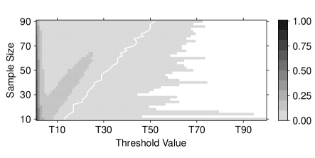
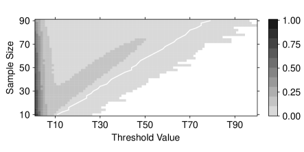
(a) (b)

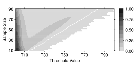
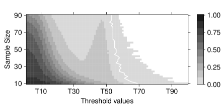
(c) (d)

(e) (f)

(g) (h)

Figure 2: Levelplot of the Core Canberra distance evaluated on the list sets $L(n,\mathcal{A},\theta,i)$. White pixels indicates experiments in which all features are discarded from all lists ($i=0$). The white line separates list sets with $i=B$ (left side) from those with $i<B$ (right side). (a)-(g): Tib500, (h): Tib100; (a): $F$, (b): mod-$F$, (c): B, (d): FC, (e): $t$, (f): mod-$t$, (g)-(h): SAM.

The group including $t$, mod-$t$, and SAM has a small number of void lists even for high thresholds, and the slope of its white line is higher: both facts indicate a not so strong dependence on the number of samples considered. On the other hand, when the same threshold is considered, the stability is higher for the group $F$, mod-$F$, and $B$. The levelplot 2d for $FC$ shows that the dependence of this methods on the dataset sample size is opposite to the behaviour of all other methods: at a given threshold, the constraint imposed gets stricter for increasing number of samples. The darker horn-shaped area in the rightmost zone of the plots is probably due to the effect that the relevant features come in groups because of the dataset definition, and this is mostly evident in the small sample sizes. As a final consideration, plots 2g and 2h show that considering the smaller dataset Tib100 instead of the larger Tib500 reflects in losing some details in the corresponding levelplot.

A few more computations and considerations on the stability of the obtained lists are shown and discussed in the following subsections.

3.2 Profiling

The second application concerns the assessment of the stability of sets of gene panels derived from profiling tasks, where different configuration of the learning scheme (e.g. the classifier, or the ranking algorithm) are compared. Here the task is how to select a list of predictive biomarkers and a classifier to predictively discriminate prostate cancer patients carrying the TMPRSS2-ER gene fusion. A basic Data Analysis Protocol (DAP for short) is applied to both cohorts of the Setlur dataset, namely a stratified 10$\times$ 5-CV, using three different classifiers: Diagonal Linear Discriminant Analysis (DLDA) [53, 54, 55, 56], linear Support Vector Machines (SVM), and Spectral Regression Discriminant Analysis (SRDA) [57]. A tuning phase through landscaping identified $10^{-3}$ as the optimal value for the SVM regularizer $C$ on both dataset, and $10^{3}$ and $10^{4}$ as the two values for the SRDA parameter $\alpha$ respectively on the US and the Sweden cohort (no tuning is needed for the DLDA classifier). Furthermore, in the SVM case the dataset is standardized to mean zero and variance one. The Entropy-based Recursive Feature Elimination (E–RFE, [58]) ranking algorithm is run on the training portion of the cross-validation split and classification models with increasing number of best ranked features are computed on the test part. The performances are evaluated at fixed feature set sizes by averaging over the CV replicates the Matthew Correlation Coefficient (MCC for short, see [59]) Eq. (4)) and the Area Under the ROC Curve (AUC for short) by using the Wilcoxon-Mann-Whitney formula Eq. (5) to extend the measure to binary classifiers. In [60, 61, 62] the equivalence with other formulations is shown: in particular, it is proved that the Wilcoxon-Mann-Whitney formula is an unbiased estimator of the classical AUC. The two performance metrics adopted have been chosen because they are generally regarded as being two of best measures in describing the confusion matrix (see Tab. 2) of true and false positives and negatives by a single number. MCC’s range is $[-1,1]$, where $MCC=0$ corresponds to the no-information error rate, which is, for a dataset with $P$ positive samples and $N$ negative samples, equivalent to $\frac{\min\{P,N\}}{P+N}$. MCC=1 is the perfect classification (FP=FN=0), while MCC=-1 denotes the worst possible performance TN=TP=0.

			Actual value
			Positive	Negative
Predicted		Positive	TP	FP
value		Negative	FN	TN

Table 2: Confusion matrix for a binary problem; T/F: true/false; TP+FN: all positive samples, TN+FP: all negative samples.

$$\textrm{MCC}=\frac{\textrm{TP}\cdot\textrm{TN}-\textrm{FP}\cdot\textrm{FN}}{\sqrt{\left(\textrm{TP}+\textrm{FP}\right)\left(\textrm{TP}+\textrm{FN}\right)\left(\textrm{TN}+\textrm{FP}\right)\left(\textrm{TN}+\textrm{FN}\right)}}\ ,$$ (4)

$$\textrm{where TN, FP, FN, TP as in Tab. \ref{tab:conf}}\ .\hfill$$

$$\textrm{AUC}=\frac{\sum_{i=1}^{n_{+}}\sum_{j=1}^{n_{-}}I(f(x^{+}_{i})>f(x^{-}_{j})}{n_{+}n_{-}}\ ,$$ (5)

$$\textrm{where $f$ classifier},\textrm{$\{x^{+}_{i}\}^{n_{+}}_{1}$ positive, $\{x^{-}_{j}\}^{n_{-}}_{1}$ negative.}\hfill$$

In Tabs. 4 and 3 we report the performances on SVM and SRDA on discrete steps of top ranked features ranging from 5 to 6144, with 95% bootstrap confidence intervals; for comparison purposes we also report AUC values for the SRDA classifier in Tab. 5. For the same values $k$ of the feature set sizes, the Canberra Core Distance is also computed on the top-$k$ ranked lists as produced by the E-RFE algorithm: the stability is also shown in the same tables. DLDA automatically choses the optimal number of features to use in order to maximize MCC (by tuning the internal parameter $nf$, starting from the default value $nf=0$), thus it is meaningless evaluating this classifier on a different feature set size. In particular, DLDA reaches maximal performances with one feature (which is the same for all replicates, DAP2_5229, leading to a zero stability value): the resulting MCC is 0.26 (CI: (0.18, 0.34)) and 0.16 (CI: 0.12, 0.19) respectively for the US and the Sweden cohort. As a reference, 5-CV with $9$-NN (which has higher performance than $k=\{5,7,11\}$) has MCC 0.36 on both cohorts with all features.

	US			Sweden
step	MCC	CI 95%	Core	MCC	CI 95%	Core
1	0.00	(0.00;0.00)	0.00	0.00	(0.00;0.00)	0.00
5	0.00	(0.00;0.00)	0.00	0.00	(0.00;0.00)	0.00
10	0.00	(0.00;0.00)	0.01	0.00	(0.00;0.00)	0.01
15	0.00	(0.00;0.00)	0.01	0.00	(0.00;0.00)	0.01
20	0.00	(0.00;0.00)	0.02	0.00	(0.00;0.00)	0.02
25	0.00	(0.00;0.00)	0.02	0.00	(0.00;0.00)	0.02
50	0.00	(0.00;0.00)	0.04	0.00	(0.00;0.00)	0.04
100	0.00	(0.00;0.00)	0.08	0.00	(0.00;0.00)	0.08
1000	0.51	(0.47;0.56)	0.52	0.08	(0.05;0.12)	0.52
5000	0.53	(0.49;0.58)	0.88	0.23	(0.20;0.27)	0.91
6144	0.53	(0.49;0.58)	0.59	0.24	(0.20;0.27)	0.62

Table 3: MCC and Core Canberra values for the two Setlur datasets for SVM classifiers.

	US			Sweden
step	MCC	CI 95%	Core	MCC	CI 95%	Core
1	0.67	(0.61;0.72)	0.00	0.40	(0.36;0.43)	0.00
5	0.55	(0.51;0.60)	0.00	0.30	(0.26;0.34)	0.00
10	0.57	(0.53;0.62)	0.01	0.33	(0.29;0.36)	0.01
15	0.57	(0.53;0.62)	0.01	0.36	(0.32;0.39)	0.01
20	0.57	(0.53;0.62)	0.02	0.39	(0.34;0.43)	0.02
25	0.57	(0.52;0.61)	0.02	0.43	(0.39;0.47)	0.02
50	0.61	(0.57;0.65)	0.04	0.44	(0.41;0.47)	0.04
100	0.59	(0.54;0.64)	0.08	0.44	(0.40;0.48)	0.08
1000	0.50	(0.45;0.55)	0.52	0.47	(0.43;0.50)	0.51
5000	0.51	(0.46;0.56)	0.89	0.46	(0.43;0.50)	0.84
6144	0.51	(0.46;0.56)	0.60	0.46	(0.42;0.49)	0.52

Table 4: MCC and Core Canberra values for the two Setlur datasets for SRDA classifiers.

	US		Sweden
step	AUC	CI 95%	AUC	CI 95%
1	0.87	(0.84;0.89)	0.79	(0.77;0.80)
5	0.83	(0.81;0.85)	0.79	(0.77;0.80)
10	0.86	(0.84;0.88)	0.80	(0.79;0.82)
15	0.88	(0.86;0.89)	0.82	(0.81;0.83)
20	0.88	(0.86;0.90)	0.83	(0.81;0.84)
25	0.89	(0.87;0.91)	0.84	(0.82;0.85)
50	0.90	(0.89;0.92)	0.84	(0.83;0.86)
100	0.90	(0.88;0.92)	0.85	(0.84;0.86)
1000	0.86	(0.85;0.88)	0.83	(0.81;0.84)
5000	0.86	(0.84;0.88)	0.82	(0.81;0.84)
6144	0.86	(0.84;0.88)	0.82	(0.81;0.84)

Table 5: AUC values for the two Setlur datasets for SRDA classifiers.

All results are displayed in the performance/stability plots of Fig. 3b. These plots can be used as a diagnostic for model selection to detect a possible choice for the optimal model as a reasonable compromise between good performances (towards the rightmost part of the graph) and good stability (towards the bottom of the graph). For instance, in the case shown we decide to use SRDA as the better classifier, using 25 features on the Sweden cohort and 10 on the US cohort: looking at the zoomed graph in Fig. 3b, if we suppose that the points are describing an ideal Pareto front, the two chosen models are the closest to the bottom right corner of the plots.

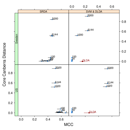
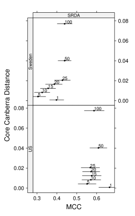
a b

Figure 3: MCC and Canberra Core values computed by using the SRDA, SVM, and DLDA models on the two Setlur datasets. Each point indicates a model with a fixed number of features, marked above the corresponding CI line.

The corresponding Borda optimal lists for SRDA models on the two Setlur datasets are detailed in Tab. 6: 5 probes are common to the two list, and, in particular, the top ranked probe is the same.

Sweden	Ranking	US	Ranking
	in US		in Sweden
DAP2_5229	1	DAP2_5229	1
DAP1_2857	5	DAP1_5091	18
DAP4_2051	3	DAP4_2051	3
DAP1_1759	13	DAP2_1680	51
DAP1_2222	19	DAP1_2857	2
DAP4_0822	44	DAP3_0905	8
DAP2_0361	403	DAP2_5769	77
DAP3_0905	6	DAP4_2271	36
DAP2_5076	24	DAP4_3958	44
DAP3_2016	16	DAP4_2442	2734
DAP4_4217	497
DAP2_0721	421
DAP4_1360	18
DAP3_1617	15
DAP1_5829	529
DAP3_6085	12
DAP4_2180	26
DAP1_5091	2
DAP1_2043	1989
DAP4_2027	2227
DAP4_1375	145
DAP4_5930	3455
DAP4_4205	25
DAP1_4950	166
DAP4_1577	283

Table 6: Borda optimal lists for SRDA models on the two Setlur datasets. In boldface, probes common to the two optimal lists. In italic, probes included in the 87-gene signature of the original paper [36]. 17 probes out of 30 are common to the 87-gene signature in [36]

In Tab. 7 we list the MCC obtained by applying the SRDA and DLDA models on the two Setlur cohorts (exchanging their role as training and test set) by using the two optimal Borda lists.

Borda	Training	Test	SRDA	DLDA
US	US	Sweden	0.39	0.44
Sweden	Sweden	US	0.42	0.48
US	Sweden	US	0.48	0.63
Sweden	US	Sweden	0.51	0.45
US	Sweden	Sweden	0.39	0.45
Sweden	US	US	0.69	0.71
US	US	US	0.71	0.78
Sweden	Sweden	Sweden	0.55	0.52

Table 7: Setlur dataset. MCC values for SRDA and DLDA optimal models.

The probe DAP2_5229 probe seems to have a relevant discriminative and predictive importance, as shown by the classwise boxplots on the two cohorts of Fig. 4. As detailed in GEO http://www.ncbi.nlm.nih.gov/geo and in NCBI Nucleotide DB http://www.ncbi.nlm.nih.gov/nuccore/, its RefSeq ID is NM_004449, whose functional description is reported as “v-ets erythroblastosis virus E26 oncogene homolog (avian) (ERG), transcript variant 2, mRNA” (information updated on 28 June 2009). In Tab. 8 we show the performances obtained by a SRDA and a DLDA model with the sole feature DAP2_5229 on all combinations of US and Sweden cohort as training and test set.

Figure 4: Boxplot of the DAP2_5229 expression value separately for the two Setlur datasets and the two class labels.

If we consider as the global optimal list the list of all 30 distinct features given as the union of the Borda list in Tab. 6, we get for SRDA and DLDA models the performances listed in Tab. 8.

		SRDA		DLDA
Training	Test	DAP2	global	DAP2	global
		5229	optimal	5229	optimal
US	Sweden	0.47	0.47	0.49	0.48
Sweden	US	0.56	0.39	0.52	0.66
Sweden	Sweden	0.50	0.55	0.39	0.56
US	US	0.68	0.73	0.68	0.76

Table 8: MCC values for SRDA and DLDA models with the only feature DAP2_5229 and with the global optimal list.

To check the consistency of the retrieved global list, we run a permutation test: we randomly extract 30 features out of the original 6144 features and we use as the p-value the number of times the obtained performances (DLDA models) are better than those obtained with the global optimal list, divided by the total number $10^{4}$ of experiments. The resulting p-values are less than $10^{-}3$ for all four combinations of using the two cohorts as training and test set, thus obtaining a reasonable significance of the global optimal list. Nevertheless if the same permutation test is run with the feature DAP2_5229 always occurring in the chosen random feature sets, the results are very different: namely, the p-value results about $0.1$, thus indicating a small statistical significance of the obtained global list. These tests seems to indicate that the occurrence of DAP2_5229 plays a key role in finding a correct predictive signature. We then performed a further experiment to detect the predictive power of the global optimal list as a function of its length. We order the global list keeping DAP2_5229, DAP4_2051, DAP1_2857, DAP3_0905, and DAP1_5091 as the first five probes and compute the performances of a DLDA model by increasing the number of features extracted from the global list from 1 to 30. The result is shown in Fig. 5: for many of the displayed models a reduced optimal list of about 10-12 features is sufficient to get almost optimal predictive performances. A permutation test on 12 features (with DAP2_5229 kept as the top probe) gives a p-value of $10^{-}2$.

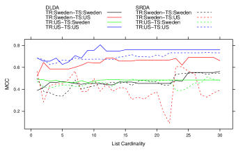
Figure 5: MCC for SRDA and DLDA models on increasing number of features extracted from the global list from 1 to 30 on the Setlur data.

A final note: our results show a slightly better AUC (in training) than the one found by the authors of the original paper [36], both in the Sweden and in the US cohort. Moreover, 17 out of 30 genes included in the global optimal list are member of the 87-gene signature shown in the original paper.

3.3 Comparing

The seven filtering algorithms of the previous subsection are also applied to the Setlur dataset, by using 100 resampling on 90% of the data on both the US and Sweden cohort separately. The Canberra Core values of the lists at different values of the filtering thresholds are shown in Fig. 6, together with a zoom on the stricter constraints area: the plots confirm the different behaviour of the groups $\{t,\textrm{mod-}t,\textrm{SAM}\}$ and $\{F,\textrm{mod-}F,\textrm{B}\}$ and of the singleton $FC$ in both cases.

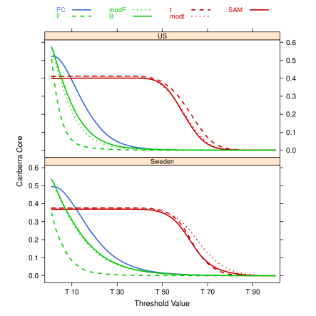
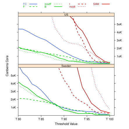
(a) (b)

Figure 6: (a): Canberra core evaluated on the Setlur dataset on B=100 repeated filtering experiments on 90% of the data. (b) Zoom on the 80%-100% threshold zone. $K=10^{5}$

By considering a cutting threshold of the 75% of the maximal value, we retrieve 14 sets of ranked partial lists, from which 14 Borda optimal lists are computed. In Tab. 9 we list the lengths of the Borda lists for each filtering method and cohort.

	F	FC	modF	modt	t	B	SAM
Sweden	1	17	25	759	326	28	366
US	1	3	6	208	367	7	149

Table 9: Length of the Borda lists for different filtering methods at 75% threshold on the Setlur dataset.

	F	FC	modF	modt	t	B	SAM	SRDA	F	FC	modF	modt	t	B	SAM	SRDA
F	$\blacksquare$	0.007	0.011	0.230	0.115	0.012	0.127	0.010	0.000	0.001	0.003	0.077	0.127	0.003	0.057	0.004
FC	122	$\blacksquare$	0.016	0.231	0.116	0.018	0.128	0.017	0.007	0.008	0.009	0.084	0.134	0.009	0.064	0.010
modF	69	129	$\blacksquare$	0.228	0.114	0.002	0.126	0.021	0.011	0.012	0.013	0.087	0.136	0.013	0.067	0.014
modt	7324	7337	7307	$\blacksquare$	0.165	0.228	0.163	0.239	0.230	0.231	0.232	0.303	0.352	0.232	0.283	0.234
t	2418	2441	2401	7379	$\blacksquare$	0.115	0.108	0.125	0.115	0.116	0.117	0.192	0.244	0.118	0.173	0.119
B	73	132	75	7308	2402	$\blacksquare$	0.127	0.022	0.012	0.013	0.014	0.088	0.138	0.014	0.068	0.016
SAM	3925	3924	3912	7287	4084	3914	$\blacksquare$	0.136	0.127	0.128	0.129	0.201	0.250	0.130	0.181	0.131
SRDA	998	1116	1067	8326	3423	1071	4916	$\blacksquare$	0.010	0.009	0.012	0.084	0.133	0.012	0.062	0.011
F	19	115	63	7317	2412	66	3919	1004	$\blacksquare$	0.001	0.003	0.077	0.127	0.003	0.057	0.004
FC	51	159	106	7360	2455	110	3962	976	55	$\blacksquare$	0.004	0.077	0.127	0.004	0.057	0.003
modF	52	111	59	7313	2408	63	3915	1049	45	88	$\blacksquare$	0.077	0.127	0.001	0.057	0.005
modt	1124	1216	1162	8393	3478	1165	4990	2032	1124	1123	1126	$\blacksquare$	0.066	0.078	0.052	0.078
t	2194	2284	2229	9449	4535	2233	6048	3070	2194	2195	2195	2081	$\blacksquare$	0.128	0.094	0.128
B	60	120	67	7321	2416	71	3923	1057	53	97	29	1126	2196	$\blacksquare$	0.058	0.006
SAM	1002	1095	1041	8283	3371	1045	4879	1843	1003	997	1004	1188	2190	1004	$\blacksquare$	0.057
SRDA	385	504	455	7711	2806	459	4311	1015	392	370	436	1406	2470	445	1241	$\blacksquare$

Table 10: Distances between Borda optimal lists (upper triangular matrix) and between all partial lists (lower triangular matrix, $\times 10^{5}$) for filtering methods (75% threshold) and SRDA models. Rows and columns 1-8 (Italic): Sweden cohort; rows and columns 9-16: US cohort.

As a first rough set-theoretical comparison, we list in Tab. 11 the probes common to more than three filtering methods. We note that only three probes are also appearing in the corresponding SRDA Borda list.

Sweden		US
gene	extractions	gene	extractions
DAP2_1768	6	DAP2_4092	5
DAP1_1949	5	DAP2_5047	5
DAP1_4198	5	DAP2_5229	5
DAP1_5095	5	DAP4_2442	5
DAP2_1037	5	DAP4_2051	4
DAP2_1151	5
DAP2_3790	5
DAP2_3896	5
DAP2_5650	5
DAP3_2164	5
DAP3_4283	5
DAP3_5834	5
DAP4_1974	5
DAP4_2316	5
DAP4_4178	5
13 genes	4

Table 11: List of probes common to more than three filtering methods

In order to get a more refined indicator of similarity, we also compute the Core Canberra Distances between all Borda optimal lists and between all 75%-threshold partial lists for filtering methods, together with the corresponding partial and Borda lists for the SRDA models: all results are reported in Tab. 10 By using the Core distances, we draw two levelplots (for both distances on Borda lists and on the whole partial lists sets, computing also a hierarchical cluster with average linkage and representing also the corresponding dendrogram in Fig. 7.

(a) (b)

Figure 7: Levelplot of the distances computed on the lists produced by filtering methods (75% threshold) and SRDA models, where the Canberra Distance is computed on (a) their Borda lists; (b) their whole list sets.

A further graphical representation of the computed distances has been obtained by using a Multidimensional Scaling (MDS) on two components, as shown in Fig. 8. On both cases, a few facts emerges: on both cohorts, the results on the Borda lists and on the whole sets of lists are similar, indicating that the Borda method is a good way to incorporate information into a single list; the behaviour grouping detected in the previous subsection is essentially confirmed here. Moreover, the two cohort are quite different, while the lists coming from the profiling experiments are not deeply different from those emerging by the filtering methods.

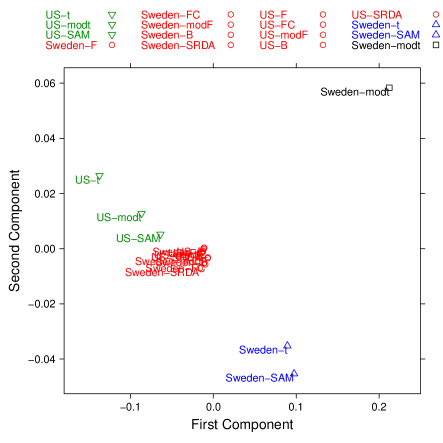
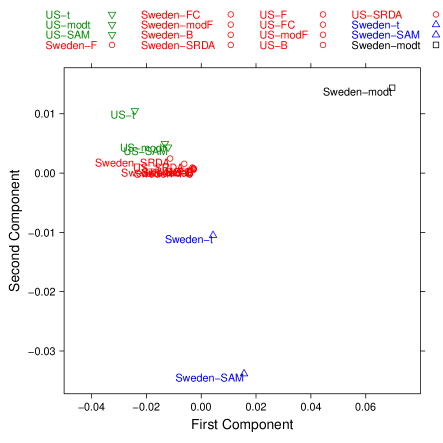
(a) (b)

Figure 8: Multidimensional Scaling (MDS) on two components computed on the lists produced by filtering methods (75% threshold) and SRDA models, where the Canberra distance is computed on (a) their Borda lists; (b) their whole list sets.

4 DISCUSSION

In [5], a correlation between signature congruency and model performance in MAQC-II [17] has been detected both in training and validation sets: the more similar the signatures, the better the average predictions.

The range of possible applications is clearly not limited to the example shown in the present work: in [1, 2, 3, 4] the importance of defining indicators for assessing ranked lists variability is discussed. At least two more applications are worth mentioning, metanalysis studies to investigate relationship between stability and classification accuracy (see for instance [17]) and analysis of lists produced by methods of gene lists enrichment.

As a final consideration, the described method may become an essential tool towards a theoretical improvement in the workfield, that is, the construction of a stability theory for feature selection, for instance in the leave-one-out stability theory already developed for classifiers [63], [64]. Attempts in this direction has been recently carried out [65], [66], [67], [68], [69], but so far no general framework has been structured yet.

5 CONCLUSIONS

In the present work, an effective method for comparing heterogeneous ranked lists coming from different experiments is shown. The algorithm is designed within the framework of the theory of metric methods for permutation groups. The introduced metric can be used in different contexts and for different purposes in many aspects of computational biology. A few examples of use are shown in the final section of the paper.

6 FUNDING

European Union (FP7 project HiperDart).

7 ACKNOWLEDGMENTS

The authors would like to thank Davide Albanese for the implementation within the mlpy package and Silvano Paoli for his support while running computation on the FBK HPC facility.

References

- [1] Boulesteix, A.-L. and Slawski, M. (2009) Stability and aggregation of ranked gene lists. Brief Bioinform, 10(5), 556–568.
- [2] Ein-Dor, L., Zuk, O., and Domany, E. (2006) Thousands of samples are needed to generate a robust gene list for predicting outcome in cancer. PNAS, 103(15), 5923–5928.
- [3] Boutros, P. C., Lau, S. K., Pintilie, M., Liu, N., Shepherd, F. A., Der, S. D., Tsao, M.-S., Penn, L. Z., and Jurisica, I. (2009) Prognostic gene signatures for non-small-cell lung cancer. PNAS, 106(8), 2824–2828.
- [4] Lau, S. K., Boutros, P. C., Pintilie, M., Blackhall, F. H., Zhu, C.-Q., Strumpf, D., Johnston, M. R., Darling, G., Keshavjee, S., Waddell, T. K., Liu, N., Lau, D., Penn, L. Z., Shepherd, F. A., Jurisica, I., Der, S. D., and Tsao, M.-S. (2007) Three-Gene Prognostic Classifier for Early-Stage Non Small-Cell Lung Cancer. J Clin Oncol, 25(35), 5562–5569.
- [5] Shi, W., Tsyganova, M., Dosymbekov, D., Dezso, Z., Nikolskaya, T., Dudoladova, M., Serebryiskaya, T., Guryanov, A., Brennan, R., Shah, R., Dopazo, J., Chen, M., Deng, Y., Shi, T., Jurman, G., Furlanello, C., Thomas, R., Corton, J., Tong, W., Shi, L., and Nikolsky, J. The Tale of Underlying biology: Functional Analysis of MAQC-II Signatures. The Tale of Underlying biology: Functional Analysis of MAQC-II Signatures., Submitted (2009).
- [6] Jurman, G., Merler, S., Barla, A., Paoli, S., Galea, A., and Furlanello, C. (2008) Algebraic stability indicators for ranked lists in molecular profiling.. Bioinformatics, 24(2), 258–264.
- [7] Critchlow, D. (1985) Metric methods for analyzing partially ranked data, LNS 34Springer, .
- [8] Diaconis, P. (1988) Group representations in probability and statistics, Institute of Mathematical Statistics Lecture Notes – Monograph Series 11IMS, .
- [9] Lance, G. and Williams, W. (1967) Mixed-Data Classificatory Programs I - Agglomerative Systems. Aust. Comput. J., 1(1), 15–20.
- [10] Jurman, G., Riccadonna, S., Visintainer, R., and Furlanello, C. . (2009) Canberra Distance on Ranked Lists. In Agrawal, S., Burges, C., and Crammer, K., (eds.), Proceedings of Advances in Ranking NIPS 09 Workshop, pp. 22–27.
- [11] Gobbi, A. Algebraic and combinatorial techniques for stability algorithms on ranked data. Master’s thesis University of Trento (2008).
- [12] Fagin, R., Kumar, R., and Sivakumar, D. (2003) Comparing top- lists. SIAM J. Disc. Math., 17(1), 134–160.
- [13] Bar-Ilan, J., Mat-Hassan, M., and Levene, M. (2006) Methods for comparing rankings of search engine results. Comput. Netw., 50(10), 1448–1463.
- [14] Fury, W., Batliwalla, F., Gregersen, P., and Li, W. (2006) Overlapping Probabilities of Top Ranking Gene Lists, Hypergeometric Distribution, and Stringency of Gene Selection Criterion. In IEEE, (ed.), 28th IEEE EMBS Ann. Intl. Conf., New York City, USA, pp. 5531–5534.
- [15] Pearson, R. (2007) Reciprocal rank-based comparison of ordered gene lists. In IEEE, (ed.), IEEE Intl. Workshop on Genomic Signal Processing and Statistics, 2007. GENSIPS 2007, pp. 1–3.
- [16] Yang, X. and Sun, X. (2007) Meta-analysis of several gene lists for distinc types of cancer: A simple way to reveal common prognostic markers. BMC Bioinf., 8, 118.
- [17] The MicroArray Quality Control (MAQC) Consortium The MAQC-II Project: A comprehensive study of common practices for the development and validation of microarray-based predictive models. The MAQC-II Project: A comprehensive study of common practices for the development and validation of microarray-based predictive models., Submitted (2009).
- [18] Kendall, M. (1962) Rank correlation methods, Griffin Books on StatisticsGriffin & Co., London, .
- [19] Diaconis, P. and Graham, R. (1977) Spearman’s Footrule as a Measure of Disarray. J. R. Stat. Soc. B, 39, 262–268.
- [20] Graham, R., Knuth, D., and Patashnik, O. (1989) Concrete Mathematics: A Foundation for Computer Science, Addison Wesley, Reading, Mass., .
- [21] Cheon, G.-S. and El-Mikkawy, M. E.-A. (2007) Generalized Harmonic Number Identities And Related Matrix Representation. J. Korean Math. Soc., 44(2), 487–498.
- [22] Simić, S. (1998) Best possible bounds and monotonicity of segments of harmonic series (II). Matematicki Vesnik, 50, 5–10.
- [23] Villarino, M. Ramanujan’s Approximation to the -th Partial Sum of the Harmonic Series. Ramanujan’s Approximation to the -th Partial Sum of the Harmonic Series., Preprint: arXiv:math.CA/0402354 v5 (2004).
- [24] Villarino, M. Sharp Bounds for the Harmonic Numbers. Sharp Bounds for the Harmonic Numbers., Preprint: arXiv:math.CA/0510585 v3 (2006).
- [25] Kauers, M. and Schneider, C. (2006) Indefinite Summation with Unspecified Summands. Discrete Math., 306(17), 2021–2140.
- [26] Kauers, M. and Schneider, C. (2006) Application of Unspecified Sequences in Symbolic Summation. In ACM, (ed.), Proceedings of the 2006 International Symposium on Symbolic and Algebraic Computation, pp. 177–183.
- [27] Schneider, C. (2004) Symbolic Summation with Single-Nested Sum Extension. In ACM, (ed.), Proceedings of the 2004 International Symposium on Symbolic and Algebraic Computation, pp. 282–289.
- [28] Abramov, S., Carette, J., Geddes, K., and Lee, H. (2004) Telescoping in the context of symbolic summation in Maple. J. Symb. Comput., 38, 1303–1326.
- [29] Schneider, C. (2007) Simplifying Sums in -Extensions. J. Algebra Appl., 6(3), 415–441.
- [30] Hoeffding, W. (1951) A Combinatorial Central Limit Theorem. Ann. Math. Stat., 22(4), 558–566.
- [31] Borda, J. (1781) Mémoire sur les élections au scrutin. Histoire de l’Académie Royale des Sciences, Année MDCCLXXXI.
- [32] Saari, D. (2001) Chaotic Elections! A Mathematician Looks at Voting, AMS, .
- [33] Albanese, D., Merler, S., Jurman, G., Visintainer, R., and Furlanello, C. mlpy: High-performance Python ackage for predictive modeling. NIPS Workshop: Machine Learning Open Source Software (2008) http://videolectures.net/mloss08\_albanese\_mlp/.
- [34] Albanese, D., Visintainer, R., Jurman, G., Merler, S., Riccadonna, S., Paoli, S., Chierici, M., and Furlanello, C. mlpy: a Python package for machine learning. mlpy: a Python package for machine learning., In preparation (2009).
- [35] Bair, E. and Tibshirani, R. (2004) Semi–supervised methods to predict patient survival from gene expression data. PLOS Biol., 2(4), 511–522.
- [36] Setlur, S., Mertz, K., Hoshida, Y., Demichelis, F., Lupien, M., Perner, S., Sboner, A., Pawitan, Y., Andrén, O., Johnson, L., Tang, J., Adami, H., Calza, S., Chinnaiyan, A., Rhodes, D., Tomlins, S., Fall, K., Mucci, L., Kantoff, P., Stampfer, M., Andersson, S., Varenhorst, E., Johansson, J., Brown, M., Golub, T., and Rubin, M. (2008) Estrogen-dependent signaling in a molecularly distinct subclass of aggressive prostate cancer. J. Natl. Cancer Inst., 100(11), 815–825.
- [37] Yao, C., Zhang, M., Zou, J., Gong, X., Zhang, L., Wang, C., and Guo, Z. (2008) Disease prediction power and stability of differential expressed genes. In IEEE, (ed.), 2008 Intl. Conf. BioMedical Engineering and Informatics, pp. 265–268.
- [38] Chen, J., Hsueh, H.-M., Delongchamp, R., Lin, C.-J., and Tsai, C.-A. (2007) Reproducibility of microarray data: a further analysis of microarray quality control (MAQC) data. BMC Bioinf., 8, 412.
- [39] Simon, R. (2008) Microarray-based expression profiling and informatics. Curr. Opin. Biotechnol., 16, 26–29.
- [40] Tusher, V., Tibshirani, R., and Chu, G. (2001) Significance analysis of microarrays applied to the ionizing radiation response. PNAS, 98, 5116–5121.
- [41] Storey, J. (2002) A direct approach to false discovery rates. J. Roy. Stat. Soc. Ser. B, 64, 479–498.
- [42] Efron, B., Tibshirani, R., Storey, J., and Tusher, V. (2001) Empirical Bayes Analysis of a Microarray Experiment. JASA, 96, 1151–1160.
- [43] Efron, B. and Tibshirani, R. (2002) Empirical Bayes Methods, and False Discovery Rates. Genet. Epidemiol., 23(1), 70–86.
- [44] Efron, B., Tibshirani, R., and Taylor, J. (2005) The “Miss rate” for the analysis of gene expression data. Biostat., 6(1), 111–117.
- [45] Witten, D. and Tibshirani, R. A comparison of fold-change and the t-statistic for microarray data analysis. Technical report Department of Statistics, Stanford University (2007) http://www-stat.stanford.edu/~tibs/ftp/FCTComparison.pdf.
- [46] Jeffery, I., Higgins, D., and Culhane, A. (2006) Comparison and evaluation of methods for generating differentially expressed gene lists from microarray data. BMC Bioinf., 7, 359.
- [47] Lönnstedt, I. and Speed, T. (2001) Replicated microarray data. Stat. Sinica, 12(1), 31–46.
- [48] Neter, J., Kutner, M., Nachtsheim, C., and Wasserman, W. (1996) Applied Linear Statistical Models, McGraw-Hill/Irwin, .
- [49] Smyth, G. (2003) Linear models and empirical bayes methods for assessing differential expression in microarray experiments. Stat. Appl. Genet. Mol. Biol., 3, Article 3.
- [50] Xiao, Y. and Yang, Y. H. Bioconductor’s DEDS package (2008).
- [51] Gentleman, R., Carey, V., Bates, D., Bolstad, B., Dettling, M., Dudoit, S., Ellis, B., Gautier, L., Ge, Y., Gentry, J., Hornik, K., Hothorn, T., Huber, W., Iacus, S., Irizarry, R., Leisch, F., Li, C., Maechler, M., Rossini, A. J., Sawitzki, G., Smith, C., Smyth, G., Tierney, L., Yang, J., and Zhang, J. (2004) Bioconductor: Open software development for computational biology and bioinformatics. Genome Biol., 5, R80.
- [52] R Development Core Team R: A Language and Environment for Statistical Computing R Foundation for Statistical Computing Vienna, Austria (2008) ISBN 3-900051-07-0.
- [53] Pique-Regi, R. and Ortega, A. (2006) Block diagonal linear discriminant analysis with sequential embedded feature selection. In IEEE, (ed.), ICASSP 2006, IEEE International Conference on Acoustics, Speech and Signal Processing, Vol. 5, .
- [54] Pique-Regi, R., Ortega, A., and Asgharzadeh, S. (2005) Sequential Diagonal Linear Discriminant Analysis (SeqDLDA) for Microarray Classification and Gene Identification. In IEEE, (ed.), CSBW ’05, IEEE Computational Systems Bioinformatics Conference - Workshops, pp. 112–116.
- [55] Bø, T. and Jonassen, I. (2002) New feature subset selection procedures for classification of expression profiles. Genome Biol., 3(4), research0017.1–research0017.11.
- [56] Dudoit, S., Fridlyand, J., and Speed, T. (2002) Comparison of Discrimination Methods for the Classification of Tumors Using Gene Expression Data. J. Am. Stat. Assoc., 97, 77–87.
- [57] Cai, D., Xiaofei, H., and Han, J. (2008) Srda: An efficient algorithm for large-scale discriminant analysis. IEEE Transactions on Knowledge and Data Engineering, 20(1), 1–12.
- [58] Furlanello, C., Serafini, M., Merler, S., and Jurman, G. (2003) Entropy-Based Gene Ranking without Selection Bias for the Predictive Classification of Microarray Data. BMC Bioinformatics, 4(1), 54.
- [59] Baldi, P., Brunak, S., Chauvin, Y., Andersen, C., and Nielsen, H. (2000) Assessing the accuracy of prediction algorithms for classification: an overview. Bioinformatics, 16(5), 412–424.
- [60] Cortes, C. and Mobri, M. (2003) AUC optimization vs. error rate minimization. In Thrun, S., Saul, L., and Schölkopf, B., (eds.), Advances in Neual Information Processing Systems 16 (NIPS 2003), Vancouver, BC, Canada, December 8-13, 2003, Cambridge: MIT Press Vol. 16, pp. 169–176.
- [61] Calders, T. and Jaroszewicz, S. (2007) Efficient AUC Optimization for Classification. In Springer-Verlag, (ed.), PKDD 2007: Proceedings of the 11th European conference on Principles and Practice of Knowledge Discovery in Databases, Warsaw, Poland, Berlin, Heidelberg: pp. 42–53.
- [62] Vanderlooy, S. and Hüllermeier, E. (2008) A critical analysis of variants of the AUC. Machine Learning, 72(3), 247–262.
- [63] Mukherjee, S., Niyogi, P., Poggio, T., and Rifkin, R. (2006) Learning theory: stability is sufficient for generalization and necessary and sufficient for consistency of empirical risk minimization. Advances in Computational Mathematics, 25, 161–193.
- [64] Bousquet, O. and Elisseeff, A. (2002) Stability and generalization. Journal of Machine Learning Research, 2, 499–526.
- [65] Kalousis, A., Prados, J., and Hilario, M. (2005) Stability of feature selecion algorithms. In IEEE, (ed.), ICDM’05: Proceedings of the Fifth IEEE International Conference on Data Mining (ICNC 2007), pp. 218–225.
- [66] Kuncheva, L. (2007) A stability index for feature selecion. In Press, A., (ed.), Proceedings of the 25th conference on Proceedings of the 25th IASTED International Multi-Conference: artificial intelligence and applications, pp. 390–395.
- [67] Zhang, L. (2007) A Method for Improving the Stability of Feature Selection Algorithm. In IEEE, (ed.), ICNC ’07: Proceedings of the Third International Conference on Natural Computation (ICNC 2007), Washington, DC, USA: pp. 715–717.
- [68] Kr̆íz̆ek, P., Kittler, J., and Hlavác̆, V. (2007) Improving Stability of Feature Selection Methods. In Kropatsch, W., Kampel, M., and Hanbury, A., (eds.), CAIP 2007, Computer Analysis Image Processing, pp. 929–936.
- [69] Xiao, Y., Hua, J., and Dougherty, E. R. (2007) Quantification of the impact of feature selection on the variance of cross-validation error estimation. Journal of Bioinformatics and Systems Biology, 2007.