Swimming microorganisms Fluid transport and rheology Physiological materials

Low-Reynolds number swimming in gels

Abstract

Many microorganisms swim through gels, materials with nonzero zero-frequency elastic shear modulus, such as mucus. Biological gels are typically heterogeneous, containing both a structural scaffold (network) and a fluid solvent. We analyze the swimming of an infinite sheet undergoing transverse traveling wave deformations in the “two-fluid” model of a gel, which treats the network and solvent as two coupled elastic and viscous continuum phases. We show that geometric nonlinearities must be incorporated to obtain physically meaningful results. We identify a transition between regimes where the network deforms to follow solvent flows and where the network is stationary. Swimming speeds can be enhanced relative to Newtonian fluids when the network is stationary. Compressibility effects can also enhance swimming velocities. Finally, microscopic details of sheet-network interactions influence the boundary conditions between the sheet and network. The nature of these boundary conditions significantly impacts swimming speeds.

While biological locomotion at low-Reynolds number is a well-established and active field (see [1] for a review), only recently has swimming in complex, non-Newtonian media started to be systematically explored. Indeed, many microorganisms routinely swim through complex or non-Newtonian media. Bacteria in the stomach such as Helicobacter pylori encounter gastric mucus [2]; mammalian sperm swim through viscoelastic mucus in the female reproductive tract [3, 4]; and spirochetes burrow into the tissues they infect [5]. Most of the prior theoretical work on swimming in complex media has focused on viscoelastic fluids [6, 7, 8, 9, 10, 11, 12, 13, 14]. Because prescribed swimming strokes lead to the same swimming speed in linearly viscoelastic fluids as in Newtonian fluids [7, 13], these studies have focused on the effects of nonlinear viscoelasticity [6, 8, 9, 11, 12, 13, 14] and the effect of altered medium response on swimming strokes via fluid-structure interactions [9, 10]. However, many biological viscoelastic materials contain crosslinked polymer networks, and are therefore solid rather than fluid. In this paper we focus on swimming in such crosslinked materials, which have a nonzero zero-frequency elastic shear modulus. We use the term “gel” to refer to these types of materials.

Generally, viscoelastic materials have frequency-dependent response, while the distinction we make between solid and fluid is a zero-frequency property. Some of the issues addressed by studies of viscoelastic fluids carry over straightforwardly to gels. For example, the fluid-structure interactions which determine the beating patterns of sperm flagella depend on the viscoelastic response at the beating frequency, not at zero frequency. However, a simple physical argument demonstrates a fundamental difference between swimming in a gel versus swimming in a fluid. In fluid dynamics, one uses no-slip boundary conditions, but for a swimmer in a solid, no-slip boundary conditions do not allow swimming. Under no-slip boundary conditions a swimmer would drag solid material along with its motion, leading to large deformations and restoring forces which oppose translation. Thus, swimming in a gel requires that the swimmer slips past the medium. This simple consideration highlights the importance of boundary conditions for understanding swimming in gels, a major theme of this paper.

Another motivation for studying swimming in gels is the search for mechanisms that enhance swimming speeds in complex materials. Due to the observation that spirochetes can swim faster in fluids with an elastic response component [15], there has been an interest in how viscoelastic media can increase or decrease swimming velocities. For filamentous geometries, it has been suggested that polymeric fluids may have higher effective anisotropies in resistive-force theories, leading to increased swimming speeds [16, 17]. Furthermore, the breaking of kinematic reversibility [18] in nonlinearly viscoelastic fluids makes certain reciprocal swimming strokes more effective than in Newtonian fluids [11, 13]. Restricting attention to sheet-like geometries undergoing traveling-wave deformations (the subject of this paper), an infinite sheet in a nonlinearly viscoelastic fluids swims more slowly than in a Newtonian medium [8]. However, finite-length sheet-like swimmers in viscoelastic fluids [14], and infinite swimmers in a Brinkmann fluid can show increased swimming velocities [19, 17].

The latter two studies [19, 17] are closest in spirit to this letter. Both investigate how Taylor’s swimming sheet [20], an infinite sheet with a small amplitude traveling wave deformation, behaves in the Brinkmann model, which treats the effect of a stationary porous phase on fluid flows in an effective medium approach. Instead, we solve for the flows induced by the moving sheet in the “two-fluid model” description of a gel [21, 22, 23, 24], which represents the gel as two phases. One phase describes an elastic polymer network with displacement field $\mathbf{u}$ and Lamé coefficients $\mu$ and $\lambda$, and the other phase describes a viscous fluid solvent with velocity field $\mathbf{v}$ and viscosity $\eta$. The two phases are coupled by a drag force proportional to their relative local velocity, with drag coefficient $\Gamma$, giving the governing equations

$$\nabla\cdot{\bm{\sigma}}^{\mathrm{n}} = \Gamma\left(\frac{\mathrm{d}}{\mathrm{d}t}{\mathbf{u}}-\mathbf{v}\right)$$ (1)

$$\nabla\cdot{\bm{\sigma}}^{\mathrm{s}} = -\Gamma\left(\frac{\mathrm{d}}{\mathrm{d}t}{\mathbf{u}}-\mathbf{v}\right)$$ (2)

$$\bm{\sigma}^{\mathrm{n}} = \mu\left[\nabla\mathbf{u}+(\nabla\mathbf{u})^{\mathrm{T}}\right]+\mathbf{I}\;\lambda\nabla\cdot\mathbf{u}+\bm{\bar{\sigma}}^{\mathrm{n}}$$ (3)

$$\bm{\sigma}^{\mathrm{s}} = \eta\left[\nabla\mathbf{v}+(\nabla\mathbf{v})^{\mathrm{T}}\right]-p\;\mathbf{I}$$ (4)

$$-\partial_{t}\varphi = \nabla\cdot\left[\varphi\frac{\mathrm{d}}{\mathrm{d}t}\mathbf{u}\right]$$ (5)

$$-\partial_{t}(1-\varphi) = \nabla\cdot\left[(1-\varphi)\mathbf{v}\right].$$ (6)

Here the network and solvent stress tensors are $\bm{\sigma}^{\mathrm{n}}$ and $\bm{\sigma}^{\mathrm{s}}$, respectively. The moduli in the network stress tensor are effective, macroscopic moduli – for example, they incorporate osmotic effects, and they depend implicitly on the volume fraction of the network. Eq. 5 and 6 express volume conservation for each phase in terms of the network volume fraction $\varphi$ assuming that the individual solvent and network phases are incompressible. Combining the two yields

$$0=\nabla\cdot\left[(1-\varphi)\mathbf{v}+\varphi\frac{\mathrm{d}}{\mathrm{d}t}\mathbf{u}\right].$$ (7)

In the rest of the paper, we work in the regime where network volume fraction $\varphi$ can be ignored, but yet the macroscopic network stresses cannot be ignored, i.e. if we expand the solutions in $\varphi$, we obtain the zeroth-order solutions in $\varphi$. In this $\varphi\rightarrow 0$ limit, Eq. 7 reduces to $\nabla\cdot\mathbf{v}=0.$ The drag coefficient $\Gamma$ can be estimated as $\Gamma\approx\eta/\xi^{2}$, where $\xi$ is the mesh size of the network [21]. Finally, note that the network stress tensor incorporates nonlinear terms (involving products of $\mathbf{u}$) explicitly in $\bar{\bm{\sigma}}^{\mathrm{n}}$.

Our use of the two-fluid model explicitly recognizes the role of heterogeneity in complex media, while still retaining a continuum description. Ref. [17] emphasizes that polymers in a viscoelastic fluid may be viewed as heterogeneous inclusions in a viscous fluid. Treating the inclusions as a stationary background results in the Brinkmann fluid as an effective model. The two-fluid model allows us to describe the heterogeneous phase more realistically as a dynamic component, and understand when it is appropriate to think of heterogeneities as stationary or dynamic.

Our investigation leads to three main conclusions. First, network dynamics determine when the presence of heterogeneities leads to increased swimming velocities. Roughly speaking, network deformations are a result of drag forces arising from solvent flow, and are opposed by the stiffness of the network. For fast flows or compliant networks, the networks move with the flows and do not attenuate the flow, while for slow flows or stiff networks, the network acts like a stationary phase, leading to enhancements of the swimming velocity. We also find that compressibility of the network can lead to additional enhancement of swimming velocities.

Second, a consistent treatment of swimming velocities requires proper treatment of nonlinearities. We show that nonlinearities in the constitutive relationship ($\bar{\bm{\sigma}}^{\mathrm{n}}$ in Eq. 3) of the elastic phase of a gel do not affect swimming speeds. However, geometric nonlinearities arise from the terms of Eqs. 1 and 2 that involve the velocity of material points of the network, $\frac{\mathrm{d}}{\mathrm{d}t}\mathbf{u}$. The displacement field is a function of current coordinates – i.e., the position of a material element originally at $\mathbf{x}_{0}$ is $\mathbf{x}(\mathbf{x}_{0},t)=\mathbf{x}_{0}+\mathbf{u}(\mathbf{x},t)$ – so the velocity of material elements is given by the material derivative, defined implicitly via $\frac{\mathrm{d}}{\mathrm{d}t}\mathbf{u}=\partial_{t}{\mathbf{u}}+\frac{\mathrm{d}}{\mathrm{d}t}\mathbf{u}\cdot\nabla\mathbf{u}$. In the remainder of the paper we refer to the term $\frac{\mathrm{d}}{\mathrm{d}t}\mathbf{u}\cdot\nabla\mathbf{u}$ as the “convective” nonlinearity. Without it one cannot obtain physically meaningful swimming velocities.

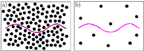
Figure 1: Effective sheet-network boundary conditions depend on the microscopic swimmer-network interactions. a) Network is dense on the scale of swimmer deformations leading to direct network-sheet boundary conditions (Eqs. 8 and 9). b) Network is sparse on the scale of swimmer deformations leading to solvent-mediated network-sheet boundary conditions (Eq. 10).

Finally, we highlight the importance of boundary conditions (BC) between the sheet and elastic phase. There is a long history of experimental support for the validity of no-slip boundary conditions for fluids, and we use no-slip BC between the sheet and solvent, $\mathbf{v}(x,h(x,t),t)=\partial_{t}h(x,t)\hat{\bf{y}}$, where $h(x,t)$ is height of the sheet at $(x,t)$. However, there is no a priori selection of boundary conditions between the sheet and network in our macroscopic theory. In this paper, we consider two types of network-sheet BC that may plausibly result from microscopic interactions at a swimmer surface.

The first class of boundary conditions applies when the network is dense on the scale of the swimmer (Fig. 1a). Then we imagine that the sheet presses directly against the polymer network and the network must conform to the sheet. Using reference positions for the network produced by a flat sheet,

$$u_{y}(x,h(x,t),t)=h(x,t).$$ (8)

The remaining boundary condition is applied to the tangential network stress via a kinetic friction law, with tangential stress proportional to the tangential velocity of the polymer relative to the sheet:

$$\hat{\bf t}\cdot\bm{\sigma}^{\mathrm{n}}(x,h(x,t),t)\cdot\hat{\bf n}=$$ (9)

$$\!\!\!\!\!\!\!\!\!\!\!\!\!\!\!\!\!\!\!\!\!\!\!\!\!\!\!\!\!\!\!\Xi\hat{\bf t}\cdot\left(\frac{\mathrm{d}}{\mathrm{d}t}{\mathbf{u}}(x,h(x,t),t)-\partial_{t}h(x,t)\hat{\bf{y}}\right),$$

where $\hat{\bf t}$ and $\hat{\bf n}$ are the tangent and normal to the sheet. Note that $\Xi\rightarrow 0$ corresponds to free tangential slip, while $\Xi\rightarrow\infty$ corresponds to no-slip.

In the second class of boundary condition, the network is dilute on the scale of the swimmer (Fig. 1b), so the sheet exerts no forces directly on the network. Instead all forces on the network are mediated by the solvent. Then the two components of the network stress acting on the sheet must vanish:

$$\bm{\sigma}^{\mathrm{n}}(x,h(x,t),t)\cdot\hat{\bf n}=0.$$ (10)

Both the “direct” BC (Eqs. 8,9) and “solvent-mediated” BC (Eq. 10) allow the swimmer to slide past the network, in accordance with our physical discussion above.

Solutions. In the frame where the sheet is stationary, the transverse displacements are described by $h(x,t)=\mathrm{Re}[b\exp(i(kx-\omega t)]$. Throughout this paper we will be concerned with the zero-Reynold’s number limit appropriate for swimming microorganisms, and hence always ignore inertial effects.

The sheet swims with velocity $V_{s}$, but sufficiently far from the sheet in the lab frame the elastic phase is stationary. Thus we write the displacement field in the frame of the sheet as $\mathbf{u}(\mathbf{x},t)=V_{s}\,t\,\hat{\bf x}+\delta\mathbf{u}(\mathbf{x},t)$, with $\delta\mathbf{u}$ small. Note that $V_{s}$ turns out to be second order in the displacements. The solution strategy follows Taylor [20]. For small traveling wave amplitudes relative to wavelengths, we determine the velocity and displacement fields order by order in $b$. We write (for example) $\delta\mathbf{u}=\delta\mathbf{u}^{(1)}+\delta\mathbf{u}^{(2)}+...$, with $\delta\mathbf{u}^{(1)}$ first order in $b$, etc. The fields satisfy the governing equations and boundary conditions, also expanded order by order in $b$.

The first-order governing equations are

$$\mu\nabla^{2}\delta\mathbf{u}^{(1)}+(\lambda+\mu)\nabla(\nabla\cdot\delta\mathbf{u}^{(1)}) = \Gamma\left(\partial_{t}\delta\mathbf{u}^{(1)}-\mathbf{v}^{(1)}\right)$$

$$\eta\nabla^{2}\mathbf{v}^{(1)}-\nabla p = -\Gamma\left(\partial_{t}\delta\mathbf{u}^{(1)}-\mathbf{v}^{(1)}\right).$$

The first-order solutions take the form $\mathbf{v}^{(1)}=\mathrm{Re}\{\tilde{\mathbf{v}}(y)\exp(i(kx-\omega t))\}$ (for example). The first order solutions can be found by introducing stream and potential functions, $\mathbf{v}^{(1)}=\mathrm{curl}(\Psi\hat{\mathbf{z}})$ and $\delta\mathbf{u}^{(1)}=\mathrm{curl}(\Phi\hat{\mathbf{z}})+\nabla\chi$, and then following the methods detailed in  [24]. Once the first order solutions are obtained, the swimming velocity is found by solving the second order equations. The swimming velocity is determined by $x$-component of the time- and $x$-averaged velocity and displacement fields. Note that any overall time- or $x$-derivative vanishes upon averaging, so the time-averaged $x$-components of the 2nd order pieces of Eq. 1 and 2 are

$$-\eta\partial_{y}^{2}\langle v_{x}^{(2)}\rangle = \mu\partial_{y}^{2}\langle\delta u_{x}^{(2)}\rangle+\partial_{y}\langle\bar{\sigma}^{{\mathrm{n}}(2)}_{yx}\rangle$$ (11)

$$\!\!\!\!\!\!\!\!\!\!\!\!\!\!\!\!\!\!\!\!\!\!\!\!=\Gamma[V_{s}-\langle v_{x}^{(2)}\rangle+\langle(\partial_{t}\delta\mathbf{u}^{(1)}\cdot\nabla)\delta u_{x}^{(1)}\rangle].$$

Here the brackets denote time-and x-averaging and $\bar{\sigma}^{{\mathrm{n}}(2)}_{yx}$ includes the 2nd order contributions to the network stress involving products of two first order fields. The solutions to these second order equations are $\langle v_{x}^{(2)}\rangle=V_{s}+c_{1}\exp(-\sqrt{\Gamma/\eta}y)+f(y)$ and $\langle\delta u_{x}^{(2)}\rangle=-(\eta/\mu)\langle v_{x}^{(2)}\rangle+g(y)$, where $f(y)$ is the inhomogeneous solution satisfying $(\eta\partial_{y}^{2}-\Gamma)f=-\Gamma\langle\partial_{t}\delta\mathbf{u}^{(1)}\cdot\nabla\delta u_{x}^{(1)}\rangle$ and $g(y)$ is the inhomogeneous solution satisfying $\mu\partial_{y}g=-\langle\bar{\sigma}_{xy}^{{\mathrm{n}}(2)}\rangle$. Boundary conditions at infinity rule out other possible solutions.

These solutions must satisfy the second order boundary conditions, obtained by expanding Eqs. 9 and 10 using $\hat{\mathbf{n}}\approx\hat{\mathbf{y}}-\partial_{x}h\hat{\mathbf{x}}$ and $\hat{\mathbf{t}}\approx\hat{\mathbf{x}}+\partial_{x}h\hat{\mathbf{y}}$. For direct sheet-network interactions, the relevant BC are

$$\mathrm{see~{}Eqs.~{}\ref{V2BC}~{}and~{}\ref{U2BC}}$$

$$\langle v_{x}^{(2)}\rangle = -\langle h\partial_{y}v_{x}^{(1)}\rangle$$ (12)

$$\left(\begin{array}[]{c}\mu\partial_{y}\langle\delta u_{x}^{(2)}\rangle+\langle\bar{\sigma}_{xy}^{{\mathrm{n}}(2)}\rangle+\langle h\partial_{y}\sigma_{xy}^{{\mathrm{n}}(1)}\rangle\\ +\langle\partial_{x}h\sigma_{yy}^{{\mathrm{n}}(1)}\rangle-\langle\partial_{x}h\sigma_{xx}^{{\mathrm{n}}(1)}\rangle\end{array}\right) = \Xi\left(\begin{array}[]{c}V_{s}+\langle\partial_{t}{\delta\mathbf{u}}^{(1)}\cdot\nabla\delta u^{(1)}_{x}\rangle\\ +\langle h\partial_{y}\partial_{t}{\delta u_{x}}^{(1)}\rangle+\langle\partial_{t}{\delta u_{y}}^{(1)}\partial_{x}h\rangle-\langle\partial_{t}h\partial_{x}h\rangle\end{array}\right),$$ (17)

with all quantities evaluated at $y=0$. Eqs. 12 and 17 also apply for solvent-mediated BC, provided that we set $\Xi=0$ in Eq. 17. In Eq. 17, note that all pieces involving $\langle\bar{\sigma}_{xy}^{{\mathrm{n}}(2)}\rangle$ cancel due to the form of $\langle\delta u_{x}^{(2)}\rangle$. Therefore nonlinearities in the constitutive relation for the polymer stress (i.e., $\bar{\bm{\sigma}}^{\mathrm{n}}$) do not affect the swimming velocity at second order. Similar cancellations help to show that these solutions satisfy overall force balance on the swimmer.

Eliminating $c_{1}$ from Eqs. 12 and 17 yields $V_{s}$ in terms of first order quantities. For direct network-sheet BC,

$$\mathrm{see~{}Eq.~{}\ref{swimspeed}}$$

$$V_{s}=-{\left(1+\frac{\sqrt{\Gamma\eta}}{\Xi}\right)^{-1}}{\left(\begin{array}[]{c}\left(-\langle\partial_{t}h\partial_{x}h\rangle+\langle h\partial_{y}\partial_{t}{\delta u_{x}}^{(1)}\rangle+\langle\partial_{t}{\delta u_{y}}^{(1)}\partial_{x}h\rangle+\langle\partial_{t}{\delta\mathbf{u}}^{(1)}\cdot\nabla\delta u^{(1)}_{x}\rangle\right)\\ +\frac{\sqrt{\Gamma\eta}}{\Xi}\left(\langle h\partial_{y}v_{x}^{(1)}\rangle+f(0)\right)+\frac{\eta}{\Xi}\partial_{y}f(0)-\frac{1}{\Xi}\left(\langle h\partial_{y}\sigma_{xy}^{{\mathrm{n}}(1)}\rangle+\langle\partial_{x}h(\sigma_{yy}^{{\mathrm{n}}(1)}-\sigma_{xx}^{{\mathrm{n}}(1)})\rangle\right)\end{array}\right)}.$$ (18)

The fourth term on the right hand side, $\langle\partial_{t}{\delta\mathbf{u}}^{(1)}\cdot\nabla\delta u^{(1)}_{x}\rangle$, arises from the convective nonlinearity. For the solvent-mediated BC, the swimming velocity is given by Eq. 18 with $\Xi=0$. However, the swimming velocity with solvent-mediated BC is not just the swimming velocity with direct BC for $\Xi=0$, since the first-order solutions differ.

For an incompressible network ($\lambda\rightarrow\infty$) the swimming velocity has a simple form when the convective nonlinearity is included:

$$V_{s}=b^{2}\omega k\frac{\sqrt{\Gamma\eta}[4+6\sqrt{\Gamma/(\eta k^{2})}+\Gamma/(\eta k^{2})]}{(\Xi+\sqrt{\Gamma\eta})[2+\sqrt{\Gamma/(\eta k^{2})}]^{3}}.$$ (19)

For an incompressible network the swimming velocity is the same as in a Newtonian fluid, $V_{N}=b^{2}\omega k/2$, when the convective nonlinearity is not included.

Results and discussion. Our solutions reveal that the heterogeneous nature of gels leads to behavior not captured by modeling viscoelastic media as single-phase fluids. This is apparent even in the first order solutions. In a viscoelastic fluid, the first order solutions are the same as in a Newtonian fluid, while in our solutions, once the network becomes compressible, or once one uses solvent-mediated sheet-network BC, there is relative motion between the solvent and network and both phases move differently from a Newtonian fluid.

Turning to the swimming velocities, we see the importance of correctly accounting for nonlinearities. As in previous studies of the role of nonlinearities in single-phase viscoelastic fluids [8, 9, 11], for small amplitude swimming strokes the swimming speed is a second order effect, and so a consistent description must take into account any nonlinearities in constitutive laws. In the case of a gel described using a two-fluid model, we have shown that for both direct and solvent-mediated sheet-network BC, nonlinearities in the constitutive law for the elastic phase do not affect the swimming velocity. However, the geometric convective nonlinearity must be taken into account to obtain physically meaningful swimming velocities. Fig. 2 shows the swimming velocity as a function of inverse friction $1/\Xi$. Previously we argued that no-slip sheet-network BC prevent a sheet from swimming, which implies that the swimming velocity should vanish as $1/\Xi\rightarrow 0$, (the no-slip limit). The figure shows that this expected behavior is only obtained when the convective nonlinearities are included. This holds for incompressible networks ($\lambda\rightarrow\infty$) as well as stiff (small $\eta\omega/\mu$) and compliant (large $\eta\omega/\mu$) compressible networks. In the rest of this paper we always include the convective nonlinearity.

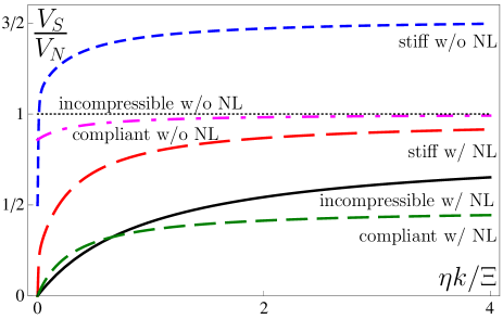
Figure 2: Swimming speed normalized by Newtonian swimming speed, $V_{s}/V_{N}$, as a function of $\eta k/\Xi$. Only when convective nonlinearities are included does the swimming velocity vanish for no-slip BC $(\eta k/\Xi\rightarrow 0)$. All curves are for direct network-sheet BC. Thin-black (dots) and thick-black (solid): incompressible network with $\Gamma/(\eta k^{2})=1$. Red (long dashes): $\eta\omega/\mu=0.01$, $\lambda=\mu$, $\Gamma/(\eta k^{2})=10$. Magenta (dash-dots): $\eta\omega/\mu=10$, $\lambda=\mu$, $\Gamma/(\eta k^{2})=10$. Blue (short dashes): $\eta\omega/\mu=0.01$, $\lambda=\mu$, $\Gamma/(\eta k^{2})=10$. Green (medium dashes): $\eta\omega/\mu=10$, $\lambda=\mu$, $\Gamma/(\eta k^{2})=10$. Thick-black, Red, and Green curves include the convective nonlinearity; thin-black, magenta, and blue curves do not.

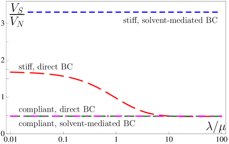
Figure 3: Swimming speed normalized by Newtonian swimming speed, $V_{s}/V_{N}$, as a function of incompressibility, $\lambda/\mu$. Compressibility effects can enhance swimming speeds for direct network-sheet BC. Swimming speed is enhanced relative to the Newtonian case for stiff networks or low frequencies (small $\eta\omega/\mu$). Red and green curves are for direct network-sheet BC and $\Xi=0$; blue and magenta curves are for solvent-mediated network-sheet BC. Red (long dashes): $\eta\omega/\mu=0.01$, $\Gamma/(\eta k^{2})=10$. Green (medium dashes): $\eta\omega/\mu=10$, $\Gamma/(\eta k^{2})=10$. Blue (short dashes): $\eta\omega/\mu=0.01$, $\Gamma/(\eta k^{2})=10$. Magenta (dash-dots): $\eta\omega/\mu=10$, $\Gamma/(\eta k^{2})=10$.

Compressibility effects are a possible mechanism for swimming speed enhancement. Fig. 3 show the swimming speed as a function of Lamé coefficient $\lambda$, a measure of incompressibility (the bulk modulus of compression is $2\mu+\lambda$). For direct sheet-network BC, the strongest enhancement of swimming speed occurs for a material with large shear modulus ($\mu\rightarrow\infty$) but which is maximally compressible ($\lambda=0$), and for a network which slips freely past the swimming sheet ($\Xi=0$). Compressibility does not strongly affect the swimming speed for solvent-mediated sheet-network BC. Swimming speeds can be faster than in Newtonian fluids for stiff networks/low frequencies (small $\eta\omega/\mu$), but not for compliant networks/high frequencies (large $\eta\omega/\mu$), reflecting a broader distinction which we address next.

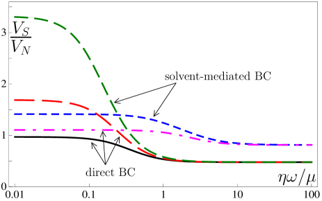
Figure 4: Swimming speed normalized by Newtonian swimming speed, $V_{s}/V_{N}$, as a function of $\eta\omega/\mu$. There is a transition at $\eta\omega/\mu\sim\eta k^{2}/\Gamma$ between fast swimming (stiff network/low frequencies, small $\eta\omega/\mu$) and slow swimming (compliant network/high frequences, large $\eta\omega/\mu$). Black, red and magenta curves are for direct network-sheet BC and $\Xi=0$; blue and green curves are for solvent-mediated network-sheet BC. Black (solid): $\lambda=\mu$, $\Gamma/(\eta k^{2})=10$. Red (long dashes): $\lambda=0$, $\Gamma/(\eta k^{2})=10$. Magenta (dash-dots): $\lambda=0$, $\Gamma/(\eta k^{2})=1$. Green (medium dashes): $\lambda=0$, $\Gamma/(\eta k^{2})=10$. Blue (short dashes): $\lambda=0$, $\Gamma/(\eta k^{2})=1$.

Fig. 4 plots the swimming velocity as a function of $\eta\omega/\mu$. There is a transition between two regimes, one for flexible networks or high frequency beating (small $\eta\omega/\mu$), leading to a smaller swimming velocity; and one for rigid networks or low frequency beating (large $\eta\omega/\mu$), leading to larger swimming velocities. The swimming speed enhancement is larger for larger values of $\Gamma$, and is larger for solvent-mediated network-sheet BC than for direct network-sheet BC. Physically, the transition between the two regimes corresponds to whether the network does not deform (stiff network/low frequencies) or whether the network deforms to move together with the solvent (compliant network/high frequencies). Since the network deforms due to drag forces from the solvent, one can predict that the transition between the two regimes occurs when the force/volume due to drag forces, $\sim\omega u\Gamma$, becomes comparable to the force/volume due to elasticity, $\sim\mu uk^{2}$, i.e. when $\eta\omega/\mu\sim\eta k^{2}/\Gamma$, which can be confirmed by comparing the curves in Fig. 4.

We can compare our results to those for the single-phase Brinkmann fluid [19, 17], which obeys $\eta\nabla^{2}\mathbf{v}-\nabla p=\Gamma^{B}\mathbf{v}$ and has swimming speed $V_{B}=V_{N}\sqrt{1+\Gamma^{B}/(\eta k^{2})}$. In the Brinkmann fluid the elastic phase is not a dynamic degree of freedom, but instead enters as an inert background retarding solvent motion. One expects that the two-fluid model behaves like a Brinkmann fluid when the network does not deform (i.e., $\eta\omega/\mu\ll\eta k^{2}/\Gamma$) and if $\Gamma^{B}=\Gamma$. This expectation is borne out in Fig. 5, but only for solvent-mediated BC. When the network deforms (compliant networks/high frequencies) the network-sheet BC do not greatly affect the swimming speed (magenta and green curves).

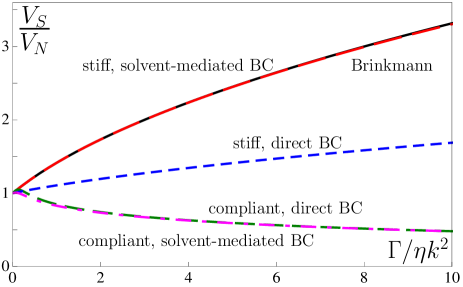
Figure 5: Swimming speed normalized by Newtonian swimming speed, $V_{s}/V_{N}$, as a function of drag coupling $\Gamma/\eta k$. The swimming speed is the same as in a Brinkmann fluid (black solid curve) for solvent-mediated network-sheet BC when the network does not deform (small $\eta\omega/\mu$). Blue and magenta curves are for direct network-sheet BC, $\Xi=0$, and $\lambda=0$; red and green curves are for solvent-mediated network-sheet BC and $\lambda=0$. Red (long dashes): $\eta\omega/\mu=0.01$. Green (medium dashes): $\eta\omega/\mu=10$. Blue (short dashes): $\eta\omega/\mu=0.01$. Magenta (dash-dots): $\eta\omega/\mu=10$.

Our results highlight the importance of understanding the proper boundary conditions for swimmers in gels. The boundary conditions need not be the same for all swimmers; they may depend on factors including swimmer morphology, surface biochemistry, or gel structure. However, one way to estimate whether a swimmer has direct interaction with the polymer network in a gel is to compare the swimmer size with the mesh size of the network. For example, sperm swimming in cervical mucus have head sizes of 3-5 $\mu$m. The mesh size of the network of mucin fibers in cervical mucus varies strongly with time during the menstrual cycle, with mesh sizes of up to 25 $\mu$m around ovulation, and as small as 200 nm at other times [25, 26]. Thus, during ovulation, when the sperm may be able to swim through the mucus while rarely encountering mucin fibers, solvent-mediated network-sheet BC likely apply. When the mesh sizes are small, direct network-sheet BC are more appropriate. Therefore, both types of boundary conditions described in this work may be relevant in biological situations. One important lesson is that even for an effective medium model of a heterogeneous material (such as our two-fluid model), microscopic heterogeneity will have strong consequences for the boundary conditions and corresponding swimming properties, since different boundary conditions lead to nearly 100% changes in swimming speeds in the stiff network limit.

Note that for the particular case of sperm in cervical mucus, the sperm are likely to be in the compliant network/high frequency phase: for well-hydrated mucus (near ovulation) when the mesh size is $\approx 10\;\mu$m, the shear modulus is $\approx 1$ Pa, and viscosity is $\approx 0.4$ Pa s; while farther from ovulation with mesh size $\approx 0.5\;\mu$m, the shear modulus is $\approx 4$ Pa and viscosity is $\approx 20$ Pa s [27]. Estimating $\Gamma\approx\eta/\xi^{2}$, where $\xi$ is the mesh size, and using a wavelength of sperm flagellar beating ($\approx 10\;\mu$m) to determine $k$, we estimate that near ovulation $\eta\omega/\mu\approx 10$ and $\Gamma/(\eta k^{2})\approx 0.03$, while away from ovulation $\eta\omega/\mu\approx 100$ and $\Gamma/(\eta k^{2})\approx 10$. Although for sperm the swimming speed enhancement seen in the stiff network/low frequency regime is unlikely to be realized in cervical mucus, for other swimmers in gels it may still be an important effect.

As we were completing this letter, we learned of the work of H. Wada [28], who has independently studied a closely related problem.

We are grateful to Charles Wolgemuth for many insightful conversations. This work was supported in part by National Science Foundation Grants Nos. CMMI-0825185 (VBS), DMS-0615919 (TRP), CBET-0854108 (TRP). HF and TRP thank the Aspen Center for Physics, where some of this work was done. We are grateful to H. Wada for sharing his work with us before it was published.

References

- [1] \NameLauga E. Powers T. R. \REVIEWRep. Prog. Phys. 722009096601.
- [2] \NameCelli J. P., Turner B. S., Afdhal N. H., Keates S., Ghiran I., Kelly C. P., Ewoldt R. H., McKinley G. H., So P., Erramilli S. Bansil R. \REVIEWProc. Natl. Acad. Sci. (USA) 106200914321.
- [3] \NameFauci L. J. Dillon R. \REVIEWAnnu. Rev. Fluid Mech. 382006371.
- [4] \NameSuarez S. S. Pacey A. A. \REVIEWHuman Reproduction Update 12200623.
- [5] \NameCanole-Parola E. \REVIEWAnn. Rev. Microbiol. 32197869.
- [6] \NameChaudhury T. K. \REVIEWJ. Fluid Mech. 951979189.
- [7] \NameFulford G. R., Katz D. F. Powell R. L. \REVIEWBiorheology 351998295.
- [8] \NameLauga E. \REVIEWPhys. Fluids 192007083104.
- [9] \NameFu H. C., Powers T. R. Wolgemuth C. W. \REVIEWPhys. Rev. Lett. 992007258101.
- [10] \NameFu H. C., Wolgemuth C. W. Powers T. R. \REVIEWPhys. Rev. E 782008041913.
- [11] \NameFu H. C., Wolgemuth C. W. Powers T. R. \REVIEWPhys. Fluids 212009033102.
- [12] \NameNormand T. Lauga E. \REVIEWPhys. Rev. E 782008061907.
- [13] \NameLauga E. \REVIEWEurophys. Lett. 86200964001.
- [14] \NameTeran J., Fauci L. Shelley M. \REVIEWPhys. Rev. Lett. 1042010038101.
- [15] \NameBerg H. C. Turner L. \REVIEWNature 2781979349.
- [16] \NameMagariyama Y. Kudo S. \REVIEWBiophys. J. 832002733.
- [17] \NameLeshansky A. M. \REVIEWPhys. Rev. E 802009051911.
- [18] \NameHappel J. Brenner H. \BookLow Reynolds number hydrodynamics (Prentice-Hall, Englewood Cliffs, NJ) 1965.
- [19] \NameSiddiqui A. M. Ansari A. R. \REVIEWJ. Porous Media 62003235.
- [20] \NameTaylor G. I. \REVIEWProc. R. Soc. Lond. Ser. A 2091951447.
- [21] \NameLevine A. J. Lubensky T. C. \REVIEWPhys. Rev. E 632001041510.
- [22] \Namede Gennes P. G. \REVIEWMacromolecules 91976587.
- [23] \NameMilner S. T. \REVIEWPhys. Rev. E 4819933674.
- [24] \NameFu H. C., Shenoy V. B. Powers T. R. \REVIEWPhys. Rev. E 782008061503.
- [25] \NameRuttlant J., López-Béjar M. López-Gatius F. \REVIEWAnat. Histol. Embryol. 40200579 .
- [26] \NameRuttlant J., López-Béjar M., Camón J., Martí M. López-Gatius F. \REVIEWAnat. Histol. Embryol. 302001159.
- [27] \NameTam P. Y., Katz D. F. Berger S. A. \REVIEWBiorheol. 171980465.
- [28] \NameWada H. \REVIEWPumping viscoelastic two-fluid media 2010.