A simple model of a vesicle drop in a confined geometry

Abstract

We present the exact solution of a two-dimensional directed walk model of a drop, or half vesicle, confined between two walls, and attached to one wall. This model is also a generalisation of a polymer model of steric stabilisation recently investigated. We explore the competition between a sticky potential on the two walls and the effect of a pressure-like term in the system. We show that a negative pressure ensures the drop/polymer is unaffected by confinement when the walls are a macroscopic distance apart.

1 Introduction

The study of the behaviour of the boundary between two phases has a long history [1, 2]. In two-dimensions where the boundary is one-dimensional much work has been done to understand such behaviour [3]. One type of model that has proved useful involves directed walks in a half plane with a Boltzmann weight associated with the area under the walk [4]. Related to this is the study of an enclosed boundary that can be used to model biological membranes [5]. The study of lattice vesicles is motivated by biological membranes that consist of lipid bi-layers and form shapes that depend on acidity, osmotic pressure and temperature. The basic model in two dimensions consists of some type of self-avoiding polygon on a lattice which is weighted according to its area and perimeter. The weighting of the area is analogous to an osmotic pressure. Various exactly solved cases including directed walk model have been considered [6, 7, 8].

In a parallel development the study of the behaviour of a long linear polymer molecule in dilute solution confined between two parallel plates [9] has recently gained momentum with the exact solution of various directed walk models [10, 11]. The phenomena being modelled here are the steric stabilisation and sensitised flocculation of colloidal dispersions. The progress made by the exact solution is the finding that if one considers a polymer confined between two sticky walls, the thermodynamic limit where the polymer is much longer than the distance between the walls is shown to have a different phase structure to the case where is there is one wall only [10].

In this paper we study a directed version of the self-avoiding vesicle model that is a generalisation of both the vesicle models studied previously [8] and the recently studied polymer model [10]. It is effectively a half-vesicle, or drop, if considered as a phase boundary. We consider directed self-avoiding walks on the square lattice, confined between two lines ($y=0$ and $y=w$) whose ends are both attached to one of the lines so that it effectively forms a polygon or rather a loop. We add weights for visits of the walk to both the top wall and the bottom wall. We also add an (osmotic) pressure-like term that weights the area contained under the loop.

Here we solve this model to show that introduction of such a negative (osmotic) pressure ensures that the two wall scenario behaves in the same way as the one wall case, in contrast to the model without any osmotic pressure.

2 The model

The directed walk model that we consider is closely related to Dyck paths. Dyck paths are directed walks on $\mathbb{Z}^{2}$ starting at $(0,0)$ and ending on the line $y=0$, which have no vertices with negative $y$-coordinates, and which have steps in the $(1,1)$ and $(1,-1)$ directions. We impose the additional geometrical constraint that the paths lie in the slit of width $w$ defined by the lines $y=0$ and $y=w$. We refer to Dyck paths that satisfy this slit constraint as loops (see figure 1).

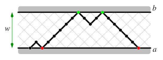
Figure 1: An example of a directed path which is a loop: both ends of the walk are fixed to be on the bottom wall.

Let $\mathcal{L}_{w}$ be the set of loops in the slit of width $w$. We define the generating function of these paths as follows:

$$L_{w}(z,a,b,p)=\sum_{\pi\in\mathcal{L}_{w}}z^{n(\pi)}a^{u(\pi)}b^{v(\pi)}p^{m(\pi)};$$ (2.1)

where $n(\pi),u(\pi)$, $v(\pi)$ and $m(\pi)$ are the number of edges in the path $\pi$, the number of vertices in the line $y=0$ (excluding the zeroth vertex), the number of vertices in the line $y=w$, and the area under the walk counted as the number of half-faces of the lattice between the walk and the line $y=0$, respectively.

Let $\mathcal{L}_{w}^{n}$ be the sets of loops of fixed length $n$ in the slit of width $w$. The partition function of loops is defined as

$$Z_{n}(w;a,b,q)=\sum_{\pi\in\mathcal{L}_{w}^{n}}a^{u(\pi)}b^{v(\pi)}q^{m(\pi)}\;.$$ (2.2)

Hence the generating function is related to the partition functions in the standard way, and for loops we have

$$L_{w}(z,a,b,p)=\sum_{n=0}^{\infty}z^{n}Z_{n}(w;a,b,p).$$ (2.3)

We define the reduced free energy $\kappa(w;a,b,q)$ for loops for fixed finite $w$ as

$$\kappa(w;a,b,p)=\lim_{n\rightarrow\infty}n^{-1}\log Z_{n}(w;a,b,p)\;.$$ (2.4)

Consider the singularities $z_{c}(w;a,b,p)$ of the generating functions $L_{w}(z,a,b,p)$ closest to the origin and on the positive real axis, known as the critical points. Given that the radii of convergence of the generating functions are finite, which we shall demonstrate, and since the partition functions are positive, by Pringsheim’s Theorem (see e.g. Theorem IV.6 in [12]) the critical points exist and are equal in value to the radii of convergence. Hence the free energies exist and one can relate the critical points to the reduced free energies as

$$\kappa(w;a,b,p)=-\log z_{c}(w;a,b,p).$$ (2.5)

3 The half-plane

3.1 Preliminaries

We first consider the case in which $w\to\infty$, which reduces the problem to the adsorption of paths to a wall in the half-plane with osmotic pressure.

We begin by noting that once $w>n$ for any finite length walk there can no longer be any visits to the top surface so

$$\mathcal{L}_{w+1}^{n}=\mathcal{L}_{w}^{n}\qquad\mbox{for $w>n$.}$$ (3.1)

Hence we define the sets $\mathcal{L}_{hp}^{n}$ as

$$\mathcal{L}_{hp}^{n}=\mathcal{L}_{n+1}^{n}\;.$$ (3.2)

The limit $w\to\infty$ can therefore be taken explicitly.

Also, as a consequence of the above, for all $w>n$ we have $v(\pi)=0$ for any $\pi\in\mathcal{L}_{w}^{n}$. Hence the partition function of loops in the half-plane can be defined as

$$Z_{n}^{hp}(a,p)=\sum_{\pi\in\mathcal{L}_{hp}^{n}}a^{u(\pi)}p^{m(\pi)}\;.$$ (3.3)

We define the generating function of loops in the half plane via the partition function as

$$L^{hp}(z,a,p)=\sum_{n=0}^{\infty}z^{n}Z_{n}^{hp}(a,p)\;.$$ (3.4)

In an analogous way to the slit we define the reduced free energy in the half-plane for loops as

$$\kappa^{hp}(a,p)=\lim_{n\rightarrow\infty}n^{-1}\log Z_{n}^{hp}(a,p)=-\log z^{hp}_{c}(a,p).$$ (3.5)

We note that in defining these free energies for the half-plane the thermodynamic limit $n\rightarrow\infty$ is taken after the limit $w\to\infty$: we shall return to this order of limits later.

3.2 Exact solution for the generating function in the half-plane

We use a standard decomposition argument to derive a functional equation for the generating function $L^{hp}(z,a,p)$ as follows. Except for the zero-step Dyck path with weight $1$, every Dyck path can be decomposed uniquely into a Dyck path bracketed by a pair of up and down steps, followed by another Dyck path. The associated generating functions are $apz^{2}L^{hp}(pz,1,p)$ and $L^{hp}(z,a,p)$, respectively. This decomposition leads to the functional equation

$$L^{hp}(z,a,p)=1+apz^{2}L^{hp}(pz,1,p)L^{hp}(z,a,p)\;,$$ (3.6)

which one can rewrite as

$$L^{hp}(z,a,p)=\frac{1}{1-apz^{2}L^{hp}(pz,1,p)}\;.$$ (3.7)

By iterating this equation one can find a continued fraction expansion for $L^{hp}(z,a,p)$ as

$$L^{hp}(z,a,p)=\cfrac{1}{1-\cfrac{apz^{2}}{1-\cfrac{p^{3}z^{2}}{1-\cfrac{p^{5}z^{2}}{1-\cfrac{p^{7}z^{2}}{1-\ldots}}}}}\;.$$ (3.8)

One can find this solution in the literature [14]. To find a series solution one can use a linearisation Ansatz, standard for a $q$-deformed algebraic equation such as Equation (3.6). We substitute

$$L^{hp}(z,1,p)=\frac{H(pz,p)}{H(z,p)}$$ (3.9)

into Equation (3.6) with $a=1$, and find that $H(z,q)$ must satisfy the linear $q$-functional equation

$$H(pz,p)-H(z,p)-pz^{2}H(p^{2}z,p)=0\;.$$ (3.10)

We then solve this linear functional equation using a series in $z$,

$$H(z,p)=\sum_{n=0}^{\infty}c_{n}(p)z^{n}\;.$$ (3.11)

This leads to the simple two-term recurrence

$$(1-p^{n})c_{n}-p^{2n-3}c_{n-2}=0\;.$$ (3.12)

By iteration and using initial conditions $c_{0}=1$ and $c_{1}=0$ one finds

$$H(z,p)=\sum_{m=0}^{\infty}\frac{p^{2m(m-1)}}{(p^{2};p^{2})_{m}}(-pz^{2})^{m}\;.$$ (3.13)

Here $(t;q)_{n}=\prod_{k=0}^{n-1}(1-tq^{k})$ is the standard $q$-product. Using basic hypergeometric series notation [13], we identify $H(z,p)={}_{0}\phi_{1}(-;0;p^{2},-pz^{2})$, where ${}_{0}\phi_{1}(-;b;q,t)$ is given by

$${}_{0}\phi_{1}(-;b;q,t)=\sum_{n=0}^{\infty}\frac{q^{n^{2}-n}}{(b;q)_{n}(q;q)_{n}}t^{n}\;.$$ (3.14)

Via (3.7) and (3.9) we arrive at the final result

$$L^{hp}(z,a,p) =\frac{H(pz,p)}{H(pz,p)-apz^{2}H(p^{2}z,p)}$$

$$=\frac{H(pz,p)}{aH(z,p)+(1-a)H(pz,p)}\;,$$ (3.15)

where $H(z,p)={}_{0}\phi_{1}(-;0;p^{2},-pz^{2})$.

4 Exact solution for the generating functions in finite width strips

The solution of the strip problem begins by using an argument that builds up configurations (uniquely) in a strip of width $w+1$ from configurations in a strip of width $w$. In this way a recurrence-functional equation is constructed. Consider configurations of loops in a strip of width $w$ (see figure 2), and focus on the vertices touching the top wall: call these top vertices. These vertices contribute a factor $b$ to the Boltzmann weight of the configuration. Now consider a zig-zag path (see figure 2), which is defined as a path of any even length, or one of length zero, in a strip of width 1. The generating function of zig-zag paths is $1/(1-bpz^{2})$. Replace each of the top vertices in the configuration by any zig-zag path. Since one could choose a single vertex as the zig-zag path all configurations that fit in a strip of width $w$ are reproduced. Also, the addition of any non-zero length path at any top vertex will result in a new configuration of width $w+1$ and no more. The inverse process is also well defined and so we can write recurrence-functional equations for each of the generating functions.

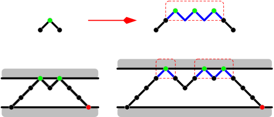
Figure 2: The construction of configurations in strip width $w+1$ from configurations in strip width $w$ is illustrated. Every vertex touching the upper wall in the strip of width $w$ can be replaced by a zig-zag path as shown.

The generating function $L_{w}(z,a,b,p)$ satisfies the following functional recurrence:

$$L_{1}(z,a,b,p) = \frac{1}{1-abpz^{2}};$$ (4.1)

$$L_{w}(z,a,b,p) = L_{w-1}\left(z,a,\frac{1}{1-bp^{2w-1}z^{2}},p\right).$$ (4.2)

We note that the zeroth vertex of the path is weighted $1$ and that $L_{w}(z,a,b,p)$ counts the walk consisting of a single vertex. We see that

$$L_{2}(z,a,b,p)=\cfrac{1}{1-\cfrac{apz^{2}}{1-bp^{3}z^{2}}}$$ (4.3)

and

$$L_{3}(z,a,b,p)=\cfrac{1}{1-\cfrac{apz^{2}}{1-\cfrac{p^{3}z^{2}}{1-bp^{5}z^{2}}}}\;.$$ (4.4)

Hence, by substitution, this functional recurrence generates a finite continued fraction expansion of the generating function

$$L_{w}(z,a,b,p)=\cfrac{1}{1-\cfrac{apz^{2}}{1-\cfrac{p^{3}z^{2}}{1-\cfrac{p^{5}z^{2}}{1-\cfrac{p^{7}z^{2}}{\genfrac{}{}{0.0pt}{}{}{\ddots\genfrac{}{}{0.0pt}{}{}{\genfrac{}{}{0.0pt}{}{}{\genfrac{}{}{0.0pt}{}{}{\genfrac{}{}{0.0pt}{}{}{\cfrac{p^{2w-3}z^{2}}{1-bp^{2w-1}z^{2}}}}}}}}}}}}\;.$$ (4.5)

This finite continued fraction can be compared directly to (3.8), which is formally obtained by taking the limit of $w\to\infty$. Conversely, $L_{w}(z,a,b,p)$ is a finitary version of $L^{hp}(z,a,p)$.

It is clear that the generating function can also be written as a rational function

$$L_{w}(z,a,b,p)=\frac{P_{w}(z,a,b,p)}{Q_{w}(z,a,b,p)}$$ (4.6)

though it does not simply follow to write expressions for these. It does however follow from the theories of continued fractions and orthogonal polynomials (see pages 256–257 of Andrews, Askey and Roy [15]) that both the numerator $P_{w}$ and denominator $Q_{w}$ of the generating function satisfy recursions

$$P_{w}(z,a,b,p)=\begin{cases}1\;,&w=1\\ 1-bp^{3}z^{2}\;,&w=2\\ P_{w-1}(z,a,1,p)-bp^{2w-1}z^{2}P_{w-2}(z,a,1,p)\;&w\geq 3\;,\end{cases}$$ (4.7)

and

$$Q_{w}(z,a,b,p)=\begin{cases}1-abpz^{2}\;,&w=1\\ 1-apz^{2}-bp^{3}z^{2}\;,&w=2\\ Q_{w-1}(z,a,1,p)-bp^{2w-1}z^{2}Q_{w-2}(z,a,1,p)\;,&w\geq 3\;.\end{cases}$$ (4.8)

One can immediately note that

$$P_{w}(z,a,b,p)=Q_{w}(z,0,b,p)$$ (4.9)

so that

$$L_{w}(z,a,b,p)=\frac{Q_{w}(z,0,b,p)}{Q_{w}(z,a,b,p)}\;.$$ (4.10)

We now form the width generating function for the denominator as

$$W(t,z,a,b,p)=\sum_{w=0}^{\infty}Q_{w}(z,a,b,p)t^{w}\;,$$ (4.11)

and find a functional equation for $W(t)$ from the recurrence (4.8) as

$$W(t,z,a,b,p)=\\ t(1-t)(1-abpz^{2})+t^{2}(1-apz^{2}-bp^{3}z^{2})+tW(t,z,a,1,p)-bp^{3}z^{2}t^{2}W(p^{2}t,z,a,1,p)\;.$$ (4.12)

One can first solve for $W(t,z,a,1,p)$ by iteration to give

$$W(t,z,a,1,p)=\\ \sum_{n=0}^{\infty}\frac{(-1)^{n}p^{2n^{2}+2n}z^{n}t^{2n}\left[tp^{2n}(1-tp^{2n})(1-apz^{2})+t^{2}p^{4n}(1-apz^{2}-p^{3}z^{2})\right]}{(t;p^{2})_{n+1}}$$ (4.13)

It is then straightforward to provide an expression for $W(t,z,a,b,p)$ by substituting into the functional equation (4.12). To simplify the expressions further, let us rewrite our expression for $W(t,z,a,1,p)$ in terms of

$$\phi(t,q,x)=\sum_{n=0}^{\infty}\frac{q^{n(n-1)}x^{n}}{(t,q)_{n}}\;.$$ (4.14)

Using basic hypergeometric series notation [13], we identify $\phi(t,q,x)={}_{1}\phi_{2}(q;0,t;q,x)$. With help of $\phi(t,q,x)$ we can write

$$W(t,z,a,1,p)=\frac{1-apz^{2}}{pz^{2}t}-1-\frac{1-apz^{2}}{pz^{2}t}\phi(t,p^{2},-pz^{2}t^{2})+\phi(t,p^{2},-p^{3}z^{2}t^{2})\;,$$ (4.15)

which leads to

$$W(t,z,a,b,p)=\frac{b+t-bt-apz^{2}t-bpz^{2}t-ap^{2}z^{4}t^{3}+abpz^{2}t+abp^{2}z^{4}t^{3}-abpz^{2}}{pz^{2}t}\\ +\frac{(bt-b-t)(1-apz^{2})}{pz^{2}t}\phi(t,p^{2},-pz^{2}t^{2})-(bt-b-t)\phi(t,p^{2},-p^{3}z^{2}t^{2})\;.$$ (4.16)

To obtain an explicit expression for $Q_{w}$ one first expands the $q$-product in the function $\phi$ with the help of the $q$-binomial theorem [13] to obtain

$$\phi(t,q,xt^{2})=1+\sum_{m=0}^{\infty}t^{m}\sum_{n=1}^{\infty}q^{n(n-1)}\genfrac{[}{]}{0.0pt}{}{m-n-1}{n-1}_{q}x^{n}\;,$$ (4.17)

where the $q$-binomial coefficient is defined as

$$\genfrac{[}{]}{0.0pt}{}{N}{M}_{q}=\begin{cases}\dfrac{(q;q)_{N}}{(q;q)_{M}(q;q)_{N-M}}&0\leq M\leq N\;,\\ 0&\text{otherwise.}\end{cases}$$ (4.18)

After some algebraic manipulations this gives us an explicit and surprisingly elegant expression for $Q_{w}$ as

$$Q_{w}(z,a,b,p)=\sum_{m=0}^{\infty}(-pz^{2})^{m}p^{2m(m-1)}\times\\ \left((1-b)\genfrac{[}{]}{0.0pt}{}{w-m}{m}_{p^{2}}+b\genfrac{[}{]}{0.0pt}{}{w-m+1}{m}_{p^{2}}-(1-a)(1-b)\genfrac{[}{]}{0.0pt}{}{w-m+1}{m-1}_{p^{2}}-(1-a)b\genfrac{[}{]}{0.0pt}{}{w-m}{m-1}_{p^{2}}\right)\;,$$ (4.19)

and hence via (4.10) an explicit expression for the generation function for loops $L_{w}$,

$$L_{w}(z,a,b,p)=\\ \frac{\sum\limits_{m=0}^{\infty}(-pz^{2})^{m}p^{2m(m-1)}\left((1-b)\genfrac{[}{]}{0.0pt}{}{w-m}{m}_{p^{2}}+b\genfrac{[}{]}{0.0pt}{}{w-m+1}{m}_{p^{2}}-(1-b)\genfrac{[}{]}{0.0pt}{}{w-m+1}{m-1}_{p^{2}}-b\genfrac{[}{]}{0.0pt}{}{w-m}{m-1}_{p^{2}}\right)}{\sum\limits_{m=0}^{\infty}(-pz^{2})^{m}p^{2m(m-1)}\left((1-b)\genfrac{[}{]}{0.0pt}{}{w-m}{m}_{p^{2}}+b\genfrac{[}{]}{0.0pt}{}{w-m+1}{m}_{p^{2}}-(1-a)(1-b)\genfrac{[}{]}{0.0pt}{}{w-m+1}{m-1}_{p^{2}}-(1-a)b\genfrac{[}{]}{0.0pt}{}{w-m}{m-1}_{p^{2}}\right)}\;.$$ (4.20)

Note that the sums involved only have finitely many non-zero terms, as the $q$-binomial coefficients are zero when $m>\lfloor w/2+1\rfloor$.

For $a=b=1$ we obtain the particularly simple identity

$$L_{w}(z,1,1,p)=1-\frac{\sum\limits_{m=0}^{\infty}(-pz^{2})^{m}p^{2m(m-1)}\genfrac{[}{]}{0.0pt}{}{w-m}{m-1}_{p^{2}}}{\sum\limits_{m=0}^{\infty}(-pz^{2})^{m}p^{2m(m-1)}\genfrac{[}{]}{0.0pt}{}{w-m+1}{m}_{p^{2}}}\;.$$ (4.21)

5 Analysis of the free energy

5.1 Finite width

When the width is finite ($w<\infty$) the system is effectively one-dimensional and so there cannot be any phase transitions at finite temperatures. Mathematically, one can see this in the following way. Regardless of whether $p=1$ or $p<1$ the generating function $L_{w}(z,a,b,p)$ is a ratio of polynomials $P_{w}(z,a,b,p)$ and $Q_{w}(z,a,b,p)$. As such the only singularities in the generating function occur at zeros of $Q_{w}(z,a,b,p)$. Given that these are orthogonal polynomials satisfying the same three-term recurrence, albeit with different initial conditions, the zeros of $P_{w}(z,a,b,p)$ are distinct to those of $Q_{w}(z,a,b,p)$. The simple zero in $Q_{w}$ leads to a simple pole in $L_{w}$. The location of the zero $z_{c}(w;a,b,p)$ is an analytic function of $a$, $b$ and $p$.

5.2 Half-plane limit

We now use that

$$\lim_{w\rightarrow\infty}\genfrac{[}{]}{0.0pt}{}{w-m}{m}_{p^{2}}=\frac{1}{(p^{2},p^{2})_{m}}$$ (5.1)

to give

$$\lim_{w\rightarrow\infty}Q_{w}(z,a,b,p) =\sum_{m=0}^{\infty}(-pz^{2})^{m}p^{2m(m-1)}\left[\frac{1}{(p^{2},p^{2})_{m}}-(1-a)\frac{1}{(p^{2},p^{2})_{m-1}}\right]$$ (5.2)

$$=H(z,p)-(a-1)pz^{2}H(p^{2}z,p)$$

$$=aH(z,p)+(1-a)H(pz,p)$$

and

$$\lim_{w\rightarrow\infty}P_{w}(z,a,b,p) =\lim_{w\rightarrow\infty}Q_{w}(z,0,b,p)=H(pz,p)\;.$$ (5.3)

One can therefore demonstrate explicitly that for $p<1$

$$\lim_{w\rightarrow\infty}L_{w}(z,a,b,p)=L^{hp}(a,p)=\frac{H(pz,p)}{aH(z,p)+(1-a)H(pz,p)}\;.$$ (5.4)

The series $H(z,p)$ converges absolutely for any $z$ provided $p<1$, and so has no singularities as a function of $z$. Therefore, the only singularity of $L^{hp}(a,p)$ occurs as a result of zeros of $H(z,p)-(a-1)pz^{2}H(p^{2}z,p)$ provided they don’t cancel with zeros of the numerator. As such, consider that the denominator can be written as $H(pz,p)-apz^{2}H(p^{2}z,p)$ and that the numerator is $H(pz,p)$. For small $z$ we have that $H(z,p)$ is positive since $H(0,p)=1$. Consider the smallest positive zero of the $H(pz,p)$: let us call it $z_{p}$. Now since $p<1$ we have $H(p^{2}z_{p},p)>0$ so that the first zero of $H(pz,p)-apz^{2}H(p^{2}z,p)$ must occur at some value $z_{c}<z_{p}$: that is, no cancellation occurs.

Necessarily the closely singularity to the origin of $L^{hp}(a,p)$ is then an analytic function of $a$. Hence there is no phase transition as a function of $a$.

The situation for $p=1$ is different and well-known. It has been shown [10] previously that

$$\lim_{w\rightarrow\infty}L_{w}(z,a,b,1)=L^{hp}(a,1)=\frac{1+\sqrt{1-4z^{2}}}{1+\sqrt{1-4z^{2}}-2az^{2}}\;.$$ (5.5)

Considered as power series in $z$, the denominator (and numerator) of the half-plane generating function only converges for $z<1/2$. For small $a$ the algebraic singularity at $z=1/2$ is the closest to the origin while for $a>2$ the pole arising from the zero in the denominator is closer. This leads to a phase transition on varying $a$.

5.3 Infinite slit limit

Let us consider the limit for $p<1$ of

$$\lim_{w\rightarrow\infty}z_{c}(w;a,b,p)\;.$$ (5.6)

As we have discussed above $z_{c}(w;a,b,p)$ arises from a zero of the polynomial $Q_{w}(z,a,b,p)$ while $z_{c}^{hp}(a,p)$ arises from a zero of $H(z,p)-(a-1)pz^{2}H(p^{2}z,p)$ which is analytic for all $z$. Now we have that the limit of $Q_{w}(z,a,b,p)$ is the half plane denominator $H(z,p)-(a-1)pz^{2}H(p^{2}z,p)$ for all $z$. Hence, since the zero at $z_{c}^{hp}(a,p)$ does not cancel with a zero in the numerator as shown above we can deduce

$$\lim_{w\rightarrow\infty}z_{c}(w;a,b,p)=z_{c}^{hp}(a,p)\;.$$ (5.7)

We also know that $z_{c}(w;a,b,p)$ is an analytic function of $a$ and $b$ for any fixed $w$ and $p$ and that $z_{c}^{hp}(a,p)$ is also analytic in $a$.

Importantly, the argument fails when $p=1$ because the limit of the denominators for finite widths have a factor, depending on $b$, that does cancel with one in the numerator.

6 Comparison of $p<1$ with $p=1$ cases

To summarise for $p<1$ we have just argued that the free energy of our model is the same in the infinite slit and the half plane scenarios:

$$\kappa^{inf-slit}(a,b,p)\equiv\lim_{w\rightarrow\infty}\kappa(w;a,b,p)=\kappa^{hp}(a,p)$$ (6.1)

for all $a$, $b$ and that $\kappa^{hp}(a,p)$ is an analytic function of $a$. On the other hand we know [10] that for $p=1$

$$\kappa^{inf-slit}(a,b,1)\equiv\lim_{w\rightarrow\infty}\kappa(w;a,b,1)=\left\{\begin{array}[]{ll}\log(2)&\mbox{ if }a,b\leq 2\\ \log\left(\frac{a}{\sqrt{a-1}}\right)&\mbox{ if }a>2\mbox{ and }a>b\\ \log\left(\frac{b}{\sqrt{b-1}}\right)&\mbox{ otherwise.}\end{array}\right.$$ (6.2)

while that

$$\kappa^{hp}(a,1)=\left\{\begin{array}[]{cc}\log(2)&a\leq 2\\ \log\left(\frac{a}{\sqrt{a-1}}\right)&a>2.\end{array}\right.$$ (6.3)

Hence for $b>\max(a,2)$

$$\kappa^{inf-slit}(a,b,1)\neq\kappa^{hp}(a,1)$$ (6.4)

and so the two-wall infinite slit scenario is physically different to the one wall half-plane for $p=1$.

From a physical point of view the $p=1$ case is more complicated than the $p<1$ cases in that there are phase transitions in both the half-plane and infinite slit scenarios and, crucially, these are not all coincident. For $p<1$ the infinite slit and the half-plane are the same. This implies that for $p<1$ (negative pressure) in the infinite slit the top wall plays no part physically in the behaviour of the system. For $p=1$, while the walls are a macroscopic distance apart in the infinite slit, the polymer can still feel both walls, recalling that the polymer is also macroscopic in length.

We have solved a simple model of a vesicle confined in a slit. Mathematically the solution is interesting as it provides a new orthogonal polynomial series associated with Dyck paths. Physically it demonstrates that an osmotic pressure term can remove the effect of confinement and the effect of a contact potential with a far wall no matter how strong the potential. Interesting further work would be to investigate the scaling around the limit $w\rightarrow\infty$ and $p\rightarrow 1$.

References

• [1] H.Β N.Β V. Temperley, Proc. Camb. Phil. Soc. 48, 638 (1952).
• [2] S.Β Dietrich, in Phase Transitions and Critical Phenomena, edited by C.Β Domb and J.Β L. Lebowitz, volumeΒ 12, pageΒ 1, Academic, London, 1988.
• [3] M.Β E. Fisher, J. Stat. Phys. 34, 667 (1984).
• [4] A.Β L. Owczarek and T.Β Prellberg, J. Stat. Phys. 70, 1175 (1993).
• [5] M.Β E. Fisher, A.Β J. Guttmann, and S.Β Whittington, J. Phys. A 24, 3095 (1991).
• [6] R.Β Brak and A.Β J. Guttmann, J. Phys A. 23, 4581 (1990).
• [7] R.Β Brak, A.Β L. Owczarek, and T.Β Prellberg, J. Stat. Phys. 76, 1101 (1994).
• [8] T.Β Prellberg and A.Β L. Owczarek, J. Stat. Phys. 80, 755 (1995).
• [9] E.Β J. Janse van Rensburg, E.Β Orlandini, A.Β L. Owczarek, A.Β Rechnitzer, and S.Β Whittington, J. Phys. A 38, L823 (2005).
• [10] R.Β Brak, A.Β L. Owczarek, A.Β Rechnitzer, and S.Β Whittington, J. Phys. A 38, 4309 (2005).
• [11] A.Β L. Owczarek, R.Β Brak, and A.Β Rechnitzer, J. Math. Chem. 45, 113 (2008).
• [12] P.Β Flajolet and R.Β Sedgewick, Analytic Combinatorics, Cambridge University Press, Cambridge, 2009
• [13] G.Β Gasper and M.Β Rahman, volumeΒ 96 of Encyclopedia of Mathematics and its Applications, Cambridge University Press, Cambridge, 2004.
• [14] E.Β J. Janse van Rensburg, The Statistical Mechanics of Interacting Walks, Polygons, Animals and Vesicles, Oxford University Press, Oxford, 2000.
• [15] G.Β E. Andrews, R.Β Askey, and R.Β Roy, volumeΒ 71 of Encyclopedia of Mathematics and its Applications, Cambridge University Press, Cambridge, 1999.