Knudsen gas in a finite random tube: transport diffusion and first passage properties

Abstract

We consider transport diffusion in a stochastic billiard in a random tube which is elongated in the direction of the first coordinate (the tube axis). Inside the random tube, which is stationary and ergodic, non-interacting particles move straight with constant speed. Upon hitting the tube walls, they are reflected randomly, according to the cosine law: the density of the outgoing direction is proportional to the cosine of the angle between this direction and the normal vector. Steady state transport is studied by introducing an open tube segment as follows: We cut out a large finite segment of the tube with segment boundaries perpendicular to the tube axis. Particles which leave this piece through the segment boundaries disappear from the system. Through stationary injection of particles at one boundary of the segment a steady state with non-vanishing stationary particle current is maintained. We prove (i) that in the thermodynamic limit of an infinite open piece the coarse-grained density profile inside the segment is linear, and (ii) that the transport diffusion coefficient obtained from the ratio of stationary current and effective boundary density gradient equals the diffusion coefficient of a tagged particle in an infinite tube. Thus we prove Fick’s law and equality of transport diffusion and self-diffusion coefficients for quite generic rough (random) tubes. We also study some properties of the crossing time and compute the Milne extrapolation length in dependence on the shape of the random tube.
Keywords: cosine law, Knudsen random walk, random medium, self-diffusion coefficient, transport diffusion coefficient, random walk in random environment
AMS 2000 subject classifications: 60K37. Secondary: 37D50, 60J25

${}^{~{}1}$Université Paris 7, UFR de Mathématiques, case 7012, 2, place Jussieu, F–75251 Paris Cedex 05, France
e-mail: comets@math.jussieu.fr, url: http://www.proba.jussieu.fr/$\sim$comets

${}^{~{}2}$Department of Statistics, Institute of Mathematics, Statistics and Scientific Computation, University of Campinas–UNICAMP, rua Sérgio Buarque de Holanda 651, CEP 13083–859, Campinas SP, Brazil
e-mails: popov@ime.unicamp.br, marinav@ime.unicamp.br
urls: http://www.ime.unicamp.br/$\sim$popov, http://www.ime.unicamp.br/$\sim$marinav

${}^{~{}3}$Forschungszentrum Jülich GmbH, Institut für Festkörperforschung, D–52425 Jülich, Deutschland
e-mail: G.Schuetz@fz-juelich.de,
url: http://www.fz-juelich.de/iff/staff/Schuetz_G/

1 Introduction

Diffusion in stationary states may be encountered either in equilibrium, where no macroscopic mass or energy fluxes are present in a system of many diffusing particles, or away from equilibrium, where diffusion is often driven by a density gradient between two open segments of the surface that encloses the space in which particles diffuse. In equilibrium states, one is interested in the self-diffusion coefficient ${\mathsf{D}}_{\text{self}}$, as given by the mean-square displacement (MSD) of a tagged particle. This quantity, also called tracer diffusion coefficient, can be measured using e.g. neutron scattering, NMR or direct video imaging in the case of colloidal particles. In gradient-driven non-equilibrium steady states, there is a particle flux between the boundaries which is proportional to the density gradient. This factor of proportionality is the so-called transport or collective diffusion coefficient ${\mathsf{D}}_{\text{trans}}$.

Often these two diffusion coefficients cannot be measured simultaneously under concrete experimental conditions and the question arises whether one can infer knowledge about the other diffusion coefficient, given one of them. Generally, in dense systems these diffusion coefficients depend in a complicated fashion on the interaction between the diffusing particles. In the case of diffusion in microporous media, e.g. in zeolites, however, the mean free path of the particles is of the order of the pore diameter or even larger. Then diffusion is dominated by the interaction of particles with the pore walls rather than by direct interaction between particles. In this dilute so-called Knudsen regime neither ${\mathsf{D}}_{\text{self}}$ nor ${\mathsf{D}}_{\text{trans}}$ depend on the particle density anymore, but are just given by the low-density limits of these two quantities. One then expects ${\mathsf{D}}_{\text{self}}$ and ${\mathsf{D}}_{\text{trans}}$ to be equal. This assumption is a fundamental input into the interpretation of many experimental data, see e.g. [14] for an overview of diffusion in condensed matter systems.

Not long ago this basic tenet has been challenged by Monte-Carlo simulation of Knudsen diffusion in pores with fractal pore walls [16, 17, 18]. The authors of these (and further) studies concluded that self-diffusion depends on the surface roughness of a pore, while transport diffusion is independent of it. In other words, the authors of [16, 17, 18] argue that even in the low density limit, where the gas particle are independent of each other and interact only with the pore walls, ${\mathsf{D}}_{\text{self}}\neq{\mathsf{D}}_{\text{trans}}$, with a dependence of ${\mathsf{D}}_{\text{self}}$ on the details of the pore walls that ${\mathsf{D}}_{\text{trans}}$ does not exhibit. This counterintuitive numerical finding was quickly questioned on physical grounds and contradicted by further simulations [21] which give approximate equality of the two diffusion coefficients. These controversial results gave rise to a prolonged debate which finally led to the consensus that indeed both diffusion coefficients should agree for the Knudsen case [24]. It has remained open though whether these diffusion coefficients are generally exactly equal or only approximately to a degree depending on the details of the specific setting.

A physical argument put forward in [25] suggests general equality. To see this one imagines the following gedankenexperiment. Imagine one colours in a equilibrium setting of many non-interacting particles some of these particles without changing their properties. At some distance from this colouring region the colour is removed. Then these coloured particles experience a density gradient just as “normal” particles in an open system with the same pore walls would. Since the walls are essentially the same and the properties of coloured and uncoloured particles are the same, the statistical properties of the ensemble of trajectories remain unchanged. Hence one expects any pore roughness to have the same effect on diffusion, irrespective of whether one consider transport diffusion or self-diffusion. Notice, however, that this microscopic argument, while intuitively appealing, is far from rigorous. First, the precise conditions under which the independence of the diffusion coefficients on the pore surface is supposed to be valid, is not specified. This is more than a technical issue since one may easily construct surface properties leading to non-diffusive behaviour (cf. [7, 20]). Second, there is no obvious microscopic interpretation or unique microscopic definition of the transport diffusion coefficient for arbitrary surface structures. ${\mathsf{D}}_{\text{trans}}$ is a genuinely macroscopic quantity and a proof of equality between ${\mathsf{D}}_{\text{trans}}$ and ${\mathsf{D}}_{\text{self}}$ (which is naturally microscopically defined through the asymptotic long-time behaviour of the MSD) requires some further work and new ideas. One needs to establish that on large scales the Knudsen process converges to Brownian motion (which then also gives ${\mathsf{D}}_{\text{self}}$). Moreover, in order to compare ${\mathsf{D}}_{\text{trans}}$ and ${\mathsf{D}}_{\text{self}}$ one needs a precise macroscopic definition of ${\mathsf{D}}_{\text{trans}}$ which is independent of microscopic properties of the system.

The first part of this programme is carried out in [7]. There we proved the quenched invariance principle for the horizontal projection of the particle’s position using the method of considering the environment viewed from the particle. This method is useful in a number of models related to Markov processes in a random environment, cf. e.g. [11, 12, 19]. The aim of this paper is to solve the second problem of defining ${\mathsf{D}}_{\text{trans}}$ and proving equality with ${\mathsf{D}}_{\text{self}}$. As in [7] we consider a random tube to model pore roughness. In contrast to [7], we now have to consider tubes of finite extension along the tube contour and introduce open segments at the ends of the tube. Doing this rigorously then clarifies some of the salient assumptions underlying the equality of ${\mathsf{D}}_{\text{trans}}$ and ${\mathsf{D}}_{\text{self}}$. Naturally, since we are in the dilute gas limit, there is no dependence on the particle density in either of the two diffusion constants. This obvious point has not been controversial and will not be stressed below.

We note that we define ${\mathsf{D}}_{\text{trans}}$ through stationary transport in an open system since this is accessible experimentally as well as numerically in Monte Carlo simulation. Indeed, in the literature that gave rise to the controversy that we address here, this way of defining ${\mathsf{D}}_{\text{trans}}$ is used, albeit in a non-rigorous fashion. Sticking to this experimentally motivated setting we shall give below a precise definition that can be used to prove rigorously that under rather generic circumstances ${\mathsf{D}}_{\text{trans}}={\mathsf{D}}_{\text{self}}$, which means that both diffusion constants depend on the pore surface in the same way. As pointed out above, this equality is expected from independence of the particles and the invariance principle for the process and its time-reversed. However, we could not find a general result applying here, and moreover, as it turns out, the proof is not entirely trivial. There are some technical difficulties to overcome because the quenched invariance principle of Definition 2.2 below is not very “strong” (there is no uniformity assumption on the speed of convergence as a function of the initial conditions) and the jumps of the embedded discrete-time billiard are not uniformly bounded. Let us mention here that it is generally difficult to obtain stronger results in the above sense, since the corrector technique, generally used in the proof of quenched central limit theorems for reversible Markov processes in random environment, is still not sufficiently well understood.

To further illuminate the contents of our results we point out that in a bulk system the equality of the self-diffusion coefficient and the transport diffusion coefficient for the spread of equilibrium density fluctuations in an infinite system may be taken for granted in the case of particles that have no mutual interaction. Hence another way of stating the main conclusion of our work is the assertion that the transport diffusion coefficient as defined here in a stationary far-from-equilibrium setting coincides with the usual equilibrium transport diffusion coefficient.

We also address finite-size effects coming from the fact that we are dealing with diffusion in a finite, open geometry. This causes deviations from bulk results for first-passage-time properties if a tagged particle starts its motion close to one boundary. In particular, we compute the permeation time and the Milne extrapolation length that characterizes the survival time of a particle injected at a boundary.

As a final introductory remark, it is worth noting that the case of Knudsen gas with the cosine reflection law (which is the model considered in this paper) is particularly easy to analyse because the stationary state can be written in an explicit form, cf. Theorem 2.8. As explained below, this is related to the following facts: (i) there is no interaction between particles, (ii) for random billiard (i.e., a motion of only one particle in a closed domain) with the cosine reflection law the stationary measure is quite explicit, as shown in [6]. Similar questions are much more complicated when the explicit form of the stationary state is not known. This is the general situation for non-equilibrium steady states. We refer to e.g. the model of [2] (a chain of coupled oscillators) where one resorts to a bound on the entropy production.

This paper is organized in the following way. In Section 2.1 we define the infinite random tube, and then introduce the process we call random billiard. In Section 2.2, we then consider a gas of independent particles with absorption/injection in a finite piece of the random tube, and we formulate our results on the stationary measure for that gas and on the transport diffusion coefficient. In Section 2.3, we go on to formulate first passage time results that concern exit from and crossing of the finite tube by a tagged particle. The remaining part of the paper is devoted to the proof of our results. In Section 3 we mainly use the reversibility of the process to obtain several technical facts used later. In Section 4 we prove the result on the stationary measure of the Knudsen gas in the finite tube. Section 5.1 contains the proofs of the results related to the transport diffusion coefficient, and in Section 5.2 we prove the results related to the crossing of the finite tube.

2 General notations and main results

Naively the transport diffusion coefficient in tube direction $x$ may be defined through the diffusion equation for the probability density $\partial_{t}P(x,t)=\partial_{x}(D(x)\partial_{x}P(x,t))$, where a possible $x$-dependence may originate from a spatial inhomogeneity of the tube. Denote by $J$ the particle current in the system; assuming stationarity with a probability density $P^{*}(x)$ one has $J=D(x)\partial_{x}P^{*}(x)$. With fixed external densities $P^{+}$ at $x=L$ and $P^{-}$ at $x=0$ one finds by integration $J={\mathsf{D}}_{\text{trans}}\vartheta$ with density gradient $\vartheta=(P^{+}-P^{-})/L$ and ${\mathsf{D}}_{\text{trans}}^{-1}=1/L\int_{0}^{L}dxD^{-1}(x)$. By measuring the current and the boundary densities one can thus obtain the transport diffusion coefficient without having to determine the local quantity $D(x)$. This result, however, implies knowledge of the local coarse-grained boundary densities $P^{\pm}$ to be able to make any comparison with ${\mathsf{D}}_{\text{self}}$. In a real experimental setting as well as for a given microscopic model these boundary densities $P^{\pm}$ are difficult to obtain. In particular, there is no well-defined prescription where precisely on a microscopic scale these boundary quantities should be measured. We circumvent the problem of computing these quantities from microscopic considerations by considering the total number of particles in the tube rather than local properties of the boundary region of the tube. Together with proving a large-scale linear density profile in a stationary open random tube, one may then infer the macroscopic density gradient, see the definition (3) below. Thus one obtains a macroscopic definition of the transport diffusion coefficient which is independent of microscopic details of the model.

2.1 Definitions of the random tube and the random billiard

In order to fix ideas in a mathematically rigorous form we first recall some notations from [7].

Let us formally define the random tube in ${\mathbb{R}}^{d}$, $d\geq 2$. In this paper, ${\mathbb{R}}^{d-1}$ will always stand for the linear subspace of ${\mathbb{R}}^{d}$ which is perpendicular to the first coordinate vector $\mathbf{e}$, we use the notation $\|\cdot\|$ for the Euclidean norm in ${\mathbb{R}}^{d}$ or ${\mathbb{R}}^{d-1}$. For $k\in\{d-1,d\}$ let ${\mathcal{B}}(x,\varepsilon)=\{y\in{\mathbb{R}}^{k}:\|x-y\|<\varepsilon\}$ be the open $\varepsilon$-neighborhood of $x\in{\mathbb{R}}^{k}$. Define ${\mathbb{S}}^{d-1}=\{y\in{\mathbb{R}}^{d}:\|y\|=1\}$ to be the unit sphere in ${\mathbb{R}}^{d}$. Let

$${\mathbb{S}}_{h}=\{w\in{\mathbb{S}}^{d-1}:h\cdot w>0\}$$

be the half-sphere looking in the direction $h$. For $x\in{\mathbb{R}}^{d}$, sometimes it will be convenient to write $x=(\alpha,u)$, being $\alpha$ the first coordinate of $x$ and $u\in{\mathbb{R}}^{d-1}$; then, $\alpha=x\cdot\mathbf{e}$, and we write $u={\mathcal{U}}x$, being ${\mathcal{U}}$ the projector on ${\mathbb{R}}^{d-1}$. Fix some positive constant ${\widehat{M}}$, and define

$$\Xi=\{u\in{\mathbb{R}}^{d-1}:\|u\|\leq{\widehat{M}}\}.$$ (1)

Let $A$ be an open connected domain in ${\mathbb{R}}^{d-1}$ or ${\mathbb{R}}^{d}$. We denote by $\partial A$ the boundary of $A$ and by $\bar{A}=A\cup\partial A$ the closure of $A$.

The random tube is viewed as a stationary and ergodic process $\omega=(\omega_{\alpha},\alpha\in{\mathbb{R}})$, where $\omega_{\alpha}$ is a subset of $\Xi$; cf. [7] for a more detailed definition. We denote by ${\mathbb{P}}$ the law of this process; sometimes we will use the shorthand notation $\big{\langle}\cdot\big{\rangle}_{\!{}_{\mathbb{P}}}$ for the expectation with respect to ${\mathbb{P}}$. With a slight abuse of notation, we denote also by

$$\omega=\{(\alpha,u)\in{\mathbb{R}}^{d}:u\in\omega_{\alpha}\}$$

the random tube itself, where the billiard lives. Intuitively, $\omega_{\alpha}$ is the “slice” obtained by crossing $\omega$ with the hyperplane $\{\alpha\}\times{\mathbb{R}}^{d-1}$. We will assume that the domain $\omega$ is defined in such a way that it is an open subset of ${\mathbb{R}}^{d}$, and that it is connected. We write also $\bar{\omega}$ for the closure of $\omega$. In order to define the random billiard correctly, following [6], throughout this paper we suppose that ${\mathbb{P}}$-almost surely $\partial\omega$ is a $(d-1)$-dimensional surface satisfying the Lipschitz condition. This means that for any $x\in\partial\omega$ there exist $\varepsilon_{x}>0$, an affine isometry ${\mathfrak{I}}_{x}:{\mathbb{R}}^{d}\to{\mathbb{R}}^{d}$, a function $f_{x}:{\mathbb{R}}^{d-1}\to{\mathbb{R}}$ such that

• $f_{x}$ satisfies Lipschitz condition, i.e., there exists a constant $L_{x}>0$ such that $|f_{x}(z)-f_{x}(z^{\prime})|<L_{x}\|z-z^{\prime}\|$ for all $z,z^{\prime}$;

• ${\mathfrak{I}}_{x}x=0$, $f_{x}(0)=0$, and

  $${\mathfrak{I}}_{x}(\omega\cap{\mathcal{B}}(x,\varepsilon_{x}))=\{z\in{\mathcal{B}}(0,\varepsilon_{x}):z^{(d)}>f_{x}(z^{(1)},\ldots,z^{(d-1)})\}.$$

Roughly speaking, Lipschitz condition implies that any boundary point can be “touched” by a piece of a cone which lies fully inside the tube. This in its turn ensures that the (discrete-time) process cannot remain in a small neighborhood of some boundary point for very long time; in Section 2.2 of [6] one can find an example of a non-Lipschitz domain where the random billiard behaves in an unusual way.

We keep the usual notation $dx,dv,dh,\ldots$ for the $(d-1)$-dimensional Lebesgue measure on $\Xi$ (usually restricted to $\omega_{\alpha}$ for some $\alpha$) or Haar measure on ${\mathbb{S}}^{d-1}$. We write $|A|$ for the $k$-dimensional Lebesgue measure in case $A\subset{\mathbb{R}}^{k}$, and Haar measure in case $A\subset{\mathbb{S}}^{d-1}$. Also, we denote by $\nu^{\omega}$ the $(d-1)$-dimensional Hausdorff measure on $\partial\omega$; since the boundary is Lipschitz, one obtains that $\nu^{\omega}$ is locally finite (cf. the proof of Lemma 3.1 in [6]).

We assume additionally that the boundary of ${\mathbb{P}}$-a.e. $\omega$ is $\nu^{\omega}$-a.e. continuously differentiable, and we denote by ${\mathcal{R}}_{\omega}{}\subset\partial\omega$ the set of boundary points where $\partial\omega$ is continuously differentiable.

To avoid complications when cutting a (large) finite piece of the infinite random tube, we assume that there exists a constant $\widetilde{M}$ such that for ${\mathbb{P}}$-almost all environments $\omega$ we have the following: for any $x,y\in\omega$ with $|(x-y)\cdot\mathbf{e}|\leq 1$ there exists a path connecting $x,y$ that lies fully inside $\omega$ and has length at most $\widetilde{M}$.

For all $x\in{\mathcal{R}}_{\omega}{}$, let us define the normal vector ${\mathbf{n}}_{\omega}{}(x)\in{\mathbb{S}}^{d-1}$ pointing inside the domain $\omega$.

We say that $y\in\bar{\omega}$ is seen from $x\in\bar{\omega}$ if there exists $h\in{\mathbb{S}}^{d-1}$ and $t_{0}>0$ such that $x+th\in\omega$ for all $t\in(0,t_{0})$ and $x+t_{0}h=y$. Clearly, if $y$ is seen from $x$ then $x$ is seen from $y$, and we write “$x\stackrel{{\scriptstyle{\scriptstyle\omega}}}{{\leftrightarrow}}y$” when this occurs.

Next, we construct the Knudsen random walk (KRW) $(\xi_{n},n=0,1,2,\ldots)$, which is a discrete time Markov process on $\partial\omega$, cf. Section 2.2 of [6]. It is defined through its transition density $K$: for $x,y\in\partial\omega$

$$K(x,y)=\gamma_{d}\frac{\big{(}(y-x)\cdot{\mathbf{n}}_{\omega}{}(x)\big{)}\big{(}(x-y)\cdot{\mathbf{n}}_{\omega}{}(y)\big{)}}{\|x-y\|^{d+1}}{\mathbb{I}}{\{x,y\in{\mathcal{R}}_{\omega}{},x\stackrel{{\scriptstyle{\scriptstyle\omega}}}{{\leftrightarrow}}y\}},$$ (2)

where $\gamma_{d}=\big{(}\int_{{\mathbb{S}}_{\mathbf{e}}}h\cdot\mathbf{e}\,dh\big{)}^{-1}$ is the normalizing constant, and ${\mathbb{I}}{\{\cdot\}}$ stands for the indicator function. This means that, being ${\mathtt{P}}_{\omega},{\mathtt{E}}_{\omega}$ the quenched (i.e., with fixed $\omega$) probability and expectation, for any $x\in{\mathcal{R}}_{\omega}{}$ and any measurable $B\subset\partial\omega$ we have

$${\mathtt{P}}_{\omega}[\xi_{n+1}\in B\mid\xi_{n}=x]=\int\limits_{B}K(x,y)\,d\nu^{\omega}(y).$$

We also refer to the Knudsen random walk as the random walk with cosine reflection law, since it is elementary to obtain from (2) that the density of the outgoing direction is proportional to the cosine of the angle between this direction and the normal vector.

Remark 2.1

In fact, in the general setting of [6], for unbounded domains, one has to consider the following possibility: at some moment the particle chooses the outgoing direction in such a way that, moving in this direction, it never hits the boundary of the domain again, thus going directly to the infinity. However, it is straightforward to see that, since $\omega\subset{\mathbb{R}}\times\Xi$, in our situation ${\mathtt{P}}_{\omega}$-a.s. this cannot happen.

It is immediate to obtain from (2) that $K(\cdot,\cdot)$ is symmetric (that is, $K(x,y)=K(y,x)$ for all $x,y\in\partial\omega$); for both the discrete- and continuous-time processes this leads to some nice reversibility properties, exploited in [6, 7]. Clearly, $K$ depends on $\omega$ as well, but we usually do not indicate this in the notations in order to keep them simple. Also, let us denote by $K^{n}(\cdot,\cdot)$ the $n$-step transition density; clearly, one obtains that $K^{n}$ is symmetric too for any $n\geq 1$.

Now, we define the Knudsen stochastic billiard (KSB) $\big{(}(X_{t},V_{t}),t\geq 0\big{)}$, which is the main object of study in this paper. First, we do that for the process starting on the boundary $\partial\omega$ from the point $x_{0}\in\partial\omega$. Let $x_{0}=\xi_{0},\xi_{1},\xi_{2},\xi_{3},\ldots$ be the trajectory of the random walk, and define

$$\tau_{n}=\sum_{k=1}^{n}\|\xi_{k}-\xi_{k-1}\|.$$

Then, for $t\in[\tau_{n},\tau_{n+1})$, define

$$X_{t}=\xi_{n}+(\xi_{n+1}-\xi_{n})\frac{t-\tau_{n}}{\|\xi_{n+1}-\xi_{n}\|}.$$

In Proposition 2.1 of [6] it was shown that, provided that the boundary satisfies the Lipschitz condition, we have $\tau_{n}\to\infty$ ${\mathtt{P}}_{\omega}$-a.s., and so $X_{t}$ is well-defined for all $t\geq 0$. The quantity $X_{t}$ stands for the position of the particle at time $t$; since it is not a Markov process by itself, we define also the càdlàg version of the motion direction at time $t$:

$$V_{t}=\lim_{\varepsilon\downarrow 0}\frac{X_{t+\varepsilon}-X_{t}}{\varepsilon},$$

observe that $V_{t}\in{\mathbb{S}}^{d-1}$. Recall also another notation from [6]: for $x\in\omega$, $v\in{\mathbb{S}}^{d-1}$, define (with the convention $\inf\emptyset=\infty$)

$${\mathsf{h}}_{x}(v)=x+v\inf\{t>0:x+tv\in\partial\omega\}\in\partial\omega\cup\{\infty\},$$

so that ${\mathsf{h}}_{x}(v)$ is the next point where the particle hits the boundary when starting at the location $x$ with the direction $v$. Of course, we can define also the stochastic billiard starting from the interior of $\omega$ by specifying its initial position $x_{0}$ and initial direction $v_{0}$: the particle starts at the position $x_{0}$ and moves in the direction $v_{0}$ with unit speed until hitting the boundary at the point ${\mathsf{h}}_{x_{0}}(v_{0})$; then, the previous construction is applied, being ${\mathsf{h}}_{x_{0}}(v_{0})$ the starting boundary point. We denote by ${\mathtt{P}}_{\omega}^{x,v}$ the (quenched) law of KSB in the tube $\omega$ starting from $x$ with the initial direction $v$.

Consider the rescaled projected trajectory ${\hat{Z}}_{t}^{(s)}=s^{-1/2}X_{st}\cdot\mathbf{e}$ of KSB.

Definition 2.2

We say that the quenched invariance principle holds for the Knudsen stochastic billiard in the infinite random tube if there exists a positive constant ${\hat{\sigma}}$ such that, for ${\mathbb{P}}$-almost all $\omega$, for any initial conditions $(x_{0},v_{0})$ such that ${\mathsf{h}}_{x_{0}}(v_{0})\in{\mathcal{R}}_{\omega}{}$, the rescaled trajectory ${\hat{\sigma}}^{-1}{\hat{Z}}^{(s)}_{\cdot}(\omega)$ weakly converges to the Brownian motion as $s\to\infty$.

Also, for some of our results we will have to make more assumptions on the geometry of the random tube. Consider the following

Condition T.

• There exists a positive constant $\bar{\varepsilon}$ and a continuous function $\bar{\varphi}:{\mathbb{R}}\mapsto{\mathbb{R}}^{d}$ such that

  $$\inf_{\begin{subarray}{c}t\in{\mathbb{R}}\\ x\in{\mathbb{R}}^{d}\setminus\omega\end{subarray}}\|\bar{\varphi}(t)-x\|\geq\bar{\varepsilon},\quad\lim_{t\to-\infty}\bar{\varphi}(t)\cdot\mathbf{e}=-\infty,\quad\lim_{t\to\infty}\bar{\varphi}(t)\cdot\mathbf{e}=\infty.$$

• In the case $d\geq 3$, we assume that there exist $N,r_{1}>0$ such that for all $x,y\in{\mathcal{R}}_{\omega}{}$ with $|(x-y)\cdot\mathbf{e}|\leq 2$ there exists $n\leq N$ such that $K^{n}(x,y)\geq r_{1}$.

• In the case $d=2$, we assume that

  $$\sup\{|(x-y)\cdot\mathbf{e}|:x,y\in{\mathcal{R}}_{\omega}{},x\stackrel{{\scriptstyle{\scriptstyle\omega}}}{{\leftrightarrow}}y\}<\infty\qquad\text{${\mathbb{P}}$-a.s.}$$

Remark 2.3

From the fact that $\omega\subset{\mathbb{R}}\times\Xi$ and $\nu^{\omega}$-almost all points of $\partial\omega$ belong to ${\mathcal{R}}_{\omega}{}$, it is straightforward to obtain that for Lebesgue$\times$Haar-almost all $(x,v)\in\omega\times{\mathbb{S}}^{d-1}$ we have ${\mathsf{h}}_{x}(v)\in{\mathcal{R}}_{\omega}{}$ (see Lemma 3.2 (i) of [6]).

Remark 2.4

In the paper [7] we prove that, if the second moment of the projected jump length with respect to the stationary measure for the environment seen from the particle is finite (which is true for $d\geq 3$, but not always for $d=2$), then under certain additional conditions (related to Condition T of the present paper), the quenched invariance principle holds for the Knudsen stochastic billiard in the infinite random tube, cf. Theorem 2.2, Propositions 2.1 and 2.2 of [7]. Let us comment more on the above Condition T:

• In [7], instead of the “uniform Döblin condition” (ii), we assumed a more explicit (although a bit more technical) Condition P, which implies that (ii) holds (see Lemma 3.6 of [7]). In fact, in the proof of the quenched invariance principle the technical condition of [7] is used only through the fact that it implies the uniform Döblin condition.

• The assumption we made for $d=2$ may seem to be too restrictive. However, is it only a bit more restrictive that the assumption that the random tube does not contain an infinite straight cylinder. As it was shown in Proposition 2.2 of [7], if the random tube contains an infinite straight cylinder, then the averaged second moment of the projected jump length is infinite in dimension $2$, and so the (quenched) invariance principle cannot be valid.

2.2 Gas of independent particles and evaluation of the transport diffusion coefficient

Now, let us introduce the notations specific to this paper. Consider a positive number $H$ (which is typically supposed to be large); denote by ${\widehat{\mathcal{D}}}^{\omega}_{H}$ the part of the random tube $\omega$ which lies between $0$ and $H$:

$${\widehat{\mathcal{D}}}^{\omega}_{H}=\{z\in\omega:z\cdot\mathbf{e}\in[0,H]\}.$$

Denote also

$${\hat{F}}^{\omega}_{H} =\{x\in\partial\omega:x\cdot\mathbf{e}\in(0,H)\},$$

$${\hat{D}}_{\ell} =\{0\}\times\omega_{0},$$

$${\hat{D}}_{r} =\{H\}\times\omega_{H},$$

so that $\partial{\widehat{\mathcal{D}}}^{\omega}_{H}={\hat{F}}^{\omega}_{H}\cup{\hat{D}}_{\ell}\cup{\hat{D}}_{r}$ (see Figure 1).

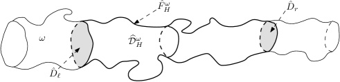
Figure 1: On the definition of finite tube ${\widehat{\mathcal{D}}}^{\omega}_{H}$

Observe that ${\widehat{\mathcal{D}}}^{\omega}_{H}$ can, in fact, consist of several separate pieces, namely, one big piece between $0$ and $H$, and possibly several small pieces near the left and the right ends (we suppose that $H\geq\widetilde{M}$, so that there could not be two or more big pieces). It can be easily seen that those small pieces have no influence on the definition of the transport diffusion coefficient; for notational convention, we still allow ${\widehat{\mathcal{D}}}^{\omega}_{H}$ to be as described above.

Then, we consider a gas of independent particles in ${\widehat{\mathcal{D}}}^{\omega}_{H}$, described as follows. There is usual reflection on ${\hat{F}}^{\omega}_{H}$; any particle which hits ${\hat{D}}_{\ell}\cup{\hat{D}}_{r}$, disappears. In addition, for a given $\lambda>0$, new particles are injected in ${\hat{D}}_{\ell}$ with intensity $(\gamma_{d}|{\mathbb{S}}^{d-1}|)^{-1}\lambda$ per unit surface area. Every newly injected particle chooses the initial direction at random according to the cosine law. In other words, the injection in ${\hat{D}}_{\ell}$ is given by an independent Poisson process in ${\hat{D}}_{\ell}\times{\mathbb{S}}_{\mathbf{e}}$ with intensity $|{\mathbb{S}}^{d-1}|^{-1}\lambda|\mathbf{e}\cdot u|\,dx\,du$.

Remark 2.5

The choice of the cosine law for the injection of new particles is justified by Theorem 2.9 of [6]: for the KSB in a finite domain, the long-run empirical law of intersection with a $(d-1)$-dimensional manifold is cosine. One may think of the following situation: the random tube is connected from its left side ${\hat{D}}_{\ell}$ to a very large reservoir containing the Knudsen gas in the stationary regime; then, the particles cross ${\hat{D}}_{\ell}$ with approximately cosine law (at least on the time scale when the density of the particles in the big reservoir remains unaffected by the outflow through the tube). In Section 4 (proof of Theorem 2.8) we use this kind of argument to obtain a rigorous characterization of the steady state of this gas.

We now consider this gas in the stationary regime. Let $\Xi_{[a,b]}:=[a,b]\times\Xi$, and let ${\mathcal{M}}(a,b)$ be the mean number of particles in ${\widehat{\mathcal{D}}}^{\omega}_{H}\cap\Xi_{[a,b]}$, in a fixed environment $\omega$.

In Theorem 2.6 below we shall see that there exists a constant $\vartheta$ such that

$$\lim_{m\to\infty}\limsup_{H\to\infty}\max_{j=1,\ldots,m}\Bigg{|}\frac{{\mathcal{M}}\big{(}\frac{(m-j)H}{m},\frac{(m-j+1)H}{m}\big{)}}{H/m}-\frac{\vartheta(j-1/2)}{m}\Bigg{|}=0,$$

which means that, after coarse-graining, the particle density profile is asymptotically linear. The above quantity $\vartheta$ is called the (rescaled) density gradient.

We define also the current $J^{\omega}_{H}$ as the mean number of particles absorbed in ${\hat{D}}_{r}$ per unit of time, and let the rescaled current be defined as

$$J=\lim_{H\to\infty}HJ^{\omega}_{H}.$$

Then, consistently with the discussion in the beginning of this section, the transport diffusion coefficient ${\mathsf{D}}_{\text{trans}}$ is defined by

$${\mathsf{D}}_{\text{trans}}=\frac{J}{\vartheta}.$$ (3)

Now, suppose that the quenched invariance principle with constant ${\hat{\sigma}}$ holds for the stochastic billiard. Our goal is to prove that ${\mathsf{D}}_{\text{trans}}$ is equal to the self-diffusion coefficient ${\mathsf{D}}_{\text{self}}:={\hat{\sigma}}^{2}/2$. To this end, we prove the following two results. First, we prove that the coarse-grained density profile is indeed linear:

Theorem 2.6

Suppose that the quenched invariance principle holds. Then, for any $\varepsilon^{\prime}>0$ there exists $m$ such that ${\mathbb{P}}$-a.s.

$$\limsup_{H\to\infty}\max_{j=1,\ldots,m}\Bigg{|}\frac{{\mathcal{M}}\big{(}\frac{(m-j)H}{m},\frac{(m-j+1)H}{m}\big{)}}{H/m}-\frac{\lambda(j-1/2)}{m}\big{\langle}|\omega_{0}|\big{\rangle}_{\!{}_{\mathbb{P}}}\Bigg{|}<\varepsilon^{\prime}$$ (4)

Then, we calculate the limiting current:

Theorem 2.7

Suppose that the quenched invariance principle holds with constant ${\hat{\sigma}}$, and assume also that Condition T holds. Then, we have ${\mathbb{P}}$-a.s.

$$\lim_{H\to\infty}HJ^{\omega}_{H}=\frac{1}{2}\lambda{\hat{\sigma}}^{2}\big{\langle}|\omega_{0}|\big{\rangle}_{\!{}_{\mathbb{P}}}.$$ (5)

Some remarks are in place that illustrate the significance of the above theorems. Theorem 2.6 means that $\vartheta=\lambda\big{\langle}|\omega_{0}|\big{\rangle}_{\!{}_{\mathbb{P}}}$, and using also Theorem 2.7, we obtain that ${\mathsf{D}}_{\text{trans}}={\mathsf{D}}_{\text{self}}$. At the same time it becomes clear that such a statement can be true only asymptotically since in a finite open tube one has to expect finite size corrections of the mean particle number. These corrections may, in fact, depend strongly on the microscopic shape of the tube near the open boundaries. This implies that in experiments on real spatially inhomogeneous systems some care has to be taken as to what is measured as macroscopic density gradient. Notice that with Theorem 2.7 we also prove Fick’s law for diffusive transport of matter in the random Knudsen stochastic billiard. Since the velocity of the particles does not change at collisions with the tube walls, mass transport is proportional to energy transport. In this interpretation Theorem 2.7 implies Fourier’s law for heat conduction, see e.g. [2, 13] for recent work on other processes.

For a function $g\in{\mathcal{C}}[0,\infty)$ and $a\in{\mathbb{R}}$, denote

$$\wp_{a}(g)=\inf\{t\geq 0:g(t)-g(0)=a\}.$$ (6)

As mentioned in the introduction, in the proof of Theorems 2.6 and 2.7 we use the explicit form of the steady state for the Knudsen gas in the random tube with injection from one side. Let us formulate the following theorem:

Theorem 2.8

• For the Knudsen gas with absorption/injection in ${\hat{D}}_{r}\cup{\hat{D}}_{\ell}$ (as before, with intensity $(\gamma_{d}|{\mathbb{S}}^{d-1}|)^{-1}\lambda$ per unit surface area) the unique stationary state is Poisson point process in ${\widehat{\mathcal{D}}}^{\omega}_{H}\times{\mathbb{S}}^{d-1}$ with intensity $\lambda|{\mathbb{S}}^{d-1}|^{-1}$.

• For the gas with injection in ${\hat{D}}_{\ell}$ only, the unique stationary distribution of the particle configuration is given by a Poisson point process in ${\widehat{\mathcal{D}}}^{\omega}_{H}\times{\mathbb{S}}^{d-1}$ with intensity measure

  $$\lambda|{\mathbb{S}}^{d-1}|^{-1}{\mathtt{P}}_{\omega}^{(\alpha,u),-h}[\wp_{-\alpha}(X\cdot e)<\wp_{H-\alpha}(X\cdot\mathbf{e})]\,d\alpha\,du\,dh.$$

Also, in both cases, for any initial configuration the process converges to the stationary state described above.

Of course, the above result is not quite unexpected. It is well known that independent systems have Poisson invariant distributions (with the single particle invariant measure for Poisson intensity), let us mention e.g. [10] (Section VIII.5) and [15]. Still, we decided to include the proof of this theorem because (as far as we know), it does not directly follow from any of the existing results available in the literature.

2.3 Crossing time properties

Let us introduce some more notations for the finite random tube. We denote by ${\tilde{\omega}}_{0}$ the set of points of $\omega_{0}$, from where the particle can reach ${\hat{D}}_{r}$ by a path which stays within ${\widehat{\mathcal{D}}}^{\omega}_{H}$ and set ${\tilde{D}}_{\ell}:=\{0\}\times{\tilde{\omega}}_{0}$ (see Figure 2), and let ${\widetilde{\mathcal{D}}}^{\omega}_{H}\subset{\widehat{\mathcal{D}}}^{\omega}_{H}$ be the corresponding finite tube. Since we are going to study now how long a tagged particle stays inside the tube and how it crosses (i.e., goes to the right boundary without going back to the left boundary), the idea is to inject it in a place from where it can actually do it. Our interest is then in certain first-passage properties, in particular, the total life time of the particle inside ${\widetilde{\mathcal{D}}}^{\omega}_{H}$ (i.e., the time until the particle first exits ${\widetilde{\mathcal{D}}}^{\omega}_{H}$) and the permeation time which the particle needs to first exit ${\widetilde{\mathcal{D}}}^{\omega}_{H}$ at the end of the tube segment “opposite” to that where it was injected, i.e., after crossing the tube.

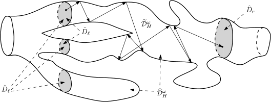
Figure 2: On the definition of ${\tilde{D}}_{\ell},{\widetilde{\mathcal{D}}}^{\omega}_{H}$, and the event ${\mathfrak{C}}_{H}$ (a trajectory crossing the tube is shown)

So, suppose that one particle is injected (uniformly) at random at ${\tilde{D}}_{\ell}$ into the tube ${\widetilde{\mathcal{D}}}^{\omega}_{H}$ (that is, the starting location has the uniform distribution in ${\tilde{D}}_{\ell}$, and the direction is chosen according to the cosine law), and let us denote by ${\mathfrak{C}}_{H}$ the event that it crosses the tube without going back to ${\tilde{D}}_{\ell}$, i.e., ${\mathfrak{C}}_{H}=\{\tau({\hat{D}}_{r})<\tau^{+}({\tilde{D}}_{\ell})\}$ (here, $\tau$ and $\tau^{+}$ are, respectively, entrance and hitting times for the discrete-time process, see (20) and (21) for the precise definitions). Also, define ${\mathcal{T}}_{H}$ to be the total lifetime of the particle, i.e., if $X_{t}$ is the location of the particle at time $t$, then ${\mathcal{T}}_{H}=\min\{t>0:X_{t}\in{\tilde{D}}_{\ell}\cup{\hat{D}}_{r}\}$.

First, we calculate the asymptotic behaviour of the quenched and annealed (averaged) expectation of ${\mathcal{T}}_{H}$:

Theorem 2.9

Suppose that the quenched invariance principle holds with constant ${\hat{\sigma}}$. We have

$$\lim_{H\to\infty}\frac{1}{H}{\mathtt{E}}_{\omega}{\mathcal{T}}_{H} =\frac{\gamma_{d}|{\mathbb{S}}^{d-1}|\big{\langle}|\omega_{0}|\big{\rangle}_{\!{}_{\mathbb{P}}}}{2|{\tilde{\omega}}_{0}|}\qquad\text{${\mathbb{P}}$-a.s.,}$$ (7)

$$\lim_{H\to\infty}\frac{1}{H}\big{\langle}{\mathtt{E}}_{\omega}{\mathcal{T}}_{H}\big{\rangle}_{\!{}_{\mathbb{P}}} =\frac{1}{2}\gamma_{d}|{\mathbb{S}}^{d-1}|\big{\langle}|\omega_{0}|\big{\rangle}_{\!{}_{\mathbb{P}}}\big{\langle}|{\tilde{\omega}}_{0}|^{-1}\big{\rangle}_{\!{}_{\mathbb{P}}}.$$ (8)

Observe that Condition T (i) implies that $|{\tilde{\omega}}_{0}|$ is bounded away from $0$, and so $\big{\langle}|{\tilde{\omega}}_{0}|^{-1}\big{\rangle}_{\!{}_{\mathbb{P}}}<\infty$. At this point we remind the reader that here and in the next theorem the expected “times” are actually expected lengths of flight, related through the corresponding times through the trivial generic relation length$\,=\,$velocity$\times$time. In our Knudsen gas we always assume unit velocity $v=1$ so that times can be identified with the appropriate lengths.

To elucidate the physical significance of Theorem 2.9 we observe that for usual Brownian motion the expected lifetime $T(z_{0})$ of particle in an interval $[0,L]$ is given by $T(z_{0})=z_{0}(L-z_{0})/(2D)$, where $z_{0}$ is the starting position and $D$ is the diffusion coefficient. So, in particular, for a particle starting at the boundary $z_{0}=0$ (or at $z_{0}=L$) the expected life time is $0$. However, in a microscopic model of diffusion in a finite open system, this result cannot be expected to be generally valid because of a positive probability that a particle which starts at $z_{0}=0$ would escape through the other boundary at $L$. Often it is found empirically that the expected life time can be approximated by

$$T(\tilde{z}_{0})=\frac{\tilde{z}_{0}(\tilde{L}-\tilde{z}_{0})}{2D}$$ (9)

with an effective shifted coordinate $\tilde{z}_{0}=z_{0}+\lambda_{M}$ and effective interval length $\tilde{L}=L+2\lambda_{M}$. The empirical shift length $\lambda_{M}$ is known as Milne extrapolation length [4], for a recent application to diffusion in carbon nanotubes see [22]. From the definition (9) one can see that the life time of a particle starting at the origin $z_{0}=0$ allows for the computation of the Milne extrapolation length through the asymptotic relation

$$\lim_{L\to\infty}\frac{T(\lambda_{M})}{L}=\frac{\lambda_{M}}{2D}$$

provided the diffusion coefficient $D$ is known.

In a physical system the Milne extrapolation length depends on molecular details of the gas such as type of molecule or temperature, but in a Knudsen gas also on the tube surface. In our model the properties of the gas are encoded in the unit velocity $v=1$ of the particles. Observe now that the quantity $T(\lambda_{M})$ corresponds to ${\mathtt{E}}_{\omega}{\mathcal{T}}_{H}$ in our setting. Hence, by identifying $H=L$ and using $D=\hat{\sigma}^{2}/2$, Theorem 2.9 furnishes us with the dependence of the Milne extrapolation length on the tube properties through

$$\lambda_{M} =\frac{\gamma_{d}|{\mathbb{S}}^{d-1}|\big{\langle}|\omega_{0}|\big{\rangle}_{\!{}_{\mathbb{P}}}}{2|{\tilde{\omega}}_{0}|}\hat{\sigma}^{2}\qquad\text{${\mathbb{P}}$-a.s.,}$$ (10)

$$\big{\langle}\lambda_{M}\big{\rangle}_{\!{}_{\mathbb{P}}} =\frac{1}{2}\gamma_{d}|{\mathbb{S}}^{d-1}|\big{\langle}|\omega_{0}|\big{\rangle}_{\!{}_{\mathbb{P}}}\big{\langle}|{\tilde{\omega}}_{0}|^{-1}\big{\rangle}_{\!{}_{\mathbb{P}}}\hat{\sigma}^{2}.$$ (11)

Interestingly, $\lambda_{M}$ depends only on very few generic properties of the random tube.

The next result relies on Theorem 2.7, so we need to assume a stronger condition on the geometry of the tube.

Theorem 2.10

Let us suppose that the quenched invariance principle is valid with ${\hat{\sigma}}$, and assume that Condition T holds. For the asymptotics of the probability of crossing, we have

$$\lim_{H\to\infty}H{\mathtt{P}}_{\omega}[{\mathfrak{C}}_{H}]=\frac{\gamma_{d}|{\mathbb{S}}^{d-1}|{\hat{\sigma}}^{2}\big{\langle}|\omega_{0}|\big{\rangle}_{\!{}_{\mathbb{P}}}}{2|{\tilde{\omega}}_{0}|}\qquad\text{${\mathbb{P}}$-a.s.,}$$ (12)

$$\lim_{H\to\infty}H\big{\langle}{\mathtt{P}}_{\omega}[{\mathfrak{C}}_{H}]\big{\rangle}_{\!{}_{\mathbb{P}}}=\frac{1}{2}\gamma_{d}|{\mathbb{S}}^{d-1}|{\hat{\sigma}}^{2}\big{\langle}|\omega_{0}|\big{\rangle}_{\!{}_{\mathbb{P}}}\big{\langle}|{\tilde{\omega}}_{0}|^{-1}\big{\rangle}_{\!{}_{\mathbb{P}}}.$$ (13)

For the quenched behaviour of the conditional expectations, we have, ${\mathbb{P}}$-a.s.

$$\lim_{H\to\infty}\frac{1}{H^{2}}{\mathtt{E}}_{\omega}({\mathcal{T}}_{H}\mid{\mathfrak{C}}_{H}) =\frac{1}{3{\hat{\sigma}}^{2}},$$ (14)

$$\lim_{H\to\infty}\frac{1}{H}{\mathtt{E}}_{\omega}({\mathcal{T}}_{H}{\mathbb{I}}{\{{\mathfrak{C}}_{H}\}}) =\frac{\gamma_{d}|{\mathbb{S}}^{d-1}|\big{\langle}|\omega_{0}|\big{\rangle}_{\!{}_{\mathbb{P}}}}{6|{\tilde{\omega}}_{0}|},$$ (15)

$$\lim_{H\to\infty}\frac{1}{H}{\mathtt{E}}_{\omega}({\mathcal{T}}_{H}{\mathbb{I}}{\{{\mathfrak{C}}_{H}^{c}\}}) =\frac{\gamma_{d}|{\mathbb{S}}^{d-1}|\big{\langle}|\omega_{0}|\big{\rangle}_{\!{}_{\mathbb{P}}}}{3|{\tilde{\omega}}_{0}|},$$ (16)

and for the annealed ones

$$\lim_{H\to\infty}\frac{1}{H^{2}}\big{\langle}{\mathtt{E}}_{\omega}({\mathcal{T}}_{H}\mid{\mathfrak{C}}_{H})\big{\rangle}_{\!{}_{\mathbb{P}}} =\frac{1}{3{\hat{\sigma}}^{2}},$$ (17)

$$\lim_{H\to\infty}\frac{1}{H}{\mathtt{E}}_{\omega}({\mathcal{T}}_{H}{\mathbb{I}}{\{{\mathfrak{C}}_{H}\}}) =\frac{1}{6}\gamma_{d}|{\mathbb{S}}^{d-1}|\big{\langle}|\omega_{0}|\big{\rangle}_{\!{}_{\mathbb{P}}}\big{\langle}|{\tilde{\omega}}_{0}|^{-1}\big{\rangle}_{\!{}_{\mathbb{P}}},$$ (18)

$$\lim_{H\to\infty}\frac{1}{H}{\mathtt{E}}_{\omega}({\mathcal{T}}_{H}{\mathbb{I}}{\{{\mathfrak{C}}_{H}^{c}\}}) =\frac{1}{3}\gamma_{d}|{\mathbb{S}}^{d-1}|\big{\langle}|\omega_{0}|\big{\rangle}_{\!{}_{\mathbb{P}}}\big{\langle}|{\tilde{\omega}}_{0}|^{-1}\big{\rangle}_{\!{}_{\mathbb{P}}}.$$ (19)

As one sees from Theorems 2.9 and 2.10, all our annealed results in fact say that one can interchange the limit as $H\to\infty$ with integration with respect to ${\mathbb{P}}$. We still decided to include these results (even though they are technically not difficult) because, in models related to random environment, it is frequent that the annealed behaviour differs substantially from the quenched behaviour.

One may find it interesting to observe that, by (15) and (16)

$$\frac{{\mathtt{E}}_{\omega}({\mathcal{T}}_{H}{\mathbb{I}}{\{{\mathfrak{C}}_{H}^{c}\}})}{{\mathtt{E}}_{\omega}({\mathcal{T}}_{H}{\mathbb{I}}{\{{\mathfrak{C}}_{H}\}})}\to 2\quad\text{ as }H\to\infty.$$

To obtain another interesting consequence of our results, let us suppose now that ${\mathbb{P}}$-a.s. the random tube is such that we have $|{\tilde{\omega}}_{0}|=|\omega_{0}|$. Observe that, by Jensen’s inequality, it holds that

$$\big{\langle}|\omega_{0}|\big{\rangle}_{\!{}_{\mathbb{P}}}\big{\langle}|\omega_{0}|^{-1}\big{\rangle}_{\!{}_{\mathbb{P}}}\geq 1$$

(and the inequality is strict if the distribution of $|\omega_{0}|$ is nondegenerate), so “roughness” of the tube makes the quantities $\big{\langle}{\mathtt{E}}_{\omega}{\mathcal{T}}_{H}\big{\rangle}_{\!{}_{\mathbb{P}}}$ and $\big{\langle}{\mathtt{E}}_{\omega}({\mathcal{T}}_{H}{\mathbb{I}}{\{{\mathfrak{C}}_{H}\}})\big{\rangle}_{\!{}_{\mathbb{P}}}$ increase. In other words, these quantities as well as the Milne correlation length are minimized on the tubes with constant section (which, by the way, do not have to be necessarily “straight cylinders”!).

The remaining part of the paper is devoted to the proofs of our results, and, as mentioned in the introduction, it is organized in the following way. In Section 3 we obtain several auxiliary results related to hitting of sets by the random billiard. In Section 4 we obtain the explicit form of the stationary measure of the Knudsen gas in the finite tube ${\widehat{\mathcal{D}}}^{\omega}_{H}$ by using the corresponding result from [6] about the stationary distribution of one particle in a finite domain. Then, in Section 5.1, we apply the results of Sections 3 and 4 to obtain the explicit form of the transport diffusion coefficient. Finally, in Section 5.2 we use Little’s theorem to prove the results related to the crossing time of the random tube.

3 Some preliminary facts: hitting times and estimates on the crossing probabilities

We need first to prove several auxiliary facts for random billiard in arbitrary finite domains. As in [6], let ${\mathcal{D}}$ be a bounded domain with Lipschitz and a.e. continuously differentiable boundary. We keep the notation ${\mathtt{P}}_{\omega}$ to denote the law of our processes, and we still use $\nu^{\omega}$ to denote the $(d-1)$-dimensional Hausdorff measure on the boundary $\partial{\mathcal{D}}$. Consider a Markov chain $\bar{\xi}$ on $\partial{\mathcal{D}}$, which has a transition density $\bar{K}$ with the property ${\bar{K}}(x,y)={\bar{K}}(y,x)$ for all $x,y\in\partial{\mathcal{D}}$. Observe that the Knudsen random walk $\xi$ has the above property, but we need to formulate the next results in a slightly more general framework, since we shall need to apply them to some other processes built upon $\xi$. Let us introduce the notations

$$\tau(B) =\min\{n\geq 0:\bar{\xi}_{n}\in B\},$$ (20)

$$\tau^{+}(B) =\min\{n\geq 1:\bar{\xi}_{n}\in B\}$$ (21)

for the entrance and the hitting time of $B\subset\partial{\mathcal{D}}$. Also, for measurable $B\subset\partial\omega$ such that $0<\nu^{\omega}(B)<\infty$ we shall write

$${\mathtt{P}}_{\omega}^{B}[\cdot]=\frac{1}{\nu^{\omega}(B)}\int\limits_{B}{\mathtt{P}}_{\omega}^{x}[\cdot]\,d\nu^{\omega}(x),$$

so that ${\mathtt{P}}_{\omega}^{B}$ is the law for the process starting from the uniform distribution on $B$.

Taking advantage of the reversibility of the process $\xi$, we prove the following

Lemma 3.1

Consider two arbitrary measurable sets $B,F\subset\partial{\mathcal{D}}$ such that $B\cap F=\emptyset$.

• Suppose that $\nu^{\omega}(B),\nu^{\omega}(F)\in(0,+\infty)$. For any $F^{\prime}\subset F$, we have

  $${\mathtt{P}}_{\omega}^{B}[\xi_{\tau(F)}\in F^{\prime}\mid\tau(F)<\tau^{+}(B)]$$

  $$=\frac{1}{\nu^{\omega}(B){\mathtt{P}}_{\omega}^{B}[\tau(F)<\tau^{+}(B)]}\int\limits_{F^{\prime}}{\mathtt{P}}_{\omega}^{y}[\tau(B)<\tau^{+}(F)]\,d\nu^{\omega}(y)$$

  $$=\frac{1}{\nu^{\omega}(F){\mathtt{P}}_{\omega}^{F}[\tau(B)<\tau^{+}(F)]}\int\limits_{F^{\prime}}{\mathtt{P}}_{\omega}^{y}[\tau(B)<\tau^{+}(F)]\,d\nu^{\omega}(y).$$ (22)

• Suppose that $\nu^{\omega}(B)\in(0,+\infty)$. For any $B^{\prime},B^{\prime\prime}\subset B$, we have

  $$\int\limits_{B^{\prime}}{\mathtt{P}}_{\omega}^{x}[\xi_{\tau^{+}(B)}\in B^{\prime\prime},\tau^{+}(B)<\tau(F)]\,d\nu^{\omega}(x)$$

  $$=\int\limits_{B^{\prime\prime}}{\mathtt{P}}_{\omega}^{x}[\xi_{\tau^{+}(B)}\in B^{\prime},\tau^{+}(B)<\tau(F)]\,d\nu^{\omega}(x).$$ (23)

One immediately obtains the following consequence of Lemma 3.1 (ii):

Corollary 3.2

For any $B,F\subset\partial{\mathcal{D}}$ such that $B\cap F=\emptyset$ and $\nu^{\omega}(B)\in(0,+\infty)$, we have the following.

• For $x,y\in B$, let us define the conditional (on the event $\{\tau^{+}(B)<\tau(F)\}$) transition density ${\bar{K}}_{B,F}(x,y)$:

  $${\mathtt{P}}_{\omega}^{x}[\xi_{\tau^{+}(B)}\in B^{\prime\prime}\mid\tau^{+}(B)<\tau(F)]=\int\limits_{B^{\prime\prime}}{\bar{K}}_{B,F}(x,y)\,d\nu^{\omega}(y).$$

  Then, we have

  $${\mathtt{P}}_{\omega}^{x}[\tau^{+}(B)<\tau(F)]{\bar{K}}_{B,F}(x,y)={\mathtt{P}}_{\omega}^{y}[\tau^{+}(B)<\tau(F)]{\bar{K}}_{B,F}(y,x),$$

  that is, the random walk conditioned to return to $B$ without hitting $F$ is reversible with the reversible measure $\nu^{\omega}_{B,F}$ defined by

  $$\frac{d\nu^{\omega}_{B,F}}{d\nu^{\omega}}(x)={\mathtt{P}}_{\omega}^{x}[\tau^{+}(B)<\tau(F)].$$

• In particular (take $F=\emptyset$ in the previous part) the random walk observed at the moments of successive visits to $B$ is reversible with the reversible measure $\nu^{\omega}$.

Proof of Lemma 3.1. Abbreviate for the moment $U:={\mathcal{D}}\setminus(B\cup F)$. First, write using the fact that ${\bar{K}}$ is symmetric

$${\mathtt{P}}_{\omega}^{B}[\tau(F)<\tau^{+}(B)] =\sum_{n=1}^{\infty}{\mathtt{P}}_{\omega}^{B}[\tau(F)=n,\tau^{+}(B)>n]$$

$$=\sum_{n=1}^{\infty}\int\limits_{B}\frac{d\nu^{\omega}(x_{0})}{\nu^{\omega}(B)}\int\limits_{U^{n-1}}d\nu^{\omega}(x_{1})\ldots d\nu^{\omega}(x_{n-1})$$

$$\qquad\qquad\times\int\limits_{F}d\nu^{\omega}(x_{n}){\bar{K}}(x_{0},x_{1})\ldots{\bar{K}}(x_{n-1},x_{n})$$

$$=\frac{\nu^{\omega}(F)}{\nu^{\omega}(B)}\sum_{n=1}^{\infty}\int\limits_{F}\frac{d\nu^{\omega}(x_{n})}{\nu^{\omega}(F)}\int\limits_{U^{n-1}}d\nu^{\omega}(x_{n-1})\ldots d\nu^{\omega}(x_{1})$$

$$\qquad\qquad\times\int\limits_{B}d\nu^{\omega}(x_{0}){\bar{K}}(x_{n},x_{n-1})\ldots{\bar{K}}(x_{1},x_{0})$$

$$=\frac{\nu^{\omega}(F)}{\nu^{\omega}(B)}\sum_{n=1}^{\infty}{\mathtt{P}}_{\omega}^{F}[\tau(B)=n,\tau^{+}(F)>n]$$

$$=\frac{\nu^{\omega}(F)}{\nu^{\omega}(B)}{\mathtt{P}}_{\omega}^{F}[\tau(B)<\tau^{+}(F)].$$

Then, similarly

$${\mathtt{P}}_{\omega}^{B}[\xi_{\tau(F)}\in F^{\prime}\mid\tau(F)<\tau^{+}(B)]$$

$$=\frac{1}{{\mathtt{P}}_{\omega}^{B}[\tau(F)<\tau^{+}(B)]}\sum_{n=1}^{\infty}{\mathtt{P}}_{\omega}^{B}[\tau(F)=n,\xi_{\tau(F)}\in F^{\prime},\tau^{+}(B)>n]$$

$$=\frac{\nu^{\omega}(B)}{\nu^{\omega}(F){\mathtt{P}}_{\omega}^{F}[\tau(B)<\tau^{+}(F)]}\sum_{n=1}^{\infty}\int\limits_{B}\frac{d\nu^{\omega}(x_{0})}{\nu^{\omega}(B)}\int\limits_{U^{n-1}}d\nu^{\omega}(x_{1})\ldots d\nu^{\omega}(x_{n-1})$$

$$\qquad\qquad\qquad\qquad\qquad\qquad\qquad\times\int\limits_{F^{\prime}}d\nu^{\omega}(x_{n}){\bar{K}}(x_{0},x_{1})\ldots{\bar{K}}(x_{n-1},x_{n})$$

$$=\frac{1}{\nu^{\omega}(F){\mathtt{P}}_{\omega}^{F}[\tau(B)<\tau^{+}(F)]}\int\limits_{F^{\prime}}{\mathtt{P}}_{\omega}^{y}[\tau(B)<\tau^{+}(F)]\,d\nu^{\omega}(y),$$

so (22) is proved.

Let us prove (23). Analogously to the previous computation, we write

$$\int\limits_{B^{\prime}}{\mathtt{P}}_{\omega}^{x}[\xi_{\tau^{+}(B)}\in B^{\prime\prime},\tau^{+}(B)<\tau(F)]\,d\nu^{\omega}(x)$$

$$=\int\limits_{B^{\prime}}d\nu^{\omega}(x)\sum_{n=1}^{\infty}{\mathtt{P}}_{\omega}^{x}[\xi_{\tau^{+}(B)}\in B^{\prime\prime},\tau^{+}(B)=n,\tau(F)>n]$$

$$=\sum_{n=1}^{\infty}\int\limits_{B^{\prime}}d\nu^{\omega}(x_{0})\int\limits_{U^{n-1}}d\nu^{\omega}(x_{1})\ldots d\nu^{\omega}(x_{n-1})$$

$$\qquad\qquad\times\int\limits_{B^{\prime\prime}}d\nu^{\omega}(x_{n}){\bar{K}}(x_{0},x_{1})\ldots{\bar{K}}(x_{n-1},x_{n})$$

$$=\sum_{n=1}^{\infty}\int\limits_{B^{\prime\prime}}d\nu^{\omega}(x_{n})\int\limits_{U^{n-1}}d\nu^{\omega}(x_{n-1})\ldots d\nu^{\omega}(x_{1})$$

$$\qquad\qquad\times\int\limits_{B^{\prime}}d\nu^{\omega}(x_{0}){\bar{K}}(x_{n},x_{n-1})\ldots{\bar{K}}(x_{1},x_{0})$$

$$=\int\limits_{B^{\prime\prime}}{\mathtt{P}}_{\omega}^{x}[\xi_{\tau^{+}(B)}\in B^{\prime},\tau^{+}(B)<\tau(F)]\,d\nu^{\omega}(x),$$

and (23) is proved. This concludes the proof of Lemma 3.1. $\Box$

Next, we recall the Dirichlet’s principle:

Proposition 3.3

Consider $B,F\subset\partial{\mathcal{D}}$ with $B\cap F=\emptyset$ and $\nu^{\omega}(B)\in(0,+\infty)$, and denote ${\hat{h}}(x)={\mathtt{P}}_{\omega}^{x}[\tau(F)<\tau(B)]$ (so that, in particular, ${\hat{h}}(x)=0$ for all $x\in B$ and ${\hat{h}}(x)=1$ for all $x\in F$). Define

$${\mathcal{H}}=\{h:h(x)\in[0,1],h(x)=0\text{ for all }x\in B,h(x)=1\text{ for all }x\in F\}.$$

Then

$$2\nu^{\omega}(B){\mathtt{P}}_{\omega}^{B}[\tau(F)<\tau^{+}(B)]={\mathcal{E}}({\hat{h}},{\hat{h}})=\min_{h\in{\mathcal{H}}}{\mathcal{E}}(h,h),$$ (24)

where

$${\mathcal{E}}(h,h)=\int\limits_{(\partial{\mathcal{D}})^{2}}{\bar{K}}(x,y)(h(x)-h(y))^{2}\,d\nu^{\omega}(x)\,d\nu^{\omega}(y).$$ (25)

Proof. For the proof, we refer to the discrete case, e.g. Proposition 3.8 in [1], and observe that the proof applies to the space-continuous case, using that, on general spaces, harmonicity in the analytic sense and in the probabilistic sense are equivalent notions by [5]. Indeed, minimizers $h$ of the Dirichlet form are harmonic in the analytic sense, i.e., there are in the kernel of the form (see (2.10) in [5]), though the left-hand side of (24) is the value of ${\mathcal{E}}(h,h)$ when $h$ is harmonic in the probabilistic sense, i.e., the expectation of the process at some exit time (see Theorem 2.7 in [5]) with the appropriate boundary conditions. $\Box$

Now, we go back to the Knudsen random walk in the random tube $\omega$. Recall that $K^{n}$ stands for the the $n$-step transition density of KRW, and that we have $K^{n}(x,y)=K^{n}(y,x)$ for all $x,y$.

Let us define for an arbitrary $A\subset{\mathbb{R}}$

$${\tilde{F}}^{\omega}(A)=\{x\in\partial\omega:x\cdot e\in A\}.$$

In case $A$ is an interval, say, $A=[a,b)$, we write ${\tilde{F}}^{\omega}[a,b)$ instead of ${\tilde{F}}^{\omega}([a,b))$. There is the following apriory bound on the size of the jump of the random billiard: there exists a constant ${\tilde{\gamma}}_{1}>0$, depending only on ${\widehat{M}}={\mathop{\rm diam}}(\Xi)/2$ and the dimension, such that for ${\mathbb{P}}$-almost all $\omega$

$${\mathtt{P}}_{\omega}[|(\xi_{1}-\xi_{0})\cdot\mathbf{e}|\geq u\mid\xi_{0}=x]\leq{\tilde{\gamma}}_{1}u^{-(d-1)},$$ (26)

for all $x\in\partial\omega$, $u\geq 1$, see formula (54) of [7]. Moreover, using (26), for any $n\geq 1$ it is straightforward to obtain that, for some ${\tilde{\gamma}}^{(n)}_{1}>0$

$${\mathtt{P}}_{\omega}[|(\xi_{n}-\xi_{0})\cdot\mathbf{e}|\geq u\mid\xi_{0}=x]\leq{\tilde{\gamma}}^{(n)}_{1}u^{-(d-1)},$$ (27)

for all $x\in\partial\omega$, $u\geq 1$ (also, without restriction of generality, we can assume that ${\tilde{\gamma}}^{(n)}_{1}$ is nondecreasing in $n$).

Now, with the help of the above formula we prove the following result:

Lemma 3.4

For any $n\geq 1$ there exists ${\tilde{\gamma}}^{(n)}_{2}>0$ such that for all $u\geq 1$ and $a\in{\mathbb{R}}$ we have

$$\int\limits_{{\tilde{F}}^{\omega}(-\infty,a)}d\nu^{\omega}(x)\int\limits_{{\tilde{F}}^{\omega}(a+u,\infty)}d\nu^{\omega}(y)K^{n}(x,y)\leq{\tilde{\gamma}}^{(n)}_{2}u^{-(d-1)}.$$ (28)

Proof. Abbreviate $V=\{a+u\}\times\omega_{a+u}$. The main idea is the following: if at some step the Knudsen random walk jumped from some point of ${\tilde{F}}^{\omega}(-\infty,a+u)$ to ${\tilde{F}}^{\omega}[a+u,\infty)$, it must cross $V$, so the probability of such a jump is the same as the probability of the jump to $V$ in the semi-infinite tube with the boundary ${\tilde{F}}^{\omega}(-\infty,a+u)\cup V$. So, we obtain

$$\int\limits_{{\tilde{F}}^{\omega}(-\infty,a]}d\nu^{\omega}(x)\int\limits_{{\tilde{F}}^{\omega}[a+u,\infty)}d\nu^{\omega}(y)K^{n}(x,y)$$

$$=\int\limits_{{\tilde{F}}^{\omega}(-\infty,a]}{\mathtt{P}}_{\omega}^{x}[\xi_{n}\in{\tilde{F}}^{\omega}[a+u,\infty)]\,d\nu^{\omega}(x)$$

$$\leq\int\limits_{{\tilde{F}}^{\omega}(-\infty,a]}{\mathtt{P}}_{\omega}^{x}\Big{[}\bigcup_{k=1}^{n}\{\xi_{k}\cdot\mathbf{e}\geq a+u,\xi_{j}\cdot\mathbf{e}<a+u\text{ for all }j<k\}\Big{]}\,d\nu^{\omega}(x)$$

$$\leq\int\limits_{{\tilde{F}}^{\omega}(-\infty,a]}d\nu^{\omega}(x_{0})\sum_{k=1}^{n}\int\limits_{({\tilde{F}}^{\omega}(-\infty,a+u))^{k-1}}d\nu^{\omega}(x_{0})\ldots d\nu^{\omega}(x_{k-1})$$

$$\qquad\qquad\qquad\qquad\qquad\qquad\int\limits_{{\tilde{F}}^{\omega}[a+u,\infty)}d\nu^{\omega}(x_{k})K(x_{0},x_{1})\ldots K(x_{k-1},x_{k})$$

$$\leq\int\limits_{{\tilde{F}}^{\omega}(-\infty,a]}d\nu^{\omega}(x)\int\limits_{V}d\nu^{\omega}(y)\big{(}K(x,y)+K^{2}(x,y)+\cdots+K^{n}(x,y)\big{)}.$$

By symmetry of $K$, we have for any $m$

$$\int\limits_{{\tilde{F}}^{\omega}(-\infty,a)}d\nu^{\omega}(x)\int\limits_{V}d\nu^{\omega}(y)K^{m}(x,y)=\int\limits_{V}{\mathtt{P}}_{\omega}^{y}[\xi_{m}\cdot\mathbf{e}<a]\,d\nu^{\omega}(y),$$

so Lemma 3.4 now follows from (27). $\Box$

Let us consider a sequence of i.i.d. random variables $Z_{1},Z_{2},Z_{3},\ldots$ with uniform distribution on $\{1,2,\ldots,N\}$ (where $N$ is from Condition T (ii)), independent of everything. Also, let us define ${\hat{\xi}}_{n}:=\xi_{Z_{1}+\cdots+Z_{n}}$. Then, it is straightforward to obtain that, for any $x\in\partial\omega$ and $B\subset\{y\in\partial\omega:-1\leq(y-x)\cdot\mathbf{e}\leq 1\}$, we have

$${\mathtt{P}}_{\omega}^{x}[\hat{\xi}_{1}\in B]\geq N^{-1}r_{1}\nu^{\omega}(B)$$ (29)

for some $r_{1}>0$. Let

$${\hat{K}}(x,y)=\frac{1}{N}\sum_{j=1}^{N}K^{j}(x,y)$$

be the transition density of the process $({\hat{\xi}}_{n},n\geq 0)$. Observe that this process is still reversible with the reversible measure $\nu^{\omega}$, so that ${\hat{K}}(x,y)={\hat{K}}(y,x)$ for all $x,y\in\partial\omega$. Similarly to [7], let us define

$$b(x) ={\mathtt{E}}_{\omega}^{x}((\xi_{1}-x)\cdot\mathbf{e})^{2}$$

$$=\int\limits_{\partial\omega}((y-x)\cdot\mathbf{e})^{2}K(x,y)\,\nu^{\omega}(y),$$ (30)

and

$${\hat{b}}(x) ={\mathtt{E}}_{\omega}^{x}((\xi_{Z_{1}}-x)\cdot\mathbf{e})^{2}$$

$$=\int\limits_{\partial\omega}((y-x)\cdot\mathbf{e})^{2}{\hat{K}}(x,y)\,\nu^{\omega}(y).$$ (31)

We suppose that $\tau(B)$ and $\tau^{+}(B)$ are defined as in (20)–(21) but with $\xi$ instead of $\bar{\xi}$, and let ${\hat{\tau}}(B)$ and ${\hat{\tau}}^{+}(B)$ be the corresponding quantities for the process $\hat{\xi}$.

Lemma 3.5

Suppose that $B,F\subset\partial\omega$ with $\nu^{\omega}(B)\in(0,\infty)$. Moreover, assume that $x\cdot\mathbf{e}\leq a$ for all $x\in B$, and $y\cdot\mathbf{e}\geq a+u$ for all $y\in F$ (of course, the same result is valid if we assume that $x\cdot\mathbf{e}\leq a$ for all $x\in F$, and $y\cdot\mathbf{e}\geq a+u$ for all $y\in B$). Then, there exist positive constants ${\tilde{\gamma}}_{3}$, ${\tilde{\gamma}}_{4}$, such that

$$\nu^{\omega}(B){\mathtt{P}}_{\omega}^{B}[\tau(F)<\tau^{+}(B)]\leq{\tilde{\gamma}}_{3}u^{-(d-1)}+\frac{1}{u^{2}}\int\limits_{{\tilde{F}}^{\omega}[a,a+u]}b(x)\,d\nu^{\omega}(x),$$ (32)

and

$$\nu^{\omega}(B){\mathtt{P}}_{\omega}^{B}[\hat{\tau}(F)<\hat{\tau}^{+}(B)]\leq{\tilde{\gamma}}_{4}u^{-(d-1)}+\frac{1}{u^{2}}\int\limits_{{\tilde{F}}^{\omega}[a,a+u]}{\hat{b}}(x)\,d\nu^{\omega}(x).$$ (33)

Moreover, (32) and (33) are valid also in the finite tube ${\widehat{\mathcal{D}}}^{\omega}_{H}$ (in this case we assume that $a>0$ and $a+u<H$).

Proof. We keep the notation ${\mathcal{E}}(\cdot,\cdot)$ for the Dirichlet’s form with respect to $K$, defined as in (25). Suppose without restriction of generality that $a=0$ and define the function

$$h(x)=\begin{cases}0,&\text{ if }x\cdot\mathbf{e}\leq 0,\\ 1,&\text{ if }x\cdot\mathbf{e}\geq u,\\ u^{-1}(x\cdot\mathbf{e}),&\text{ if }x\cdot\mathbf{e}\in(0,u).\end{cases}$$

Using Proposition 3.3 (observe that $h\in\mathcal{H}$) and Lemma 3.4, we obtain

$$2\nu^{\omega}(B){\mathtt{P}}_{\omega}^{B}[\tau(F)<\tau^{+}(B)]$$

$$\leq{\mathcal{E}}(h,h)$$

$$=\int\limits_{(\partial\omega)^{2}}d\nu^{\omega}(x)\,d\nu^{\omega}(y)K(x,y)(h(x)-h(y))^{2}$$

$$=2\int\limits_{{\tilde{F}}^{\omega}(-\infty,0)}d\nu^{\omega}(x)\int\limits_{{\tilde{F}}^{\omega}(u,\infty)}d\nu^{\omega}(y)K(x,y)$$

$$\quad+u^{-2}\int\limits_{({\tilde{F}}^{\omega}[0,u])^{2}}d\nu^{\omega}(x)\,d\nu^{\omega}(y)K(x,y)((y-x)\cdot\mathbf{e})^{2}$$

$$\quad+2u^{-2}\int\limits_{{\tilde{F}}^{\omega}[0,u]}d\nu^{\omega}(x)\int\limits_{{\tilde{F}}^{\omega}(-\infty,0)}d\nu^{\omega}(y)K(x,y)(x\cdot\mathbf{e})^{2}$$

$$\quad+2\int\limits_{{\tilde{F}}^{\omega}[0,u]}d\nu^{\omega}(x)\int\limits_{{\tilde{F}}^{\omega}(u,\infty)}d\nu^{\omega}(y)K(x,y)(1-u^{-1}x\cdot\mathbf{e})^{2}$$

$$\leq 2{\tilde{\gamma}}_{3}u^{-(d-1)}+2u^{-2}\int\limits_{{\tilde{F}}^{\omega}[0,u]}d\nu^{\omega}(x)\int\limits_{\partial\omega}d\nu^{\omega}(y)K(x,y)((y-x)\cdot\mathbf{e})^{2}$$

$$=2{\tilde{\gamma}}_{3}u^{-(d-1)}+\frac{1}{u^{2}}\int\limits_{{\tilde{F}}^{\omega}[a,a+u]}b(x)\,d\nu^{\omega}(x),$$

and this proves (32). The proof of (33) is completely analogous. $\Box$

We now work in finite tube ${\widehat{\mathcal{D}}}^{\omega}_{H}$. Let us use the abbreviations $U_{n}={\tilde{F}}^{\omega}[n-1,n)$, and $V_{n}={\tilde{F}}^{\omega}[n,H)\cup{\hat{D}}_{r}$. Observe that, by Condition T (i), we have that for some ${\tilde{\gamma}}_{5}\in(0,+\infty)$

$$\nu^{\omega}(U_{n})\geq{\tilde{\gamma}}_{5}$$ (34)

for all $n$ and for ${\mathbb{P}}$-a.a. $\omega$.

To distinguish between the seconds moments of the projected jump length in finite and infinite tubes, we modify our notations in the following way. For $x\in\partial{\widehat{\mathcal{D}}}^{\omega}_{H}$, let $b_{H}(x)$ and ${\hat{b}}_{H}(x)$ be the quantities defined as in (30) and (31), but in the finite tube ${\widehat{\mathcal{D}}}^{\omega}_{H}$. Let us use the notations $b_{\infty}(x)$ and ${\hat{b}}_{\infty}(x)$ for the corresponding quantities in the infinite tube. Now, we need an estimate on the integrals appearing in the right-hand sides of (32) and (33), for the case of the finite tube:

Lemma 3.6

Suppose that $0<s_{1}<s_{2}<1$ and assume that $d\geq 3$ and Condition T holds. Then, we have

$$\limsup_{H\to\infty}\frac{1}{H}\int\limits_{{\tilde{F}}^{\omega}[s_{1}H,s_{2}H]}b_{H}(x)\,d\nu^{\omega}(x)<\infty\qquad{\mathbb{P}}\text{-a.s.},$$ (35)

and the same is valid with ${\hat{b}}_{H}$ on the place of $b_{H}$.

Proof. Let us recall some notations from [7]. Define

$${\mathfrak{S}}=\{(\omega,u):\omega\in\Omega,u\in\partial\omega_{0}\}.$$

Define the probability measure ${\mathbb{Q}}$ on ${\mathfrak{S}}$ by

$$d{\mathbb{Q}}(\omega,u)=\frac{1}{{\mathcal{Z}}}\kappa_{0,u}^{-1}\,d\mu^{\omega}_{0}(u)\,d{\mathbb{P}}(\omega),$$ (36)

where $\mu^{\omega}_{0}$ is the $(d-2)$-dimensional Hausdorff measure on the boundary of $\omega_{0}$, $\kappa_{0,u}$ is the scalar product of the normal vectors pointing inside the section and inside the tube (see Section 2 of [7] for details), and ${\mathcal{Z}}=\int_{\Omega}d{\mathbb{P}}\int_{\Xi}\kappa_{0,u}^{-1}d\mu^{\omega}_{0}(u)$ is the normalizing constant. In Lemma 3.1 of [7] it is shown that ${\mathbb{Q}}$ is the invariant law of the environment seen from the walker, that is

$$\big{\langle}{\mathtt{E}}_{\omega}[f(\theta_{\xi_{n}\cdot\mathbf{e}}\omega,{\mathcal{U}}\xi_{n})\mid\xi_{0}=(0,u)]\big{\rangle}_{\!{}_{\mathbb{Q}}}=\big{\langle}f\big{\rangle}_{\!{}_{\mathbb{Q}}}.$$ (37)

Using also that

$${\mathtt{E}}_{\omega}^{x}((\xi_{n}-x))^{2}\leq n\sum_{k=1}^{n}{\mathtt{E}}_{\omega}^{x}((\xi_{k}-\xi_{k-1}))^{2}$$

and (37), it is straightforward to obtain that $\big{\langle}b_{\infty}\big{\rangle}_{\!{}_{\mathbb{Q}}}<\infty$ implies $\big{\langle}{\hat{b}}_{\infty}\big{\rangle}_{\!{}_{\mathbb{Q}}}<\infty$. So, using the notations of [7], by the ergodic theorem we obtain

$$\frac{1}{H}\int\limits_{{\tilde{F}}^{\omega}[0,H]}b_{\infty}(x)\,d\nu^{\omega}(x) =\frac{1}{H}\int\limits_{0}^{H}d\alpha\int\limits_{\Xi}d\mu^{\omega}_{\alpha}(v)\kappa^{-1}_{\alpha,v}b_{\infty}(\theta_{\alpha}\omega,v)$$

$$\to\big{\langle}b_{\infty}\big{\rangle}_{\!{}_{\mathbb{Q}}}\qquad\text{as $H\to\infty$},$$ (38)

a.s. and in $L^{1}$, and the same with ${\hat{b}}_{\infty}$ on the place of $b_{\infty}$. Then, (35) follows from the fact that, for all $H$, $b_{H}(x)\leq b_{\infty}(x)$ for all $x\in{\hat{F}}^{\omega}_{H}$. Now, with ${\hat{b}}_{\infty}$ instead of $b_{\infty}$, the previous inequality is not necessarily valid. So, to prove (35) for ${\hat{b}}_{H}$ instead of $b_{H}$, consider $x\in\partial\omega$ such that $H^{-1}(x\cdot\mathbf{e})\in[s_{1},s_{2}]$, and write (note that for all $x\in\partial{\widehat{\mathcal{D}}}^{\omega}_{H}$ we have ${\hat{b}}_{H}(x)\leq H^{2}$)

$$\big{|}{\hat{b}}_{H}(x)-{\hat{b}}_{\infty}(x)\big{|} \leq H^{2}{\mathtt{P}}_{\omega}^{x}\big{[}\max_{k\leq N}|(\xi_{k}-x)\cdot\mathbf{e}|\geq(s_{1}\wedge(1-s_{2}))H^{-(d-1)}\big{]}$$

$$\leq C_{1}H^{-(d-3)}$$

(recall that $d\geq 3$), and then we obtain (35) for ${\hat{b}}_{H}$ as well. $\Box$

Next, we obtain a lower bound for certain escape probabilities:

Lemma 3.7

Suppose that $H/4\leq n\leq H-1$, and $m<n$. Also, assume that $d\geq 3$ and Condition T holds. Then, there exist positive constants ${\tilde{\gamma}}_{7}$, ${\tilde{\gamma}}_{8}$, such that

$${\mathtt{P}}_{\omega}^{U_{m}}[\hat{\tau}(V_{n})<{\hat{\tau}}^{+}(U_{m})]\geq\frac{{\tilde{\gamma}}_{7}}{n-m},$$ (39)

and

$${\mathtt{P}}_{\omega}^{{\hat{D}}_{\ell}}[\hat{\tau}(V_{n})<{\hat{\tau}}^{+}({\hat{D}}_{\ell})]\geq\frac{{\tilde{\gamma}}_{8}}{H}.$$ (40)

Proof. Let $\hat{\mathcal{E}}$ be the Dirichlet form corresponding to $\hat{K}$ (cf. (25)). First, let us prove (39). As in Proposition 3.3, we use the notation ${\hat{h}}(x)={\mathtt{P}}_{\omega}^{x}[\hat{\tau}(V_{n})<{\hat{\tau}}(U_{m})]$; observe that ${\hat{h}}(x)=0$ for all $x\in U_{m}$ and ${\hat{h}}(y)=1$ for all $y\in V_{n}$ (and hence for all $y\in U_{n+1}$). Using this fact together with (34) and Cauchy-Schwarz inequality, we write (abbreviating $u:=n-m$)

$$2\nu^{\omega}(U_{m}){\mathtt{P}}_{\omega}^{U_{m}}[\hat{\tau}(V_{n})<{\hat{\tau}}^{+}(U_{m})]$$

$$={\hat{\mathcal{E}}}({\hat{h}},{\hat{h}})$$

$$\geq\sum_{j=0}^{u}\int\limits_{U_{m+j}}d\nu^{\omega}(x_{j})\int\limits_{U_{m+j+1}}d\nu^{\omega}(x_{j+1}){\hat{K}}(x_{j},x_{j+1})({\hat{h}}(x_{j})-{\hat{h}}(x_{j+1}))^{2}$$

$$=\Big{(}\prod_{j=0}^{u+1}\nu^{\omega}(U_{m+j})\Big{)}^{-1}\int\limits_{U_{m}}d\nu^{\omega}(x_{0})\ldots\int\limits_{U_{m+u+1}}d\nu^{\omega}(x_{u+1})$$

$$\qquad\qquad\qquad\sum_{j=0}^{u}\nu^{\omega}(U_{m+j})\nu^{\omega}(U_{m+j+1}){\hat{K}}(x_{j},x_{j+1})({\hat{h}}(x_{j})-{\hat{h}}(x_{j+1}))^{2}$$

$$\geq N^{-1}r_{1}{\tilde{\gamma}}_{5}^{2}\Big{(}\prod_{j=0}^{u+1}\nu^{\omega}(U_{m+j})\Big{)}^{-1}\int\limits_{U_{m}}d\nu^{\omega}(x_{0})\ldots$$

$$\qquad\qquad\qquad\ldots\int\limits_{U_{m+u+1}}d\nu^{\omega}(x_{u+1})\sum_{j=0}^{u}({\hat{h}}(x_{j})-{\hat{h}}(x_{j+1}))^{2}$$

$$\geq\frac{N^{-1}r_{1}{\tilde{\gamma}}_{5}^{2}}{u+1}\Big{(}\prod_{j=0}^{u+1}\nu^{\omega}(U_{m+j})\Big{)}^{-1}\int\limits_{U_{m}}d\nu^{\omega}(x_{0})\ldots\int\limits_{U_{m+u+1}}d\nu^{\omega}(x_{u+1})$$

$$=\frac{N^{-1}r_{1}{\tilde{\gamma}}_{5}^{2}}{n-m+1},$$

and this proves (39). By denoting ${\hat{h}}(x)={\mathtt{P}}_{\omega}^{x}[\hat{\tau}(V_{n})<{\hat{\tau}}({\hat{D}}_{\ell})]$ and writing

$$2\nu^{\omega}({\hat{D}}_{\ell}){\mathtt{P}}_{\omega}^{{\hat{D}}_{\ell}}[\hat{\tau}(V_{n})<{\hat{\tau}}^{+}({\hat{D}}_{\ell})]$$

$$\geq\sum_{j=1}^{n+1}\int\limits_{U_{j}}d\nu^{\omega}(x_{j})\int\limits_{U_{j+1}}d\nu^{\omega}(x_{j+1}){\hat{K}}(x_{j},x_{j+1})({\hat{h}}(x_{j})-{\hat{h}}(x_{j+1}))^{2}$$

$$\quad+\int\limits_{{\hat{D}}_{\ell}}d\nu^{\omega}(x_{0})\int\limits_{U_{1}}d\nu^{\omega}(x_{1}){\hat{K}}(x_{0},x_{1})({\hat{h}}(x_{0})-{\hat{h}}(x_{1}))^{2}$$

in exactly the same way one can show (40). This concludes the proof of Lemma 3.7. $\Box$

Next, we need (pointwise) estimates on the probabilities of exiting the tube at the left boundary:

Lemma 3.8

Assume Condition T and $d\geq 3$. Suppose also that $n\in(\frac{H}{4},\frac{3H}{4})$, and $m\in(0,n]$. Then, there exists ${\tilde{\gamma}}_{9}$ such that for all $x\in U_{m}$ we have

$${\mathtt{P}}_{\omega}^{x}[{\hat{\tau}}({\hat{D}}_{\ell})<{\hat{\tau}}(V_{n})]\leq\frac{{\tilde{\gamma}}_{9}(n-m+1)}{H}.$$ (41)

Proof. From now on, we assume for technical reasons that $m>\frac{H}{8}$ (in any case, otherwise the upper bound $1$ is good enough for us). First, by Lemmas 3.5 and 3.6, we obtain that

$${\mathtt{P}}_{\omega}^{U_{m}}[{\hat{\tau}}({\hat{D}}_{\ell})<{\hat{\tau}}^{+}(U_{m})]\leq\frac{C_{1}}{H}.$$ (42)

Next, Lemma 3.7 implies that

$${\mathtt{P}}_{\omega}^{U_{m}}[{\hat{\tau}}(V_{n})<{\hat{\tau}}^{+}(U_{m})]\geq\frac{C_{2}}{n-m+1}.$$ (43)

Also, from (29) it is clear that for any $x\in U_{m}$ we have

$${\mathtt{P}}_{\omega}^{x}[{\hat{\tau}}^{+}(U_{m})<{\hat{\tau}}({\hat{D}}_{\ell}\cup V_{n})]\geq{\mathtt{P}}_{\omega}^{x}[{\hat{\xi}}_{1}\in U_{m}]\geq C_{3}$$ (44)

for some $C_{3}>0$.

Now, denote $\sigma_{0}={\hat{\tau}}(U_{m})$, $\sigma_{k+1}=\min\{j>\sigma_{k}:{\hat{\xi}}_{j}\in U_{m}\}$ to be the successive times when the set $U_{m}$ is visited. By Corollary 3.2 (i) and (44), we obtain that, conditional on not hitting ${\hat{D}}_{\ell}\cup V_{n}$, the process of successive returns to $U_{m}$ is reversible with the reversible density $\pi_{m}(x)$, such that for all $x\in U_{m}$

$$C_{4}\leq\pi_{m}(x)\leq C_{5}$$

for some positive constants $C_{4},C_{5}$. Using also (42) and (43), we obtain that there are constants $C_{6},C_{7}>0$ such that for any $k$

$${\mathtt{P}}_{\omega}^{U_{m}}[{\hat{\tau}}({\hat{D}}_{\ell})<{\hat{\tau}}^{+}(U_{m})\mid{\hat{\tau}}({\hat{D}}_{\ell}\cup V_{n})>\sigma_{k}] \leq\frac{C_{6}}{H},$$

$${\mathtt{P}}_{\omega}^{U_{m}}[{\hat{\tau}}(V_{n})<{\hat{\tau}}^{+}(U_{m})\mid{\hat{\tau}}({\hat{D}}_{\ell}\cup V_{n})>\sigma_{k}] \geq\frac{C_{7}}{n-m+1}.$$

So, we can write

$${\mathtt{P}}_{\omega}^{U_{m}}[{\hat{\tau}}({\hat{D}}_{\ell})<{\hat{\tau}}(V_{n})] =\sum_{k=1}^{\infty}{\mathtt{P}}_{\omega}^{U_{m}}\big{[}{\hat{\tau}}({\hat{D}}_{\ell})<{\hat{\tau}}(V_{n})\mid{\hat{\tau}}({\hat{D}}_{\ell}\cup V_{n})\in(\sigma_{k-1},\sigma_{k}]\big{]}$$

$$\qquad\qquad\times{\mathtt{P}}_{\omega}^{U_{m}}\big{[}{\hat{\tau}}({\hat{D}}_{\ell}\cup V_{n})\in(\sigma_{k-1},\sigma_{k}]\big{]}$$

$$\leq\sum_{k=1}^{\infty}\frac{C_{6}/H}{C_{7}/(n-m+1)}{\mathtt{P}}_{\omega}^{U_{m}}\big{[}{\hat{\tau}}({\hat{D}}_{\ell}\cup V_{n})\in(\sigma_{k-1},\sigma_{k}]\big{]}$$

$$=\frac{C_{6}C_{7}^{-1}(n-m+1)}{H}.$$ (45)

Now, the “pointwise” version of (45) is substantially more difficult to prove.

Consider a sequence of i.i.d. random variables $\zeta_{n}\in\{0,1\}$ with

$$P[\zeta_{n}=1]=N^{-1}r_{1}{\tilde{\gamma}}_{5}$$

(recall (29) and (34)). Then, one can couple the random sequences $({\hat{\xi}}_{n},n\geq 1)$ with $\zeta=(\zeta_{n},n\geq 1)$ in such a way that when the event $\{\zeta_{n}=1\}$ occurs, ${\hat{\xi}}_{n}$ has the stationary distribution on $U_{[{\hat{\xi}}_{n-1}\cdot\mathbf{e}]}$. We denote by ${\mathtt{P}}_{\omega,\zeta}$ and ${\mathtt{E}}_{\omega,\zeta}$ the probability and expectation with fixed $\omega$ and $\zeta$, and let $E^{\zeta}$ be the expectation with respect to $\zeta$. One can formally define ${\mathtt{P}}_{\omega,\zeta}$ in the following way. For any $x\in U_{i}$, define the transition density $R_{x}$ by

$$(1-N^{-1}r_{1}{\tilde{\gamma}}_{5})R_{x}(y)=\begin{cases}K(x,y),&\text{if }y\notin U_{i},\\ K(x,y)-\frac{N^{-1}r_{1}{\tilde{\gamma}}_{5}}{\nu^{\omega}(U_{i})},&\text{if }y\in U_{i}.\end{cases}$$

Let $\mathcal{R}_{x}$ be the distribution on $\partial\omega$ with the density $R_{x}$, and let $\mathcal{U}_{i}$ be the uniform distribution on $U_{i}$. Then, given ${\hat{\xi}}_{n-1}=x\in U_{i}$, the law of ${\hat{\xi}}_{n}$ under ${\mathtt{P}}_{\omega,\zeta}$ is given by

$${\mathbb{I}}{\{\zeta_{n}=1\}}\mathcal{U}_{i}+{\mathbb{I}}{\{\zeta_{n}=0\}}\mathcal{R}_{x}.$$

Also, let us define ${\hat{\kappa}}=\min\{n\geq 1:\zeta_{n}=1\}$.

Now, observe that

$$[{\hat{\xi}}_{j}\cdot\mathbf{e}]=[{\hat{\xi}}_{j-1}\cdot\mathbf{e}]\text{ on }\{j={\hat{\kappa}}\}$$ (46)

and, for $i$ such that $i<j$,

$$E^{\zeta}\big{(}{\mathtt{P}}_{\omega,\zeta}^{x}\big{[}|({\hat{\xi}}_{i}-{\hat{\xi}}_{i-1})\cdot\mathbf{e}|\geq u\big{]}\mid{\hat{\kappa}}=j\big{)}$$

$$=E^{\zeta}\big{(}{\mathtt{P}}_{\omega,\zeta}^{x}\big{[}|({\hat{\xi}}_{i}-{\hat{\xi}}_{i-1})\cdot\mathbf{e}|\geq u\big{]}\mid\zeta_{i}=0\big{)}$$

$$\leq\frac{1}{P^{\zeta}[\zeta_{i}=0]}{\mathtt{P}}_{\omega}^{x}\big{[}|({\hat{\xi}}_{i}-{\hat{\xi}}_{i-1})\cdot\mathbf{e}|\geq u\big{]}$$

$$\leq C_{8}h^{-(d-1)},$$ (47)

recall (27). Then, write using (46) and (47)

$$E^{\zeta}{\mathtt{P}}_{\omega,\zeta}^{x}\big{[}\max_{\ell\leq{\hat{\kappa}}}|({\hat{\xi}}_{\ell}-{\hat{\xi}}_{0})\cdot\mathbf{e}|\geq s\big{]}$$

$$=\sum_{j=1}^{\infty}P^{\zeta}[{\hat{\kappa}}=j]E^{\zeta}\big{(}{\mathtt{P}}_{\omega,\zeta}^{U_{0}}\big{[}\max_{\ell\leq{\hat{\kappa}}}|({\hat{\xi}}_{\ell}-{\hat{\xi}}_{0})\cdot\mathbf{e}|\geq s\big{]}\mid{\hat{\kappa}}=j\big{)}$$

$$\leq\sum_{j=1}^{\infty}P^{\zeta}[{\hat{\kappa}}=j]E^{\zeta}\big{(}{\mathtt{P}}_{\omega,\zeta}^{x}\big{[}\text{there exists }i\leq j\text{ such that }$$

$$\qquad\qquad\qquad\qquad\qquad\qquad\qquad|({\hat{\xi}}_{i}-{\hat{\xi}}_{i-1})\cdot\mathbf{e}|\geq s/j\big{]}\mid{\hat{\kappa}}=j\big{)}$$

$$\leq\sum_{j=1}^{\infty}P^{\zeta}[{\hat{\kappa}}=j]jC_{9}\Big{(}\frac{s}{j}\Big{)}^{-(d-1)}$$

$$=C_{9}s^{-(d-1)}\sum_{j=1}^{\infty}j^{d}P^{\zeta}[{\hat{\kappa}}=j]$$

$$=C_{10}s^{-(d-1)}.$$ (48)

Now, using (48), we have for an arbitrary $x\in U_{m}$

$${\mathtt{P}}_{\omega}^{x}[{\hat{\tau}}({\hat{D}}_{\ell})<{\hat{\tau}}(V_{n})]$$

$$=E^{\zeta}{\mathtt{P}}_{\omega,\zeta}^{x}[{\hat{\tau}}({\hat{D}}_{\ell})<{\hat{\tau}}(V_{n})]$$

$$\leq E^{\zeta}{\mathtt{P}}_{\omega,\zeta}^{x}\big{[}\max_{j\leq{\hat{\kappa}}}|(x-{\hat{\xi}}_{j})\cdot\mathbf{e}|<H/16,{\hat{\tau}}({\hat{D}}_{\ell})<{\hat{\tau}}(V_{n})\big{]}$$

$$\qquad+E^{\zeta}{\mathtt{P}}_{\omega,\zeta}^{x}\big{[}\max_{j\leq{\hat{\kappa}}}|(x-{\hat{\xi}}_{j})\cdot\mathbf{e}|\geq H/16\big{]}$$

$$\leq E^{\zeta}{\mathtt{P}}_{\omega,\zeta}^{x}\big{[}\max_{j\leq{\hat{\kappa}}}|(x-{\hat{\xi}}_{j})\cdot\mathbf{e}|<H/16,{\hat{\tau}}({\hat{D}}_{\ell})<{\hat{\tau}}(V_{n})\big{]}+C_{11}H^{-(d-1)}.$$ (49)

Let us deal with the first term in (49). We have, taking advantage of (45) and (48) (recall that $d\geq 3$)

$$E^{\zeta}{\mathtt{P}}_{\omega,\zeta}^{x}\big{[}\max_{j\leq{\hat{\kappa}}}|(x-{\hat{\xi}}_{j})\cdot\mathbf{e}|<H/16,{\hat{\tau}}({\hat{D}}_{\ell})<{\hat{\tau}}(V_{n})\big{]}$$

$$\leq\sum_{\ell\geq H/16}E^{\zeta}{\mathtt{P}}_{\omega,\zeta}^{x}\big{[}[{\hat{\xi}}_{{\hat{\kappa}}}]=\ell\big{]}{\mathtt{P}}_{\omega}^{U_{\ell}}[{\hat{\tau}}({\hat{D}}_{\ell})<{\hat{\tau}}(V_{n})]$$

$$\leq\frac{C_{12}(n-m+1)}{H}\sum_{\ell\geq m}E^{\zeta}{\mathtt{P}}_{\omega,\zeta}^{x}\big{[}[{\hat{\xi}}_{{\hat{\kappa}}}]=\ell\big{]}$$

$$\quad+\sum_{\frac{H}{16}\leq\ell<m}\frac{C_{12}\big{(}(n-m+1)+(m-\ell)\big{)}}{H}E^{\zeta}{\mathtt{P}}_{\omega,\zeta}^{x}\big{[}[{\hat{\xi}}_{{\hat{\kappa}}}]=\ell\big{]}$$

$$\leq\frac{C_{13}(n-m+1)}{H},$$

and this concludes the proof of Lemma 3.8. $\Box$

Next, we prove a result which shows that it is unlikely that a particle crosses the tube ${\widehat{\mathcal{D}}}^{\omega}_{H}$ “too quickly”. Suppose that one particle is injected (uniformly) at random at ${\hat{D}}_{\ell}$ into the tube ${\widehat{\mathcal{D}}}^{\omega}_{H}$, and we still denote by ${\mathfrak{C}}_{H}$ the event that it crosses the tube without going back to ${\hat{D}}_{\ell}$, i.e., ${\mathfrak{C}}_{H}=\{\tau({\hat{D}}_{r})<\tau^{+}({\hat{D}}_{\ell})\}$ (one can see that there is no conflict with the notation of Section 2.3). Also, recall that ${\mathcal{T}}_{H}$ stands for the total lifetime of the particle as defined in Section 2.3, i.e., if $X_{t}$ is the location of the particle at time $t$, then ${\mathcal{T}}_{H}=\min\{t>0:X_{t}\in{\hat{D}}_{\ell}\cup{\hat{D}}_{r}\}$.

Lemma 3.9

For any $\varepsilon>0$ there exists (large enough) $m$ with the following property: there exists large enough $H_{0}=H_{0}(\omega)$ such that for all $H\geq H_{0}$

$${\mathtt{P}}_{\omega}^{{\hat{D}}_{\ell}}[{\mathfrak{C}}_{H},{\mathcal{T}}_{H}\leq m^{-1}H^{2}]\leq\frac{\varepsilon}{H}.$$ (50)

Proof. For $H,m,\varepsilon_{1}>0$, we say that $x\in\partial\omega$ is $(H,m,\varepsilon_{1})$-good if

$${\mathtt{P}}_{\omega}^{x}\big{[}\sup_{t\leq m^{-1}H^{2}}|(X_{t}-x)\cdot\mathbf{e}|<H/4\big{]}\geq 1-\varepsilon_{1}.$$ (51)

Let $L\in{\mathbb{Z}}$ be a large positive parameter to be specified later; for $n\in{\mathbb{Z}}$ denote $I_{n}={\tilde{F}}^{\omega}[nL,(n+1)L)$; denote also

$${\tilde{I}}_{n}^{\varepsilon_{1}}=\{x\in I_{n}:x\text{ is not $(H,m,\varepsilon_{1})$-good}\}.$$

Now, consider first the case $d\geq 3$. From now on we suppose that $m$ is sufficiently large to assure the following:

$$P\big{[}\sup_{t\leq m^{-1}}|B_{t}|<1/4\big{]}\geq 1-\frac{\varepsilon_{1}}{2},$$

where $B_{t}$ is the standard Brownian motion and $P$ is the corresponding probability measure. In this case, if the invariance principle holds, then for any fixed $\varepsilon_{1}>0$ every $x$ is $(H,m,\varepsilon_{1})$-good for all large enough $H$. Using the monotone convergence theorem, it is straightforward to obtain that for fixed $L,m,\varepsilon_{1},\varepsilon_{2}$ there exists large enough $H_{0}$ such that for all $H\geq H_{0}$

$${\mathbb{P}}[\nu^{\omega}({\tilde{I}}_{0}^{\varepsilon_{1}})<\varepsilon_{2}]>\frac{3}{4}.$$ (52)

Then, by the ergodic theorem, there exists large enough $H_{0}$ such that for all $H\geq H_{0}$ there exists $n_{0}=n_{0}(H)$ such that $I_{n_{0}}\subset{\tilde{F}}^{\omega}(H/4,3H/4)$, and $\nu^{\omega}({\tilde{I}}_{n_{0}}^{\varepsilon_{1}})<\varepsilon_{2}$.

Now, let us consider also the event ${\hat{\mathfrak{C}}}_{H}=\{{\hat{\tau}}(V_{Ln_{0}})<{\hat{\tau}}^{+}({\hat{D}}_{\ell})\}$ (that is, with respect to the process ${\hat{\xi}}$, the particle enters $V_{Ln_{0}}$ before coming back to ${\hat{D}}_{\ell}$). Then, write

$${\mathtt{P}}_{\omega}^{{\hat{D}}_{\ell}}[{\mathfrak{C}}_{H},{\mathcal{T}}_{H}\leq m^{-1}H^{2}] \leq{\mathtt{P}}_{\omega}^{{\hat{D}}_{\ell}}[{\hat{\mathfrak{C}}}_{H},{\mathcal{T}}_{H}\leq m^{-1}H^{2}]+{\mathtt{P}}_{\omega}^{{\hat{D}}_{\ell}}[{\hat{\mathfrak{C}}}_{H}^{c},{\mathfrak{C}}_{H}]$$

$$={\mathtt{P}}_{\omega}^{{\hat{D}}_{\ell}}[{\hat{\mathfrak{C}}}_{H}]{\mathtt{P}}_{\omega}^{{\hat{D}}_{\ell}}[{\mathcal{T}}_{H}\leq m^{-1}H^{2}\mid{\hat{\mathfrak{C}}}_{H}]$$

$$\quad+{\mathtt{P}}_{\omega}^{{\hat{D}}_{\ell}}[{\mathfrak{C}}_{H}]{\mathtt{P}}_{\omega}^{{\hat{D}}_{\ell}}[{\hat{\mathfrak{C}}}_{H}^{c}\mid{\mathfrak{C}}_{H}].$$ (53)

Now, by Lemmas 3.5 and 3.6, we can write for some $C_{1}>0$

$$\max\{{\mathtt{P}}_{\omega}^{{\hat{D}}_{\ell}}[{\mathfrak{C}}_{H}],{\mathtt{P}}_{\omega}^{{\hat{D}}_{\ell}}[{\hat{\mathfrak{C}}}_{H}]\}\leq\frac{C_{1}}{H}.$$ (54)

Then, from (27) we obtain that

$${\mathtt{P}}_{\omega}^{{\hat{D}}_{\ell}}[{\hat{\mathfrak{C}}}_{H}^{c}\mid{\mathfrak{C}}_{H}]\leq\sup_{x\in{\hat{D}}_{r}}{\mathtt{P}}_{\omega}^{x}\big{[}\max_{j\leq N}|\xi_{j}\cdot\mathbf{e}-H|\geq H/4\big{]}\leq C_{2}H^{-(d-1)}$$ (55)

for some $C_{2}>0$. So, to complete the proof of (50), it remains to prove that the term ${\mathtt{P}}_{\omega}^{{\hat{D}}_{\ell}}[{\mathcal{T}}_{H}\leq m^{-1}H^{2}\mid{\hat{\mathfrak{C}}}_{H}]$ in (53) is small.

To do this, let us recall that, by Lemma 3.1 (i), for any $F^{\prime}\subset V_{Ln_{0}}$, we have

$${\mathtt{P}}_{\omega}^{{\hat{D}}_{\ell}}[\xi_{{\hat{\tau}}(V_{Ln_{0}})}\in F^{\prime}\mid{\hat{\mathfrak{C}}}_{H}]=\big{(}\nu^{\omega}({\hat{D}}_{\ell}){\mathtt{P}}_{\omega}^{{\hat{D}}_{\ell}}[\hat{\mathfrak{C}}_{H}]\big{)}^{-1}\int\limits_{F^{\prime}}{\mathtt{P}}_{\omega}^{y}[{\hat{\tau}}({\hat{D}}_{\ell})<{\hat{\tau}}^{+}(V_{Ln_{0}})]\,d\nu^{\omega}(y).$$ (56)

By Lemma 3.7, we have that for some $C_{3}>0$

$$\big{(}\nu^{\omega}({\hat{D}}_{\ell}){\mathtt{P}}_{\omega}^{{\hat{D}}_{\ell}}[\hat{\mathfrak{C}}_{H}]\big{)}^{-1}\leq C_{3}H.$$ (57)

For $j\geq 1$ denote $S_{j}={\hat{D}}_{\ell}\cup U_{1}\cup\ldots\cup U_{j}$. Using Lemma 3.8, we can write for any $y\in V_{Ln_{0}}$

$${\mathtt{P}}_{\omega}^{y}[{\hat{\tau}}({\hat{D}}_{\ell})<{\hat{\tau}}^{+}(V_{Ln_{0}})] =\int\limits_{\partial\omega}{\hat{K}}(y,z){\mathtt{P}}_{\omega}^{z}[{\hat{\tau}}({\hat{D}}_{\ell})<{\hat{\tau}}(V_{Ln_{0}})]\,d\nu^{\omega}(z)$$

$$\leq\int\limits_{{\hat{D}}_{\ell}}{\hat{K}}(y,z)\,d\nu^{\omega}(z)$$

$$\qquad+\sum_{j=1}^{Ln_{0}}\frac{{\tilde{\gamma}}_{9}(Ln_{0}-j+1)}{H}\int\limits_{U_{j}}{\hat{K}}(y,z)\,d\nu^{\omega}(z)$$

$$\leq\frac{{\tilde{\gamma}}_{9}}{H}\sum_{j=1}^{Ln_{0}}\int\limits_{S_{j}}{\hat{K}}(y,z)\,d\nu^{\omega}(z).$$ (58)

So, by (27), in the case $d\geq 3$, we obtain from (58) that for some positive constant $C_{4}$

$${\mathtt{P}}_{\omega}^{y}[{\hat{\tau}}({\hat{D}}_{\ell})<{\hat{\tau}}^{+}(V_{Ln_{0}})]\leq\frac{C_{4}}{H}$$

and, by (56), (57), and the construction of $n_{0}$ we obtain that

$${\mathtt{P}}_{\omega}^{{\hat{D}}_{\ell}}[\xi_{{\hat{\tau}}(V_{Ln_{0}})}\in{\tilde{I}}_{n_{0}}^{\varepsilon_{1}}\mid{\hat{\mathfrak{C}}}_{H}]\leq C_{3}C_{4}\varepsilon_{2}.$$ (59)

Next, integrating (58) over $V_{n_{0}}\setminus I_{n_{0}}$, we obtain from Lemma 3.4 that

$$\int\limits_{V_{n_{0}}\setminus I_{n_{0}}}{\mathtt{P}}_{\omega}^{y}[{\hat{\tau}}({\hat{D}}_{\ell})<{\hat{\tau}}^{+}(V_{Ln_{0}})]\,d\nu^{\omega}(y) \leq\frac{{\tilde{\gamma}}_{9}}{H}\sum_{j=1}^{Ln_{0}}\int\limits_{V_{n_{0}}\setminus I_{n_{0}}}d\nu^{\omega}(y)\int\limits_{S_{j}}d\nu^{\omega}(z){\hat{K}}(y,z)$$

$$\leq\frac{C_{5}{\tilde{\gamma}}_{9}}{H}\sum_{j=1}^{Ln_{0}}(Ln_{0}+L-j)^{-(d-1)}$$

$$\leq\frac{C_{6}}{H}L^{-(d-2)}.$$

Again using (56), (57), we obtain that

$${\mathtt{P}}_{\omega}^{{\hat{D}}_{\ell}}[\xi_{{\hat{\tau}}(V_{Ln_{0}})}\in V_{n_{0}}\setminus I_{n_{0}}\mid{\hat{\mathfrak{C}}}_{H}]\leq C_{3}C_{6}L^{-(d-2)}.$$ (60)

So, (59) and (60) imply that for any $\varepsilon_{3}>0$ there exists large enough $L$ such that for all large enough $H$ we have

$${\mathtt{P}}_{\omega}^{{\hat{D}}_{\ell}}[\xi_{{\hat{\tau}}(V_{Ln_{0}})}\in I_{n_{0}}\setminus{\tilde{I}}_{n_{0}}^{\varepsilon_{1}}\mid{\hat{\mathfrak{C}}}_{H}]\geq 1-\varepsilon_{3}.$$

But then, since all $x\in I_{n_{0}}\setminus{\tilde{I}}_{n_{0}}^{\varepsilon_{1}}$ are $(H,m,\varepsilon_{1})$-good, from (51) we obtain that

$${\mathtt{P}}_{\omega}^{{\hat{D}}_{\ell}}[{\mathcal{T}}_{H}\leq m^{-1}H^{2}\mid{\hat{\mathfrak{C}}}_{H}]\leq 1-(1-\varepsilon_{1})(1-\varepsilon_{3}).$$ (61)

Using (54), (55), and (61) in (53), we conclude the proof of (50) in the case $d\geq 3$.

Let us prove the lemma in the case $d=2$. Take

$$L=\sup\{|(x-y)\cdot\mathbf{e}|:x,y\in{\mathcal{R}}_{\omega}{},x\stackrel{{\scriptstyle{\scriptstyle\omega}}}{{\leftrightarrow}}y\}.$$

Note that $b_{H}(x)\leq L^{2}$, so Lemma 3.5 implies that ${\mathtt{P}}_{\omega}^{{\hat{D}}_{\ell}}[{\mathfrak{C}}_{H}]\leq C_{7}H^{-1}$ for some $C_{7}>0$. By Condition T (iii) we obtain that

$${\mathtt{P}}_{\omega}^{{\hat{D}}_{\ell}}[\xi_{{\hat{\tau}}(V_{Ln_{0}})}\in V_{n_{0}}\setminus I_{n_{0}}\mid{\mathfrak{C}}_{H}]=0,$$

and, since for any $x\in I_{Ln_{0}}$, $y\in{\tilde{F}}^{\omega}[0,L(n_{0}-1))$ we have $K(x,y)=0$, we then obtain

$${\mathtt{P}}_{\omega}^{{\hat{D}}_{\ell}}[\xi_{{\hat{\tau}}(V_{Ln_{0}})}\in I_{n_{0}}\setminus{\tilde{I}}_{n_{0}}^{\varepsilon_{1}}\mid{\mathfrak{C}}_{H}]\geq 1-\varepsilon_{4}$$

for a small $\varepsilon_{4}>0$. The proof of (50) in the case $d=2$ then follows in the same way. $\Box$

4 On the steady state of the Knudsen gas

In this section we prove the theorem that characterizes the stationary regime for the Knudsen gas in a finite tube.

Proof of Theorem 2.8. In order to prove item (i), we consider the process with absorbing/injection boundaries in both ${\hat{D}}_{\ell}$ and ${\hat{D}}_{r}$ (that is, the injection is given by two independent Poisson processes in ${\hat{D}}_{\ell}\times{\mathbb{S}}_{\mathbf{e}}$ and ${\hat{D}}_{r}\times{\mathbb{S}}_{(-\mathbf{e})}$ with intensities $|{\mathbb{S}}^{d-1}|^{-1}\lambda|\mathbf{e}\cdot u|\,dx\,du$ in both cases).

Fix a sequence of positive numbers $u_{k}\nearrow\infty$ such that $\lambda u_{k}\in{\mathbb{Z}}$ for all $k$. For each $k$, consider a domain $\Phi_{k}$ with the following properties

• ${\widehat{\mathcal{D}}}^{\omega}_{H}\subset\Phi_{k}$, ${\hat{F}}^{\omega}_{H}\subset\partial\Phi_{k}$, $({\hat{D}}_{\ell}\cup{\hat{D}}_{r})\subset\Phi_{k}$;

• $|\Phi_{k}|=u_{k}$;

• any segment $ab$ with $a\in{\hat{D}}_{\ell}\cup{\hat{D}}_{r}$, $b\in\partial\Phi_{k}\setminus{\hat{F}}^{\omega}_{H}$ has length at least $u_{k}^{1/(2d)}$

Figure 3: On the construction of domain $\Phi_{k}$

(one may construct such a domain e.g. as shown on Figure 3). Now, let us consider $\lambda u_{k}$ independent particles in $\Phi_{k}$. By Theorem 2.4 of [6], the unique invariant measure of this system is product of uniform measures in location and direction. We are going to compare this process (observed only on ${\widehat{\mathcal{D}}}^{\omega}_{H}$) with the process with absorbing/injection boundaries in both ${\hat{D}}_{\ell}$ and ${\hat{D}}_{r}$ (naturally, we assume that the injection is with the cosine law and with the same intensity mentioned in Theorem 2.8. Let $E^{(k)}$ be the expectation for the above process in $\Phi_{k}$ with $\lambda u_{k}$ particles, with respect to the invariant measure. Also, we denote by $E_{t}$ the expectation with respect to the process with absorbing/injection boundaries in ${\hat{D}}_{\ell}\cup{\hat{D}}_{r}$ at time $t$, with the initial configuration chosen from the Poisson point process in ${\widehat{\mathcal{D}}}^{\omega}_{H}\times{\mathbb{S}}^{d-1}$ with intensity $\lambda|{\mathbb{S}}^{d-1}|^{-1}$.

Let $\psi$ be a function on ${\widehat{\mathcal{D}}}^{\omega}_{H}\times{\mathbb{S}}^{d-1}$, taking values on the interval $[0,1]$. For a configuration $\eta=(x_{1},v_{1},\ldots,x_{r},v_{r})$ in ${\widehat{\mathcal{D}}}^{\omega}_{H}\times{\mathbb{S}}^{d-1}$ (which means that we have $r$ particles with positions $x_{1},\ldots,x_{r}\in{\widehat{\mathcal{D}}}^{\omega}_{H}$ and vector speeds $v_{1},\ldots,v_{r}\in{\mathbb{S}}^{d-1}$), write

$$\psi(\eta)=\prod_{j=1}^{r}\psi(x_{j},v_{j}).$$

Denote also by

$$\bar{\psi}=\frac{1}{|{\widehat{\mathcal{D}}}^{\omega}_{H}||{\mathbb{S}}^{d-1}|}\int\limits_{{\widehat{\mathcal{D}}}^{\omega}_{H}\times{\mathbb{S}}^{d-1}}\psi(x,v)\,dx\,dv$$

the mean value of $\psi$ on ${\widehat{\mathcal{D}}}^{\omega}_{H}\times{\mathbb{S}}^{d-1}$.

Clearly, we have

$$E_{0}\psi(\eta) =e^{-\lambda|{\widehat{\mathcal{D}}}^{\omega}_{H}|}\sum_{j=0}^{\infty}\frac{(\lambda|{\widehat{\mathcal{D}}}^{\omega}_{H}|)^{j}}{j!}\bar{\psi}^{j}$$

$$=\exp\big{(}\lambda|{\widehat{\mathcal{D}}}^{\omega}_{H}|(\bar{\psi}-1)\big{)}.$$ (62)

Also, it is straightforward to obtain that

$$E^{(k)}\psi(\eta)=\sum_{j=0}^{\lambda u_{k}}\binom{\lambda u_{k}}{j}\Big{(}\frac{|{\widehat{\mathcal{D}}}^{\omega}_{H}|}{u_{k}}\Big{)}^{j}\Big{(}1-\frac{|{\widehat{\mathcal{D}}}^{\omega}_{H}|}{u_{k}}\Big{)}^{\lambda u_{k}-j}\bar{\psi}^{j}.$$ (63)

Since, as $k\to\infty$, the binomial distribution with parameters $\lambda u_{k}$ and $|{\widehat{\mathcal{D}}}^{\omega}_{H}|/u_{k}$ converges to the Poisson distribution with parameter $\lambda|{\widehat{\mathcal{D}}}^{\omega}_{H}|$, for any $\psi$ we have

$$\lim_{k\to\infty}E^{(k)}\psi(\eta)=E_{0}\psi(\eta).$$ (64)

Now, let us fix $t_{0}$ and prove that for any $\varepsilon>0$

$$\big{|}E^{(k)}\psi(\eta)-E_{t_{0}}\psi(\eta)\big{|}<\varepsilon$$ (65)

for all large enough $k$. For this, denote by $N^{(r)}(t_{0})$ the total number of particles which entered ${\widehat{\mathcal{D}}}^{\omega}_{H}$ through the right boundary ${\hat{D}}_{r}$ up to time $t_{0}$. For the process with absorption/injection, an elementary calculation shows that $N^{(r)}(t_{0})$ has Poisson distribution with parameter $(\gamma_{d}|{\mathbb{S}}^{d-1}|)^{-1}\lambda t_{0}|{\hat{D}}_{r}|$. Let us suppose without restriction of generality that $t_{0}<u_{k}^{1/(2d)}$ and denote

$$\Theta(t_{0})=\{(x,v)\in{\mathbb{R}}^{d}\times{\mathbb{S}}_{(-\mathbf{e})}:\text{ there exists }t\in[0,t_{0}]\text{ such that }x+vt\in{\hat{D}}_{r}\};$$

observe that $\Theta(t_{0})\subset\Phi_{k}\times{\mathbb{S}}_{(-\mathbf{e})}$.

Now, a particle starting in $x\in\Phi_{k}\setminus{\widehat{\mathcal{D}}}^{\omega}_{H}$ with the direction $v$ will cross ${\hat{D}}_{r}$ by time $t_{0}$ iff $(x,v)\in\Theta(t_{0})$. So, it is straightforward to obtain that, for the process in $\Phi_{k}$, the random variable $N^{(r)}(t_{0})$ has the binomial distribution with parameters $\lambda u_{k}$ and $\frac{t_{0}|{\hat{D}}_{r}|}{\gamma_{d}|{\mathbb{S}}^{d-1}|u_{k}}$, which converges to the Poisson distribution with parameter $(\gamma_{d}|{\mathbb{S}}^{d-1}|)^{-1}\lambda t_{0}|{\hat{D}}_{r}|$ as $k\to\infty$. Then, conditioned on $\{N^{(r)}(t_{0})=n\}$, for both processes the $n$ entering particles to ${\hat{D}}_{r}$ (seen as a point process on ${\hat{D}}_{r}\times{\mathbb{S}}_{(-\mathbf{e})}\times[0,t_{0}]$) are independent, each having density $f(x,v,t)=t_{0}^{-1}|{\hat{D}}_{r}|^{-1}\gamma_{d}|v\cdot\mathbf{e}|$. Observe that the same considerations apply also to the particles which enter through ${\hat{D}}_{\ell}$. To obtain (65), we use now the following coupling argument. First of all, as we already know, the initial configurations restricted to ${\widehat{\mathcal{D}}}^{\omega}_{H}$ for both processes can be successfully coupled with probability that converges to $1$ as $k\to\infty$. Then, by the argument we just presented, the same applies for the process of particles entering through ${\hat{D}}_{\ell}\cup{\hat{D}}_{r}$. This shows that, with large probability, both processes can be successfully coupled.

Now, combining (64) with (65) and using the fact that a point process is uniquely determined by its characteristic functional (cf. e.g. Section 5.5 of [9]), we obtain that the Poisson point process in ${\widehat{\mathcal{D}}}^{\omega}_{H}\times{\mathbb{S}}^{d-1}$ with intensity $\lambda|{\mathbb{S}}^{d-1}|^{-1}$ is invariant for the Knudsen gas with absorption/injection in ${\hat{D}}_{r}\cup{\hat{D}}_{\ell}$.

As for the convergence to the stationary state and the uniqueness, this follows from an easy coupling argument. Indeed, consider one process starting from the invariant measure defined above, and another process starting from an arbitrary (fixed) configuration. The initial particles are independent, but the newly injected particles are the same for both processes. Then, since any fixed particle will eventually disappear, the coupling time is a.s. finite, and so the system converges to the unique stationary state. (Using Theorem 2.1 of [6], with some more work one can show that, for fixed tube, this convergence is exponentially fast; however, we do not need this kind of result in the present paper.) This concludes the proof of the part (i).

Let us prove the part (ii). Still considering the process with absorption and injection in ${\hat{D}}_{r}\cup{\hat{D}}_{\ell}$, suppose that the particles entering through ${\hat{D}}_{r}$ are coloured red, and the particles entering through ${\hat{D}}_{\ell}$ are coloured green. So, we need to compute the stationary measure for green particles. Using the (quasi) reversibility of Knudsen stochastic billiard (see Theorem 2.5 of [6]), we obtain that, given that there is a particle in $x=(\alpha,u)$ with the vector speed $h$, the probability that it is green equals

$${\mathtt{P}}_{\omega}^{(\alpha,u),-h}[\wp_{-\alpha}(X\cdot\mathbf{e})<\wp_{H-\alpha}(X\cdot\mathbf{e})].$$

Using also the part (i), we obtain that, for the gas with injection only in ${\hat{D}}_{\ell}$, the stationary measure is that of Poisson point process with intensity

$$\lambda|{\mathbb{S}}^{d-1}|^{-1}{\mathtt{P}}_{\omega}^{(\alpha,u),-h}[\wp_{-\alpha}(X\cdot\mathbf{e})<\wp_{H-\alpha}(X\cdot\mathbf{e})]\,d\alpha\,du\,dh.$$

Note also that convergence and uniqueness follow from the same coupling argument as in part (i). This concludes the proof of Theorem 2.8. $\Box$

Let us observe also that Theorem 2.8 allows us to characterize the stationary measure for Knudsen gas where the injection takes place from both sides, but with different intensities (which are constant on ${\hat{D}}_{\ell}$ and ${\hat{D}}_{r}$). We have

Corollary 4.1

Consider now Knudsen gas with injection from both sides, with respective intensities $(\gamma_{d}|{\mathbb{S}}^{d-1}|)^{-1}\lambda$ and $(\gamma_{d}|{\mathbb{S}}^{d-1}|)^{-1}\mu$ on ${\hat{D}}_{\ell}$ and ${\hat{D}}_{r}$ (without restriction of generality, let us suppose that $\lambda\geq\mu$). Then, a Poisson point process with intensity measure

$$|{\mathbb{S}}^{d-1}|^{-1}\big{(}\mu+(\lambda-\mu){\mathtt{P}}_{\omega}^{(\alpha,u),-h}[\wp_{-\alpha}(X\cdot\mathbf{e})<\wp_{H-\alpha}(X\cdot\mathbf{e})]\big{)}\,d\alpha\,du\,dh$$

is the steady state of the Knudsen gas.

Proof. Indeed, one may imagine that particles of type $1$ are injected from both sides with intensity $(\gamma_{d}|{\mathbb{S}}^{d-1}|)^{-1}\mu$ and particles of type $2$ are injected only from the left with intensity $(\gamma_{d}|{\mathbb{S}}^{d-1}|)^{-1}(\lambda-\mu)$, and use Theorem 2.8. $\Box$

5 Proofs of the results on transport diffusion and crossing time

5.1 Proof of Theorems 2.6 and 2.7

For integers $i,j,\ell\geq 0$ define

$$R_{i,j}(g) ={\mathbb{I}}{\{\wp_{-i}(g)>\wp_{j}(g)\}},$$

$$G_{i,j,\ell}(g) ={\mathbb{I}}{\{\wp_{i}(g)\leq\ell,\wp_{i}(g)<\wp_{-j}(g)\}}.$$

Let $B^{({\hat{\sigma}})}$ be a Brownian motion with diffusion constant ${\hat{\sigma}}$, starting from the origin; we define (being $E$ the expectation with respect to the probability measure on the space where the Brownian motion is defined)

$${\tilde{R}}_{i,j} =ER_{i,j}(B^{({\hat{\sigma}})})=\frac{i}{i+j},$$

$${\tilde{G}}_{i,j,\ell} =EG_{i,j,\ell}(B^{({\hat{\sigma}})})$$

to be the probabilities of the corresponding events for this Brownian motion.

Fix an integer $m$. For $(z,h)\in\omega\times{\mathbb{S}}^{d-1}$ and $\varepsilon_{1}>0$ define

$$T_{\omega}^{\varepsilon_{1}}(z,h)= \inf\big{\{}s_{0}\geq 0:|{\mathbf{E}}^{z,h}R_{i,j}({\hat{Z}}^{(s)})-{\tilde{R}}_{i,j}|<\varepsilon_{1},$$

$$\qquad\quad|{\mathbf{E}}^{z,h}G_{i,j,m}({\hat{Z}}^{(s)})-{\tilde{G}}_{i,j,m}|<\varepsilon_{1},$$

$$\qquad\quad\text{ for all }i,j>0\text{ such that }i+j=m,\text{ and all }s\geq s_{0}\big{\}}.$$ (66)

Intuitively, $T_{\omega}^{\varepsilon_{1}}(z,h)$ is the scaling factor one needs to use in order to assure that the rescaled (and projected on $e$) trajectory of the Knudsen stochastic billiard stays sufficiently close to the Brownian motion.

By the portmanteau theorem, observe that, if the Knudsen stochastic billiard starting from $(z,h)$ satisfies the quenched invariance principle, this means that for any $\varepsilon_{1}>0$ it holds that $T_{\omega}^{\varepsilon_{1}}(z,h)<\infty$. Since, for ${\mathbb{P}}$-almost every $\omega$, the invariance principle holds for a.a. starting points $(z,h)$, we have

$$\int\limits_{\Omega}d{\mathbb{P}}\;|{\mathbb{S}}^{d-1}|^{-1}|\omega_{0}|^{-1}\int\limits_{\omega_{0}}du\int\limits_{{\mathbb{S}}^{d-1}}dh\,{\mathbb{I}}{\{T_{\omega}^{\varepsilon_{1}}\big{(}(0,u),h\big{)}<\infty\}}=1.$$

By the monotone convergence theorem, we obtain that for all $\varepsilon_{1},\varepsilon_{2}>0$ there exists $t_{\varepsilon_{1},\varepsilon_{2}}$ such that

$$\int\limits_{\Omega}d{\mathbb{P}}\;|{\mathbb{S}}^{d-1}|^{-1}|\omega_{0}|^{-1}\int\limits_{\omega_{0}}du\int\limits_{{\mathbb{S}}^{d-1}}dh\,{\mathbb{I}}{\{T_{\omega}^{\varepsilon_{1}}\big{(}(0,u),h\big{)}\leq t_{\varepsilon_{1},\varepsilon_{2}}\}}\geq 1-\varepsilon_{2}.$$ (67)

So, using the Ergodic Theorem, we obtain for almost all $\omega$ and all $H$ large enough

$$|{\mathbb{S}}^{d-1}|^{-1}\big{|}\{(z,h)\in{\widehat{\mathcal{D}}}^{\omega}_{H}\times{\mathbb{S}}^{d-1}:T_{\omega}^{\varepsilon_{1}}(z,h)>t_{\varepsilon_{1},\varepsilon_{2}}\}\big{|}\leq 2\varepsilon_{2}H\big{\langle}|\omega_{0}|\big{\rangle}_{\!{}_{\mathbb{P}}}.$$ (68)

Then, by Theorem 2.8, we can write

$${\mathcal{M}}(a,b)=\lambda|{\mathbb{S}}^{d-1}|^{-1}\int\limits_{a}^{b}d\alpha\int\limits_{\omega_{\alpha}}du\int\limits_{{\mathbb{S}}^{d-1}}dh\,{\mathtt{P}}_{\omega}^{(\alpha,u),h}[\wp_{-\alpha}(X\cdot\mathbf{e})<\wp_{H-\alpha}(X\cdot\mathbf{e})].$$ (69)

Now, let us prove that the rescaled density gradient is given by $\vartheta=\lambda\big{\langle}|\omega_{0}|\big{\rangle}_{\!{}_{\mathbb{P}}}$.

Proof of Theorem 2.6. Fix an arbitrary $\varepsilon^{\prime}>0$ and suppose that $m$ is a (large) integer. Consider the quantity $t_{m^{-2},m^{-2}}$ defined by (67), and suppose that $H\geq mt_{m^{-2},m^{-2}}^{1/2}$ is large enough to assure that (recall (68))

$$|{\mathbb{S}}^{d-1}|^{-1}\big{|}\{(z,h)\in{\widehat{\mathcal{D}}}^{\omega}_{H}\times{\mathbb{S}}^{d-1}:T_{\omega}^{\varepsilon_{1}}(z,h)>t_{m^{-2},m^{-2}}\}\big{|}\leq 2m^{-2}H\big{\langle}|\omega_{0}|\big{\rangle}_{\!{}_{\mathbb{P}}}.$$ (70)

Abbreviate $\varphi:=(H/m)^{2}$ and consider any integer $j\in[1,m]$. Suppose that $h\in{\mathbb{S}}^{d-1}$, $z\in{\widehat{\mathcal{D}}}^{\omega}_{H}$ are such that $z\cdot\mathbf{e}\in[\frac{(m-j)H}{m},\frac{(m-j+1)H}{m}]$, and $T_{\omega}^{m^{-2}}(z,h)\leq t_{m^{-2},m^{-2}}$. Then, since $\frac{H}{m}\geq t_{m^{-2},m^{-2}}^{1/2}$, from (66) we obtain that

$${\mathtt{P}}_{\omega}^{z,h}[\wp_{-z\cdot\mathbf{e}}(X\cdot\mathbf{e})<\wp_{H-z\cdot\mathbf{e}}(X\cdot\mathbf{e})] \leq{\mathtt{P}}_{\omega}^{z,h}[\wp_{-(m-j)}({\hat{Z}}^{(\varphi)})<\wp_{j}({\hat{Z}}^{(\varphi)})]$$

$$={\mathtt{E}}_{\omega}^{z,h}\big{(}1-R_{m-j,j}({\hat{Z}}^{(\varphi)})\big{)}$$

$$\leq\frac{j}{m}+m^{-2}$$

$$\leq\frac{j+1}{m},$$ (71)

and

$${\mathtt{P}}_{\omega}^{z,h}[\wp_{-z\cdot\mathbf{e}}(X\cdot\mathbf{e})<\wp_{H-z\cdot\mathbf{e}}(X\cdot\mathbf{e})] \geq{\mathtt{P}}_{\omega}^{z,h}[\wp_{-(m-j+1)}({\hat{Z}}^{(\varphi)})<\wp_{j-1}({\hat{Z}}^{(\varphi)})]$$

$$={\mathtt{E}}_{\omega}^{z,h}\big{(}1-R_{m-j+1,j-1}({\hat{Z}}^{(\varphi)})\big{)}$$

$$\geq\frac{j-1}{m}-m^{-2}$$

$$\geq\frac{j-2}{m}.$$ (72)

Also, by the Ergodic Theorem, we can choose $H$ large enough so that for all $j=1,\ldots,m$

$$\Big{|}\frac{m}{H}\big{|}{\widehat{\mathcal{D}}}^{\omega}_{H}\cap\Xi_{[\frac{(j-1)H}{m},\frac{jH}{m}]}\big{|}-\big{\langle}|\omega_{0}|\big{\rangle}_{\!{}_{\mathbb{P}}}\Big{|}=\Bigg{|}\frac{m}{H}\int\limits_{\frac{(j-1)H}{m}}^{\frac{jH}{m}}|\omega_{\alpha}|\,d\alpha-\big{\langle}|\omega_{0}|\big{\rangle}_{\!{}_{\mathbb{P}}}\Bigg{|}\leq m^{-1}.$$ (73)

So, by (69), (70), (72), (73),

$$\frac{m}{H}{\mathcal{M}}\Big{(}\frac{(m-j)H}{m},\frac{(m-j+1)H}{m}\Big{)}$$

$$\geq\lambda\frac{m}{H}\times\frac{j-2}{m}\frac{H}{m}(\big{\langle}|\omega_{0}|\big{\rangle}_{\!{}_{\mathbb{P}}}-m^{-1}-2m^{-1}\big{\langle}|\omega_{0}|\big{\rangle}_{\!{}_{\mathbb{P}}})$$

$$\geq\lambda\frac{j}{m}\big{\langle}|\omega_{0}|\big{\rangle}_{\!{}_{\mathbb{P}}}-\lambda m^{-1}(1+4\big{\langle}|\omega_{0}|\big{\rangle}_{\!{}_{\mathbb{P}}}).$$ (74)

Analogously, using (71) instead of (72), we obtain

$$\frac{m}{H}{\mathcal{M}}\Big{(}\frac{(m-j)H}{m},\frac{(m-j+1)H}{m}\Big{)}$$

$$\leq\lambda\frac{m}{H}\times 2m^{-2}H\big{\langle}|\omega_{0}|\big{\rangle}_{\!{}_{\mathbb{P}}}+\lambda\frac{m}{H}\times\frac{j+1}{m}\frac{H}{m}(\big{\langle}|\omega_{0}|\big{\rangle}_{\!{}_{\mathbb{P}}}+m^{-1})$$

$$\leq\lambda\frac{j}{m}\big{\langle}|\omega_{0}|\big{\rangle}_{\!{}_{\mathbb{P}}}+\lambda m^{-1}(2+3\big{\langle}|\omega_{0}|\big{\rangle}_{\!{}_{\mathbb{P}}}).$$ (75)

Then, we obtain (4) from (74) and (75), and so the proof of Theorem 2.6 is concluded. $\Box$

At this point, let us formulate an additional result which will be used in Section 5.2.

Proposition 5.1

Define

$${\mathcal{M}}^{*}_{j} =\lambda|{\mathbb{S}}^{d-1}|^{-1}\int\limits_{\frac{(j-1)m}{H}}^{\frac{jm}{H}}d\alpha\int\limits_{\omega_{\alpha}}du\int\limits_{{\mathbb{S}}^{d-1}}dh\,{\mathtt{P}}_{\omega}^{(\alpha,u),-h}[\wp_{-\alpha}(X\cdot\mathbf{e})<\wp_{H-\alpha}(X\cdot\mathbf{e})]$$

$$\qquad\qquad\qquad\qquad\qquad\times{\mathtt{P}}_{\omega}^{(\alpha,u),h}[\wp_{H-\alpha}(X\cdot\mathbf{e})<\wp_{-\alpha}(X\cdot\mathbf{e})],$$ (76)

and suppose that the quenched invariance principle holds. Then, for any $\varepsilon^{\prime}>0$ there exists $m$ such that ${\mathbb{P}}$-a.s.

$$\limsup_{H\to\infty}\max_{j=1,\ldots,m}\Big{|}\frac{{\mathcal{M}}^{*}_{j}}{H/m}-\frac{\lambda(j-1/2)(m-j+1/2)}{m}\big{\langle}|\omega_{0}|\big{\rangle}_{\!{}_{\mathbb{P}}}\Big{|}<\varepsilon^{\prime}.$$ (77)

Proof. The proof is quite analogous to the proof of Theorem 2.6. $\Box$

Now, we calculate the limiting rescaled current.

Proof of Theorem 2.7. First, we obtain an upper and a lower bounds for ${\tilde{G}}_{i,j,m}$, where $i+j=m$. By e.g. the formula 1.2.0.2 of [3], we have

$$P[\wp_{a}(B^{({\hat{\sigma}})})\leq t]=\int\limits_{0}^{t}\frac{|a|}{\sqrt{2\pi}{\hat{\sigma}}s^{3/2}}\exp\Big{(}-\frac{a^{2}}{2{\hat{\sigma}}^{2}s}\Big{)}\,ds.$$

So, for $i\leq m^{3/5}$

$${\tilde{G}}_{i,j,m} \geq P[\wp_{i}(B^{({\hat{\sigma}})})\leq m]-P[\wp_{-j}(B^{({\hat{\sigma}})})<\wp_{i}(B^{({\hat{\sigma}})})]$$

$$\geq-m^{-2/5}+\int\limits_{0}^{m}\frac{i}{\sqrt{2\pi}{\hat{\sigma}}s^{3/2}}\exp\Big{(}-\frac{i^{2}}{2{\hat{\sigma}}^{2}s}\Big{)}\,ds.$$ (78)

Also, for any $i=1,\ldots,m$,

$${\tilde{G}}_{i,j,m} \leq P[\wp_{i}(B^{({\hat{\sigma}})})\leq m]$$

$$=\int\limits_{0}^{m}\frac{i}{\sqrt{2\pi}{\hat{\sigma}}s^{3/2}}\exp\Big{(}-\frac{i^{2}}{2{\hat{\sigma}}^{2}s}\Big{)}\,ds.$$ (79)

In particular, for $i>m^{3/5}$, we obtain after some elementary computations that there exists a positive constant $\gamma^{\prime}$ such that

$${\tilde{G}}_{i,j,m}\leq\gamma^{\prime}m^{1/10}\exp\Big{(}-\frac{m^{1/5}}{2{\hat{\sigma}}^{2}}\Big{)}.$$ (80)

Next, we employ the same strategy as in the proof of Theorem 2.6. Fix a large $m$, and suppose that $H\geq mt_{m^{-2},m^{-2}}^{1/2}$ is such that (70) holds.

Now, let $Y$ be the expected number of particles that were absorbed in ${\hat{D}}_{\ell}$ up to time $H^{2}/m$, in the stationary regime. Clearly, we have then $J^{\omega}_{H}=\frac{{\mathtt{E}}_{\omega}Y}{H^{2}/m}$. So, one can write

$${\mathtt{E}}_{\omega}Y= \lambda|{\mathbb{S}}^{d-1}|^{-1}\int\limits_{0}^{H}d\alpha\int\limits_{\omega_{\alpha}}du\int\limits_{{\mathbb{S}}^{d-1}}dh\,{\mathtt{P}}_{\omega}^{(\alpha,u),-h}[\wp_{-\alpha}(X\cdot\mathbf{e})>\wp_{H-\alpha}(X\cdot\mathbf{e})]$$

$$\qquad{}\times{\mathtt{P}}_{\omega}^{(\alpha,u),h}\Big{[}\wp_{H-\alpha}(X\cdot\mathbf{e})\leq\frac{H^{2}}{m},\wp_{H-\alpha}(X\cdot\mathbf{e})<\wp_{-\alpha}(X\cdot\mathbf{e})\Big{]}$$

$$+{\mathtt{E}}_{\omega}{\widetilde{W}}_{H,m},$$ (81)

where ${\widetilde{W}}_{H,m}$ is the mean number of particles that were injected in ${\hat{D}}_{\ell}$, successfully crossed the tube, and then hit ${\hat{D}}_{r}$ before time $H^{2}/m$.

Suppose that $z,h$ are such that $z\cdot\mathbf{e}\in[\frac{(m-j)H}{m},\frac{(m-j+1)H}{m}]$, $T_{\omega}^{m^{-2}}(z,h)\leq t_{m^{-2},m^{-2}}$, $T_{\omega}^{m^{-2}}(z,-h)\leq t_{m^{-2},m^{-2}}$. Then, analogously to (71) and (72), we write

$${\mathtt{P}}_{\omega}^{z,-h}[\wp_{-z\cdot\mathbf{e}}(X\cdot\mathbf{e})<\wp_{H-z\cdot\mathbf{e}}(X\cdot\mathbf{e})] \geq\frac{j-2}{m},$$ (82)

$${\mathtt{P}}_{\omega}^{z,-h}[\wp_{-z\cdot\mathbf{e}}(X\cdot\mathbf{e})<\wp_{H-z\cdot\mathbf{e}}(X\cdot\mathbf{e})] \leq\frac{j+1}{m}.$$ (83)

Moreover, by (78), for $j\leq m^{3/5}$ (recall that $\varphi=(H/m)^{2}$),

$${\mathtt{P}}_{\omega}^{z,h}\Big{[}\wp_{H-z\cdot\mathbf{e}}(X\cdot\mathbf{e})\leq\frac{H^{2}}{m},\wp_{H-z\cdot\mathbf{e}}(X\cdot\mathbf{e})<\wp_{-z\cdot\mathbf{e}}(X\cdot\mathbf{e})\Big{]}$$

$$\geq{\mathtt{P}}_{\omega}^{z,h}[\wp_{j}({\hat{Z}}^{(\varphi)})\leq m,\wp_{j}({\hat{Z}}^{(\varphi)})<\wp_{-(m-j)}({\hat{Z}}^{(\varphi)})]$$

$$={\mathtt{E}}_{\omega}^{z,h}G_{j,m-j,m}({\hat{Z}}^{(\varphi)})$$

$$\geq-m^{-2/5}-m^{-2}+\int\limits_{0}^{m}\frac{j}{\sqrt{2\pi}{\hat{\sigma}}s^{3/2}}\exp\Big{(}-\frac{j^{2}}{2{\hat{\sigma}}^{2}s}\Big{)}\,ds.$$ (84)

Using (79), we obtain

$${\mathtt{P}}_{\omega}^{z,h}\Big{[}\wp_{H-z\cdot\mathbf{e}}(X\cdot\mathbf{e})\leq\frac{H^{2}}{m},\wp_{H-z\cdot\mathbf{e}}(X\cdot\mathbf{e})<\wp_{-z\cdot\mathbf{e}}(X\cdot\mathbf{e})\Big{]}$$

$$\leq{\mathtt{E}}_{\omega}^{z,h}G_{j-1,m-j+1,m}({\hat{Z}}^{(\varphi)})$$

$$\leq m^{-2}+\int\limits_{0}^{m}\frac{j}{\sqrt{2\pi}{\hat{\sigma}}s^{3/2}}\exp\Big{(}-\frac{j^{2}}{2{\hat{\sigma}}^{2}s}\Big{)}\,ds.$$ (85)

Thus, using (70), (73), (81), (82), (85), we obtain for some $C_{1},C_{2},C_{3}>0$ (observe that, in comparison to (74), to estimate the product of probabilities in (81), we have to assume that both $T_{\omega}^{m^{-2}}(z,h)$ and $T_{\omega}^{m^{-2}}(z,-h)$ are less than or equal to $t_{m^{-2},m^{-2}}$)

$$HJ^{\omega}_{H} =\frac{m}{H}{\mathtt{E}}_{\omega}Y$$

$$\geq\lambda\frac{m}{H}\sum_{j\leq m^{3/5}}\frac{j-2}{m}\times\frac{H}{m}(\big{\langle}|\omega_{0}|\big{\rangle}_{\!{}_{\mathbb{P}}}-m^{-1}-4m^{-1}\big{\langle}|\omega_{0}|\big{\rangle}_{\!{}_{\mathbb{P}}})$$

$$\qquad\qquad{}\times\Big{(}-2m^{-2/5}+\int\limits_{0}^{m}\frac{j}{\sqrt{2\pi}{\hat{\sigma}}s^{3/2}}\exp\Big{(}-\frac{j^{2}}{2{\hat{\sigma}}^{2}s}\Big{)}\,ds\Big{)}$$

$$\geq\lambda\big{\langle}|\omega_{0}|\big{\rangle}_{\!{}_{\mathbb{P}}}\sum_{j\leq m^{3/5}}\!\Big{(}\frac{j}{m}\int\limits_{0}^{m}\frac{j}{\sqrt{2\pi}{\hat{\sigma}}s^{3/2}}\exp\!\Big{(}-\frac{j^{2}}{2{\hat{\sigma}}^{2}s}\Big{)}ds-$$

$$\qquad\qquad\qquad\qquad\qquad\qquad\qquad\qquad C_{1}\frac{j}{m}m^{-2/5}-C_{2}m^{-1}\Big{)}$$

$$\geq-C_{3}m^{-1/5}+\lambda\big{\langle}|\omega_{0}|\big{\rangle}_{\!{}_{\mathbb{P}}}\sum_{j\leq m^{3/5}}\frac{j}{m}\int\limits_{0}^{m}\frac{j}{\sqrt{2\pi}{\hat{\sigma}}s^{3/2}}\exp\Big{(}-\frac{j^{2}}{2{\hat{\sigma}}^{2}s}\Big{)}\,ds.$$ (86)

To obtain the corresponding upper bound, fix an arbitrary $\varepsilon>0$ and suppose that $m$ is large enough so that (50) of Lemma 3.9 holds for those $\varepsilon,m$. The term ${\mathtt{E}}_{\omega}{\widetilde{W}}_{H,m}$ of (81) can be estimated in the following way:

$${\mathtt{E}}_{\omega}{\widetilde{W}}_{H,m}\leq C_{4}\frac{H^{2}}{m}{\mathtt{P}}_{\omega}^{{\hat{D}}_{r}}[{\mathfrak{C}}_{H},{\mathcal{T}}_{H}\leq m^{-1}H^{2}]\leq C_{4}\frac{H^{2}}{m}\times\frac{\varepsilon}{H},$$

so $\frac{m}{H}{\mathtt{E}}_{\omega}{\widetilde{W}}_{H,m}\leq C_{4}\varepsilon$. Then, analogously to (86), using also (80), we have for some $C_{5},C_{6}>0$

$$HJ^{\omega}_{H} \leq\lambda\frac{m}{H}\times 4m^{-2}H\big{\langle}|\omega_{0}|\big{\rangle}_{\!{}_{\mathbb{P}}}+C_{4}\varepsilon$$

$$\quad+\lambda\frac{m}{H}\sum_{j\leq m^{3/5}}\frac{j+1}{m}$$

$$\quad\qquad\times\frac{H}{m}(\big{\langle}|\omega_{0}|\big{\rangle}_{\!{}_{\mathbb{P}}}+m^{-1})\Big{(}m^{-2}+\int\limits_{0}^{m}\frac{j}{\sqrt{2\pi}{\hat{\sigma}}s^{3/2}}\exp\Big{(}-\frac{j^{2}}{2{\hat{\sigma}}^{2}s}\Big{)}\,ds\Big{)}$$

$$\quad+\lambda\frac{m}{H}\times(m-m^{3/5})$$

$$\quad\qquad\times\frac{H}{m}(\big{\langle}|\omega_{0}|\big{\rangle}_{\!{}_{\mathbb{P}}}+m^{-1})\Big{(}m^{-2}+\gamma^{\prime}m^{1/10}\exp\Big{(}-\frac{m^{1/5}}{2{\hat{\sigma}}^{2}}\Big{)}\Big{)}$$

$$\leq\lambda\big{\langle}|\omega_{0}|\big{\rangle}_{\!{}_{\mathbb{P}}}\sum_{j\leq m^{3/5}}\frac{j}{m}\int\limits_{0}^{m}\frac{j}{\sqrt{2\pi}{\hat{\sigma}}s^{3/2}}\exp\Big{(}-\frac{j^{2}}{2{\hat{\sigma}}^{2}s}\Big{)}\,ds$$

$$\quad+C_{4}\varepsilon+C_{5}m^{-1}+C_{6}m^{1/10}\exp\Big{(}-\frac{m^{1/5}}{2{\hat{\sigma}}^{2}}\Big{)}.$$ (87)

Now, observe that

$$\lim_{m\to\infty}\sum_{j\leq m^{3/5}}\frac{j}{m}\int\limits_{0}^{m}\frac{j}{\sqrt{2\pi}{\hat{\sigma}}s^{3/2}}\exp\Big{(}-\frac{j^{2}}{2{\hat{\sigma}}^{2}s}\Big{)}\,ds$$

$$=\lim_{m\to\infty}\sum_{j\leq m^{3/5}}\frac{j}{m}\int\limits_{0}^{1}\frac{j}{\sqrt{2\pi}{\hat{\sigma}}m^{3/2}s^{3/2}}\exp\Big{(}-\frac{j^{2}}{2{\hat{\sigma}}^{2}ms}\Big{)}m\,ds$$

$$=\lim_{m\to\infty}\sum_{j\leq m^{3/5}}\frac{1}{\sqrt{m}}\int\limits_{0}^{1}\frac{(j/\sqrt{m})^{2}}{\sqrt{2\pi}{\hat{\sigma}}s^{3/2}}\exp\Big{(}-\frac{(j/\sqrt{m})^{2}}{2{\hat{\sigma}}^{2}s}\Big{)}\,ds$$

$$=\int\limits_{0}^{\infty}dr\int\limits_{0}^{1}ds\,\frac{r^{2}}{\sqrt{2\pi}{\hat{\sigma}}s^{3/2}}\exp\Big{(}-\frac{r^{2}}{2{\hat{\sigma}}^{2}s}\Big{)}$$

$$=\int\limits_{0}^{1}\frac{ds}{s}\int\limits_{0}^{\infty}dr\,\frac{r^{2}}{\sqrt{2\pi}{\hat{\sigma}}s^{1/2}}\exp\Big{(}-\frac{r^{2}}{2{\hat{\sigma}}^{2}s}\Big{)}$$

$$=\int\limits_{0}^{1}\frac{ds}{s}\times\frac{{\hat{\sigma}}^{2}s}{2}$$

$$=\frac{{\hat{\sigma}}^{2}}{2}.$$

With this observation, Theorem 2.7 follows from (86) and (87). $\Box$

5.2 Proof of Theorems 2.9 and 2.10

Observe that, since the particles are independent, the Knudsen gas in the finite tube ${\widetilde{\mathcal{D}}}^{\omega}_{H}$ can be regarded as a $M/G/\infty$ queueing system; moreover, using e.g. Theorem 2.1 of [6] it is straightforward to obtain that the service time (which is the lifetime of a newly injected particle) is a random variable with exponential tail. Then, let us recall the following basic identity of queuing theory (known as Little’s theorem):

Proposition 5.2

Suppose that $\Lambda_{a}$ is the arrival rate, $q$ is the mean number of customers in the system, and $T$ is the mean time a customer spends in the system, then $T=q/\Lambda_{a}$.

Proof. See e.g. Section 5.2 of [8]. To understand intuitively why this fact holds true, one may reason in the following way: by large time $t$, the total time of all the customers in the system would be (approximately) $qt$ on one hand, and $T\Lambda_{a}t$ on the other hand. $\Box$

Proof of Theorem 2.9. This result almost immediately follows from Theorem 2.6 by using Proposition 5.2. First, for the gas of independent particles the arrival rate is

$$\Lambda_{a}=\frac{\lambda|{\tilde{\omega}}_{0}|}{\gamma_{d}|{\mathbb{S}}^{d-1}|},$$ (88)

recall that the particles are injected in ${\tilde{D}}_{\ell}$ only. Then, from Theorem 2.6 it is straightforward to obtain that for the mean number of particles $q_{H}$ in the system, we have

$$\lim_{H\to\infty}\frac{q_{H}}{H}=\frac{\lambda H\big{\langle}|\omega_{0}|\big{\rangle}_{\!{}_{\mathbb{P}}}}{2}.$$

Then, Proposition 5.2 implies (7). To prove the corresponding annealed result, note that $q_{H}\leq\lambda H|\Xi|$ by Theorem 2.8 (ii). So, applying the bounded convergence theorem, we obtain (8). $\Box$

Proof of Theorem 2.10. First, observe that in the stationary regime the particles leave the system at the right boundary with rate $J_{H}$, and this should be equal to the entrance rate $\Lambda_{a}{\mathtt{P}}_{\omega}[{\mathfrak{C}}_{H}]$ of the particles which cross the tube, with $\Lambda_{a}$ from (88). So, (12) follows from Theorem 2.7.

To prove (13), observe that, by using Lemma 3.5 with $B={\tilde{D}}_{\ell}$ and $F={\hat{D}}_{r}$, we obtain that for some positive constants $C_{1},C_{2}$ which do not depend on $\omega$

$$H{\mathtt{P}}_{\omega}[{\mathfrak{C}}_{H}]\leq C_{1}+\frac{C_{2}}{H}\int\limits_{{\tilde{F}}^{\omega}(0,H)}b(x)\,d\nu^{\omega}(x).$$

By (38), the collection of random variables $(H{\mathtt{P}}_{\omega}[{\mathfrak{C}}_{H}],H>1)$ is uniformly integrable, and this implies (13).

In order to prove (14), denote by $q^{\prime}_{H}$ the mean number of particles in the stationary regime that will exit at ${\hat{D}}_{r}$. Observe that, by Theorem 2.8 (ii) and Proposition 5.1,

$$\lim_{H\to\infty}\frac{q^{\prime}_{H}}{H}=\lambda\big{\langle}|\omega_{0}|\big{\rangle}_{\!{}_{\mathbb{P}}}\int\limits_{0}^{1}x(1-x)\,dx=\frac{\lambda\big{\langle}|\omega_{0}|\big{\rangle}_{\!{}_{\mathbb{P}}}}{6}.$$

So, using (12) and Proposition 5.2, we obtain (14). The relations (15) and (16) follow from (14) and (12).

Now, observe that (18) and (19) immediately follow from (15), (16), and (8), so now it remains only to prove (17). Let $\sigma_{1}:=\tau^{+}({\tilde{D}}_{\ell})$, $\sigma_{k+1}=\min\{m>\sigma_{k}:\xi_{m}\in{\tilde{D}}_{\ell}\}$ be the moments of successive visits to ${\tilde{D}}_{\ell}$ for the process in the finite tube. By Corollary 3.2, $\xi_{\sigma_{k}}$ is uniformly distributed in ${\tilde{D}}_{\ell}$ for all $k$, and so we can write

$${\mathtt{P}}_{\omega}^{{\tilde{D}}_{\ell}}[\tau({\hat{D}}_{r})<\sigma_{k}]\leq k{\mathtt{P}}_{\omega}[{\mathfrak{C}}_{H}].$$ (89)

Then, using (89), Lemma 3.7, and the fact that the random variables $(Z_{j},j\geq 1)$ are independent of everything, we obtain

$$\frac{C_{3}}{H} \leq{\mathtt{P}}_{\omega}[{\hat{\mathfrak{C}}}_{H}]$$

$$\leq\sum_{k=1}^{\infty}{\mathtt{P}}_{\omega}[{\hat{\tau}}({\hat{D}}_{r})<{\hat{\tau}}({\tilde{D}}_{\ell}),\sigma_{k-1}<Z_{1}+\cdots+Z_{{\hat{\tau}}({\hat{D}}_{r})}<\sigma_{k}]$$

$$\leq{\mathtt{P}}_{\omega}[Z_{1}+\cdots+Z_{j}\neq\sigma_{\ell}\text{ for all $\ell<k$ and all~{}$j$ }\mid\tau({\hat{D}}_{r})<\sigma_{k}]$$

$$\qquad\times{\mathtt{P}}_{\omega}[\tau({\hat{D}}_{r})<\sigma_{k}]$$

$$\leq{\mathtt{P}}_{\omega}[{\mathfrak{C}}_{H}]\sum_{k=1}^{\infty}k(1-N^{-1})^{\lceil\frac{k-1}{N}\rceil},$$

and this implies that ${\mathtt{P}}_{\omega}[{\mathfrak{C}}_{H}]\geq C_{4}/H$ for some $C_{4}>0$ not depending on $\omega$. Since $q^{\prime}_{H}\leq\lambda H|\Xi|$, one obtains (17) from the bounded convergence theorem. $\Box$

References

- [1] D. Aldous, J. Fill Reversible Markov Chains and Random Walks on Graphs. http://www.stat.berkeley.edu/~aldous/RWG/Chap3.pdf
- [2] C. Bernardin, S. Olla (2005) Fourier law and fluctuations for a microscopic model of heat conduction. J. Statist. Phys. 121 (3/4), 271–289.
- [3] A.N. Borodin, P. Salminen (2002) Handbook of Brownian motion — Facts and Formulae. (2nd ed.). Birkhäuser Verlag, Basel-Boston-Berlin.
- [4] K.M. Case, P.F. Zweifel (1967) Linear Transport Theory. Addison-Wesley, Reading, Massachusetts.
- [5] Zhen-Qing Chen (2009) On notions of harmonicity. Proc. Amer. Math. Soc. 137, 3497–3510.
- [6] F. Comets, S. Popov, G.M. Schütz, M. Vachkovskaia (2009) Billiards in a general domain with random reflections. Arch. Ration. Mech. Anal. 191 (3), 497–537. Erratum 193, 737–738.
- [7] F. Comets, S. Popov, G.M. Schütz, M. Vachkovskaia (2010) Quenched invariance principle for Knudsen stochastic billiard in random tube. To appear in: Ann. Probab.
- [8] R.B. Cooper (1981) Introduction to Queueing Theory (2nd ed.). North Holland.
- [9] D.J. Daley, D. Vere-Jones (2003) An Introduction to the Theory of Point Processes. Vol. I. Elementary Theory and Methods. (2nd ed.). Springer-Verlag, New York.
- [10] J.L. Doob (1953) Stochastic Processes. New York, John Wiley.
- [11] A. De Masi, P. Ferrari, S. Goldstein, W. Wick (1989) An invariance principle for reversible Markov processes. Applications to random motions in random environments. J. Statist. Phys. 55, 787–855.
- [12] A. Faggionato, H. Schulz-Baldes, D. Spehner (2006) Mott law as lower bound for a random walk in a random environment. Commun. Math. Phys. 263, 21–64.
- [13] P. Gaspard, T. Gilbert (2008) Heat conduction and Fourier’s law in a class of many particle dispersing billiards. New J. Phys. 10, 103004.
- [14] P. Heitjans, J. Kärger (eds.) (2005) Diffusion in Condensed Matter — Methods, Materials, Models. Springer, Berlin-Heidelberg.
- [15] T.M. Liggett (1978) Random invariant measures for Markov Chains, and independent particle systems. Z. Wahrscheinlichkeitstheorie verw. Gebiete 45, 297–313.
- [16] K. Malek, M.-O. Coppens (2001) Effects of surface roughness on self- and transport diffusion in porous media in the Knudsen regime. Phys. Rev. Lett. 87 (12), 125505.
- [17] K. Malek, M.-O. Coppens (2003) Pore roughness effects on self- and transport diffusion in nanoporous materials. Colloids Surf. A 206, 335–348.
- [18] K. Malek, M.-O. Coppens (2003) Knudsen self- and Fickian diffusion in rough nanoporous media. J. Chem. Phys. 119 (5), 2801–2811.
- [19] P. Mathieu (2008) Quenched invariance principles for random walks with random conductances. J. Statist. Phys. 130 (5), 1025–1046.
- [20] M.V. Menshikov, M. Vachkovskaia, A.R. Wade (2008) Asymptotic behaviour of randomly reflecting billiards in unbounded tubular domains. J. Statist. Phys. 132 (6), 1097–1133.
- [21] S. Russ, S. Zschiegner, A. Bunde, J. Kärger (2005) Lambert diffusion in porous media in the Knudsen regime: equivalence of self- and transport diffusion. Phys. Rev. E 72 030101(R).
- [22] V.J. van Hijkoop, A.J. Dammers, K. Malek, M.-O. Coppens (2007) Water diffusion through a membrane protein channel: A first passage time approach. J. Chem. Phys. 127 085101
- [23] S. Zschiegner, S. Russ, A. Bunde, J. Kärger (2007) Pore opening effects and transport diffusion in the Knudsen regime in comparison to self- (or tracer-) diffusion. EPL 78 (2), 200001.
- [24] S. Zschiegner, S. Russ, A. Bunde, M.-O. Coppens, J. Kärger (2007) Normal and anomalous Knudsen diffusion in 2D and 3D channel pores. Diffus. Fundam. 7 17.1–17.2.
- [25] S. Zschiegner, S. Russ, R. Valiullin, M.-O. Coppens, A.-J. Dammers, A. Bunde, J. Kärger (2008) Normal and anomalous diffusion of non-interacting particles in linear nanopores. Eur. Phys. J. 161 (109).