Methods for exomoon characterisation: combining transit photometry and the Rossiter-McLaughlin effect

Abstract

It has been suggested that moons around transiting exoplanets may cause observable signal in transit photometry or in the Rossiter-McLaughlin (RM) effect. In this paper a detailed analysis of parameter reconstruction from the RM effect is presented for various planet-moon configurations, described with 20 parameters. We also demonstrate the benefits of combining photometry with the RM effect. We simulated 2.7$\times 10^{9}$ configurations of a generic transiting system to map the confidence region of the parameters of the moon, find the correlated parameters and determine the validity of reconstructions. The main conclusion is that the strictest constraints from the RM effect are expected for the radius of the moon. In some cases there is also meaningful information on its orbital period. When the transit time of the moon is exactly known, for example, from transit photometry, the angle parameters of the moon’s orbit will also be constrained from the RM effect. From transit light curves the mass can be determined, and combining this result with the radius from the RM effect, the experimental determination of the density of the moon is also possible.

1 Introduction

The number of known transiting exoplanets is rapidly increasing, which has recently inspired significant interest as to whether they can host a detectable moon (e.g. Szabó et al. 2006, Simon et al. 2007, Kipping 2008, 2009, Simon et al. 2009, Kipping et al. 2009). Historically, our Moon has constantly inspired scientific research and it has played a key role in supporting life on Earth (e.g. Wagner 1936, Asimov 1979). It may be that the presence of a large exomoon is a sine qua non requirement for the development of an intelligent civilization on an exoplanet.

Although there has been no such example where the presence of a satellite was proven, several methods have already been investigated for such a detection in the future (barycentric Transit Timing Variation, TTV Sartoretti & Schneider 1999, Kipping, 2008; photocentric Transit Timing Variation, TTV_p Szabó et al. 2006, Simon et al. 2007; Transit Duration Variation, TDV, Kipping, 2009; Time-of-Arrival analysis of pulsars, Lewis et al. 2008; microlensing, Liebig & Wambsganss 2009). Deviations from perfect periodic timing of transits might suggest the presence of a moon (Díaz et al. 2008), perturbing planets (Agol et al. 2005) or indicate periastron precession (Pál & Kocsis 2008).

All these methods (excluding microlensing) rely on transit photometry. In the era of ultraprecise space photometry (CoRoT, Kepler), one can expect accurate light curves to 0.1 mmag that promises the discovery of Moon-like satellites of Earth-like planets (Szabó et al. 2006, Kipping et. al 2009). Additionally, the $\sim$1 cm/s velocimetric accuracy is promised with laser frequency combs (Li et al. 2008). Radial velocity measurements during a transit already play an important role in understanding the planet via its Rossiter-McLaughlin (RM) effect (Gaudi & Winn 2007), and the prospects of exomoon detection in this way are quite encouraging.

Here we continue our previous investigations by invoking the RM effect as a possible tool in characterising exomoons. Earlier we described a photometric method, the Photocentric Transit Timing Variation, TTV_p (Szabó et al. 2006) that is very sensitive to the presence of transiting moons. In Simon et al. (2007) we examined which moons can be detected with that method in space observatory measurements, with respect to different values of M masses, R radii, and P orbital periods. In Simon et al. (2009) we demonstrated that another method, based on the Rossiter-McLaughlin effect of the moon, is also capable of attaining observational signature of a possible satellite. Now we give a full description of the parameter reconstruction from the RM effect. An error analysis is also presented: from simulated transits we examine which parameters of the satellite can be recovered at certain S/N of the measurements.

2 Simulations

Figure 1: Sample transit simulations. The four panels show the the light curves in the upper part, and the RM curves below. Top left: the Earth-Moon system; top right: the Jupiter-Ganymede–like system; bottom left: Simulation 3; bottom right: Simulation 4. See Table 1 for the parameters.

Table 1: Input data of the simulations. ‘asc. node’ means the angle between the line of sight and the line of intersection of the planet’s orbital plane and the star’s equatorial plane, measured in the star’s equatorial plane.

Simulation 1
(“Earth”)	Star	Planet	Satellite
limb dark. $(u)$	0.65
mass $(M)$	1.00 M⊙	0.0032 MJupiter	0.0123 MEarth
radius $(R)$	1.00 R⊙	0.0920 RJupiter	0.2720 REarth
rot. period $(P_{rot})$	28.00 days
orb. period $(P)$		365.25 days	27.30 days
inclination$(\iota)$		90∘	90∘
asc. node $(\Omega)$		0∘	0∘
Simulation 2
(“Jupiter”)	Star	Planet	Satellite
limb dark. $(u)$	0.65
mass $(M)$	1.00 M⊙	1.00 MJupiter	0.0246 MEarth
radius $(R)$	1.00 R⊙	1.00 RJupiter	0.4125 REarth
rot. period $(P_{rot})$	28.00 days
orb. period $(P)$		4332.71 days	7.15 days
inclination$(\iota)$		70∘	90∘
asc. node $(\Omega)$		$-0.10^{\circ}$	0∘
Simulation 3	Star	Planet	Satellite
limb dark. $(u)$	0.20
mass $(M)$	0.30 M⊙	0.15 MJupiter	1 MEarth
radius $(R)$	0.36 R⊙	0.40 RJupiter	1 REarth
rot. period $(P_{rot})$	10 days
orb. period $(P)$		600 days	0.3 days
inclination $(\iota)$		65∘	80∘
asc. node $(\Omega)$		0.04∘	0∘
Simulation 4	Star	Planet	Satellite
limb dark. $(u)$	0.20
mass $(M)$	0.30 M⊙	0.15 MJupiter	1 MEarth
radius $(R)$	0.36 R⊙	0.45 RJupiter	1 REarth
rot. period $(P_{rot})$	10 days
orb. period $(P)$		4300 days	0.2 days
inclination $(\iota)$		70∘	80∘
asc. node $(\Omega)$		0.04∘	0∘
Simulation 5	Star	Planet	Satellite
limb dark. $(u)$	0.65
mass $(M)$	0.80 M⊙	0.20 MJupiter	1 MEarth
radius $(R)$	0.83 R⊙	0.40 RJupiter	1 REarth
rot. period $(P_{rot})$	3 days
orb. period $(P)$		200 days	5 days
inclination $(\iota)$		75∘	60∘
asc. node $(\Omega)$		0.5∘	45∘

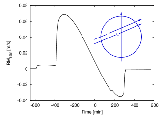
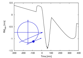
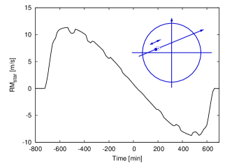
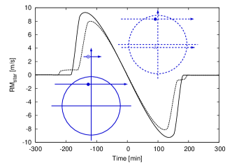
Figure 2: Four examples of the Rossiter-McLaughlin effect with different transit geometries. Each panel shows the effects of the moon superimposed on the RM curve and the system configuration during the transit. The big circle with axis, the big spot and the dot in the small circle represent the star, the planet and the moon, respectively. The illustrations are to scale.

We developed a new algorithm for precise calculations of arbitrary transiting systems with a satellite. The observed quantities are the light curve and the Rossiter-McLaughlin curve. The masses, radii, orbital periods, inclinations and ascending nodes of the planet and the satellite are input parameters. The orbital phase of the satellite at mid-transit is also adjustable. The dynamical evolution of such a system is given by a three-body problem. At this point, we included an approximation where the planet and the satellite orbit around their barycentre and this barycentre orbits the star with uniform velocity. To exclude the short-time escape of the moon, the system had to fulfil the criterion on the Hill sphere and must orbit at larger radius than the Roche limit (Szabó et al. 2006).

The star is parametrized by its mass and limb darkening (Phoenix linear limb darkening coefficients are default, Claret 2000). Stellar radius is calculated from the mass using the models of the Padova isochrones with solar metalicity (Girardi et al. 2002). The apparent brightness and the radial velocity of the star change while the satellite transits. These observables are calculated by integrating over a simulated and discretized stellar disk. Where the planet and the satellite hide the stellar surface, pixels get zero weight. We use a model star with a radius of 1000 pixels. The pixels are rectangular, and each has two values: (i) local surface brightness and (ii) local velocity of the surface element, calculated from the radius, the stellar spin period and the position of the pixel.

The radii of orbits (planet and satellite) are calculated from the orbital periods, according to Kepler’s third law. The velocity vectors of the planet and the moon are derived from their position vectors and their orbital periods. These determine the radial velocity of the barycentre of the star via the criterion of the conservation of momentum, leading to a simple dynamical dumbbell-model.

This algorithm is implemented in a user-friendly GUI interface with four animated simulation windows in a shared Front Panel. They show (i) a distant view of the orbit of the planet and the satellite; (ii) a zoom into the transit geometry; (iii) the surface of the star with the transiting objects and (iv) the light curves and RM curves. The input parameters, stability information and applied time step are indicated in the parameter panel (main window, Simon et al. 2009).

The user can set the time step and can select real time or background calculations. It is also possible to generate a large number of of photometric and RM curves using system parameters randomly within a given interval. The output files contain a detailed file header with the system data and three columns with values of time, magnitude and radial velocity data.

2.1 Sample simulations

We simulated many systems with various parameters, and identified different transit scenarios that lead to morphologically different light curves and Rossiter-McLaughlin curves. This will lead to a classification of transit geometries from an observational point of view. First we simulated the two most prominent examples in our Solar System: the transit of Earth with the Moon, and the transit of the Jupiter with Ganymede. The light curve and RM curves are presented in the upper panels of Fig. 1. We concluded that the photometric effects of these moons are too little for a direct detection: they are in the order of 5–10 ppm. This is an order of magnitude less than the photometric accuracy of the Kepler space telescope (255 ppm $rms$ in the time series of 115 quiet stars in Short Cadence data, Gilliand et al. 2010). The RM effect due to the moon is again very small, 1 cm/s and 4 cm/s, respectively. These velocity deviations are beyond the current technology and also are also much smaller than the intrinsic stellar noise for a wide range of stellar parameters (cf. Sect. 4). For these configurations, the only chance for the detection is the Photocentric Transit Timing Variation (Szabó et al. 2006, Simon et al. 2007). If the moon is so close that during one transit it orbits the planet more than once, this can lead to marked waves (wobbling) in the RM curve (Fig. 2 lower panels) that can have an amplitude of 10–100 cm/s.

The lower panels of Fig. 1 show systems where the detection is more promising. We designed systems with a little star, and very large, Earth-sized moons of transiting Saturn-like planets. The data of the systems is summarized in Table 1. Here the effects of the moon can be as large as 730 ppm in photometry, or 80 cm/s in radial velocity. Both values are promising, so the conclusion is that if such systems exist, they could be discovered with the present techniques. In these particular examples the moons orbit very close to the planet, mutual planet-satellite eclipses occur, but the presence of mutual eclipses is not a necessary criterion for a successful discovery. The most important parameter is the size of the moon, that must be in the order of the size of the Earth. This is the size that can cause directly observable effects, almost regardless of the orbital period of the satellite itself.

Table 2: Transit classification and proposed methods for detecting the moon. LC: direct detection in the light curves, TTV_b and TTV_p: barycentric and photocentric TTV, TDV: Transit Duration Variation, RM: the Rossiter-McLaughlin effect, RM(TV): Transit Timing Variation of the RM effect.

	Static	Slow	Rapid
	moon	moon	moon
Full	LC, TTVb,	LC, TTVb,	LC (wobbling),
Transit	TTVp, RM	TTVp, TDV	RM (wobbling)
		RM
Tangent
planet	LC, RM	LC, RM	LC, RM
Planet	TTVb,	TTVb, TDV	TTVb, TDV,
only	RM(TV)	RM	RM

2.2 Classification of transit scenarios

By now, there are several methods that offer the detection of exomoons, while they are not equivalently effective for different transit configurations. A possible classification scheme for transits is proposed here from the point of view of the applicable methods.

We have run many transits with the purpose of mapping the entire parameter space. These lead to different morphology of light curve and RM curve, therefore different methods are required to detect the moon itself in the measurements.

There are three distinctly different geometrical configurations which we call as the “static” moon, the “slow” moon and the “rapid” moon. A “static” moon means that it has a very long orbital period, comparable to that of the planet itself. In a such configuration, the relative position of the moon to the planet does not change significantly during one transit. Thus, one transit of the planet and one transit of the moon, superimposed to each other, are observed. The shape of the light curves and RM curves are the same for the planet and the moon, but time-lagged because of the geometry (upper left panel in Fig. 2). In extreme cases, e.g. when the semi-major axis of the moon is greater than the stellar diameter, the planet may complete the entire transit before the moon contacts the stellar disk, in which case we observe totally distinct “planet” and “moon” transits – the latter with a much smaller depth.

In the case of a “slow” moon, a difference can be detected between the duration of the transit of the moon and that of the planet, due to the slowly changing relative position during the event. This is favourable because the orbital period can also be estimated from one single transit observation (cf. Sect. 4).

In the two cases described above there are some scenarios when only the planet or the moon transits completely, resulting in a short grazing eclipse of the stellar disk by the planet or the moon (“tangent planet” configuration, see in Fig. 2, top right). There is another setup when the moon does not transit at all, but causes TTV and TDV in the transit of the planet. The lower right panel in Fig. 2 shows two such transits with the moon on the opposite sides of the planet.

In the third case the satellite orbits rapidly, which produces a characteristic wobbling in the light curves and the RM curves. The great variety of such extreme geometries is interesting but the large diversity of possible scenarios does not enable drawing a consistent picture (see Fig. 2, bottom left, for an example).

These configurations prominently differ and give different observable effects. In Table 2 we summarise all the cases, together with the methods that can be applied to detect the satellite. In the following we restrict the discussion to the slow and static moons.

3 Inversion of the Rossiter-McLaughlin effect

The task of analysing real observations is to recognize the presence of an exomoon if it exists, and to estimate its parameters and parameter errors. Here we present an elaborated analysis of parameter reconstruction, correlations and degeneracies from noisy simulated observations utilising bounded error analysis. The transiting model system consists of a Uranus-sized planet with one large, Earth-sized moon around a 0.8 M_⊙ mass star (see data of Simulation 5). The RM curve has been equidistantly sampled in 3 minute stepsize and then noisified with various amount (20, 50, 100 cm/s) of uniform noise. While the RM effect of the moon itself had 1 m/s amplitude, these refer to approximate signal (of the moon) - to -noise ratios of 5, 2 and 1, respectively.

It is worth noting that we do not claim that the RM effect is efficient enough for discovering exomoons. Our aim here is to understand which parameters can be extracted from RM observations, regardless of to what extent they can be constrained from transit photometry.

A joint analysis of the RM effect and transit photometry is beyond the scope of the present paper and will be discussed in a forthcoming publication.

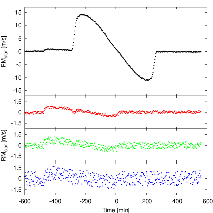
Figure 3: A simulated observation (top panel) and the residuals after fitting a single planet solution (bottom panels). The latter plots correspond to the S/N=5, 2 and 1 levels.

3.1 Parameter reconstruction

Let $P$ and $M$ denote the real parameter vectors of the planet and the moon, respectively, which are to be estimated from the observations. For this we need to locate the parameter vectors of the planet, $\tilde{P}_{i}$ and the moon, $\tilde{M}_{i}$ that tune the simulator into a good agreement with the observed data. Let $v_{r,sim}$ mean the template RM curves (they are not noisy), and $v_{r,obs}$ be the observed data (simulated observations), which are noisy. The best-fit parameters of the planet, $\mathcal{P}$ have been determined by minimising the $rms$ scatter of the residuals between observations and templates containing a single planet only:

$$\mathcal{P}=\arg\min_{\tilde{P}_{i}}\left[\sum\left(v_{r,obs}-v_{r,sim,\tilde{P_{i}}}\right)^{2}\right].$$ (1)

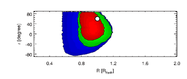
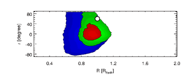
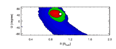
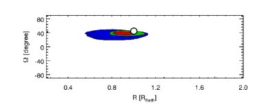
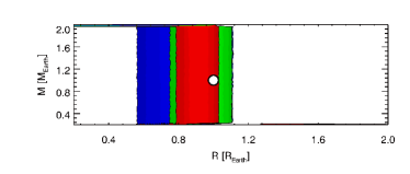
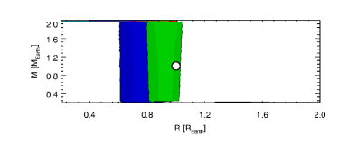
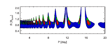
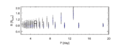
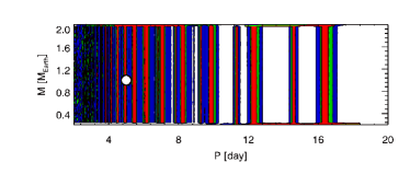
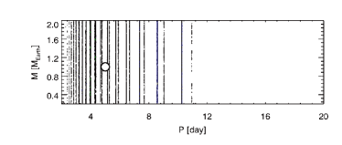
Figure 4: Joint confidence intervals of the moon parameters around the exact solution. The differences between the left and the right columns demonstrate how the parameter reconstruction improves when using moon transit photometry, i.e. the central transit time of the moon is known (plots in the right columns). Different colours show fittings with different S/N ratios (red: S/N=5, green: S/N=2, blue: S/N=1), while the large open circles represent the input parameters of the simulated observations. See Table 1 for the meaning of the parameters.

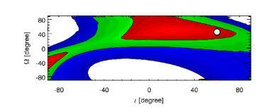
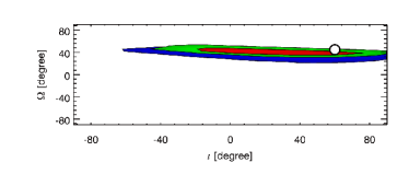
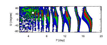
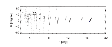
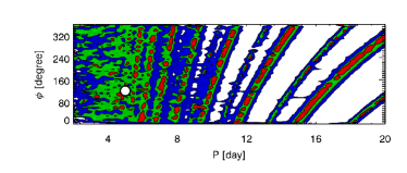
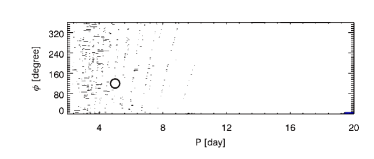
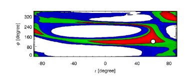
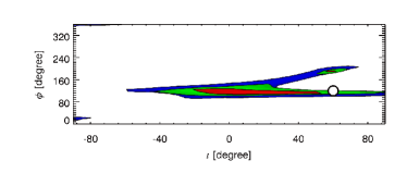
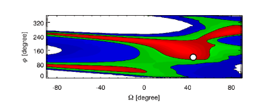
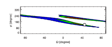
Figure 5: The continuation of Fig. 4. Here $\phi$ means the orbital phase of the moon around the planet.

We determine $\mathcal{M}$, the parameter vector of the moon in the second step. The residuals between the observations and the planet template contain the signal from the moon and noise. We fit this residual with tuning the parameters of the moon:

$$\mathcal{M}=\arg\min_{\tilde{M}_{i}}\left[\sum\left(v_{r,obs}-v_{r,sim,\mathcal{P}}-v_{r,sim,\mathcal{P},\tilde{M_{i}}}\right)^{2}\right].$$ (2)

In this formulation we decoupled the parameter estimation of the planet and that of the moon. Our tests have proven that this can be done. This is because the RM signal of the moon is only a slight perturbation in the RM pattern of the planet. Thus, the planet parameters can be reconstructed accurately enough that they do not influence the selection of the appropriate moon model in the second step.

3.2 Error analysis

After determining the parameters of the star and the planet, there remain 6 independent parameters of the moon. The confidence region in this 6-dimensional hyperspace has been mapped in 2-dimensional plane sections that the 15 possible parameter-parameter pairs span. $A_{x1,x2}$ is the joint confidence region (region of acceptance) of $x_{1}$ and $x_{2}$ in the $X=x_{1},x_{2},...$ hyperspace if

$$\int_{A_{x1,x2}}P\big{(}$\rm$obs\ \big{|}X)\ \ {\rm d}X=C,$$ (3)

where $obs$ means the observed data set with errors, and $C$ is the level of confidence. The smallest confidence interval at a given $C$ confidence is conjured by a certain likelihood value that can be determined experimentally. The $P()$ probabilities are calculated from the reduced standard deviations of the fits, using $\chi^{2}$ statistics. With this definition of the confidence interval the correlations can be recognized easily, because correlated parameters depend a lot on each other in the region of acceptance. A parameter that can be well reconstructed must have small confidence interval in all sections, and must not be strongly correlated to other parameters.

We have run a large number of models in the parameter space. First, we fitted a single-planet model to the simulated observations and minimized the residuals. In this step, we have run 1000 randomly simulated planet to map the structure of the grid, to estimate the minimum. Then we refined the grid locally and run $10^{4}$ planet templates. Among them, $\approx$ 10 possible planet solutions gave equivalently small residuals, ensuring that the grid was fine enough. The parameters of the best fitting planet were input parameters for modelling the moon.

In the second step, 1.5$\times 10^{6}$ transits were simulated with random initial geometries of the satellite. The templates were allowed to shift in time while fitting to the simulated observations. These resulted in 2.7$\times 10^{9}$ fittings altogether.

The likelihood limit defining the 95% confidence region has been deduced from the surface of $rms$ scatter experimentally. For this, 1000 bootstrap observations were calculated using the exact system parameters, noisified with different realizations of the same simulated observational noise. Then we determined the best-fit model planet, and calculated the residuals to the $M$ (simulation input) moon model. We mapped the 95% acceptance regions of parameters, therefore the $rms$ scatter limit was set to include 95% of these deviations. The resulting limits were $rms$ scatter of 0.149 m/s, 0.313 m/s and 0.609 m/s for the simulated observations of S/N=5, 2, 1 quality, respectively. These are, of course, particularly optimistic scenarios.

4 Discussion

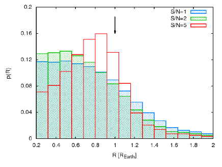
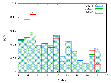
Figure 6: Posterior probability distributions of $R$ and $P$, marginalized from the fit likelihoods in the $P$–$R$ subspace with uniform priors. The three different distributions refer to S/N levels of 1, 2 and 5 with the same colour coding as in Figs. 3–4–5. The arrow shows the input value of the moon parameters.

The joint confidence intervals of the parameter pairs are shown in 20 panels in Figs. 4 and 5. Fig. 4 shows sections where the plotted parameters promise a reliable reconstruction. The best results are given for the size of the moon, that is closely linked to the amplitude of the residuals in the RM curve, after subtracting the best-fit planet. The radius is well reproduced in all sections and did not suffer serious degenerations. The topmost row suggests that the size is a little biased and the inclination of the moon is essentially unknown. This is because the residuals of the planet fitting is forced to be close to zero, consequently the size of the moon is slightly underestimated. For this smaller moon, a lower inclination parameter is preferred.

The ascending node of the orbit is somewhat correlated with the radius. Interestingly, once other parameters are well constrained, $\Omega$ can be determined very accurately as Fig. 4 shows (see the right panel in the second row). The 3rd and 5th rows of Fig. 4 demonstrate that there is no information on the mass of the satellite from the analysis of radial velocity, all probed masses are equally probable. The most important conclusion is that the mass of the satellite must be omitted from the analysis, i.e. a fixed value for the mass or a fixed assumption on the density of the satellite will lead to equally reliable solutions in the other parameters with a much faster process. The abscissa of the 4th and 5th panels in Fig. 4 show the orbital period of the moon. Surprisingly, there is some information in the light curve for this period, as values between 2–10 days are preferred (the model moon has 5 days period). Because of the little position change of the moon during the transit, the residual RM effect due to the moon will last a somewhat shorter or longer time than that of the planet, which may be detected.

Fig. 5 shows further sections where degenerations are prominent. The joint confidence intervals evidently show that the angle parameters, $\iota$, $\phi$ and $\Omega$ are seriously interrelated. Acceptable solutions can be characterized with very different values of $\Omega$ or $\phi$, because the orbital period of the moon is unknown (see the 2nd and 3rd rows). The 4th row shows that $\iota$ data do not constrain $\phi$ well. We suggest that a reliable value for $\iota$ will have to be assumed in practical applications, and the other two angle parameters should be taken out of fitting (they can be either marginalized or evaluated along some prior with Bayesian analysis).

However, these limitations of parameter determination do not lessen dramatically the power of radial velocity analysis in the exploration of exomoons. This method nicely completes the evaluation of photometry, since the mass can be determined from (barycentric) TTV. Simon et al. (2007) showed that from photocentric TTV_p we get some information on the radius of the satellite, but this is correlated with the density of the moon. The analysis of RM effects give prior information on the size of the moon, and the combination of all methods, theoretically, may lead to the direct experimental determination of the density of the exomoons.

In Fig. 6, we show the posterior probability distributions of $P$ and $R$, marginalized from the likelihood data with assuming uniform priors to all variables. The reconstruction of $R$ is satisfactory, although the radius is somewhat biased toward smaller sizes. There is some information for the period, too, which is somewhat surprising as the orbital period of the moon is $\approx 1/12$ transit duration. The increasing noise level does not bias the mode of the distributions, but gives the wings slightly more weight.

4.1 The general case of main sequence dwarf stars

We have shown the reconstruction of parameters for a 0.8 M_⊙ main-sequence star, which has a spectral type of K0 in case of solar metallicity. It is very important to note that our results are general and indicative for other types of stars. Although the signal will be smaller for bigger stars, the shape of the curves do not change significantly, hence error propagation will follow the same scenario as presented in Figs. 4-5. Consequently, the general behaviour of the parameters concerning their stability and degenerations will be the same. For a general case, we propose that the moon’s radius is the best parameter for reconstruction; in some cases, the orbital period might be also constrained.

Earlier type stars have larger radius, hence the area eclipsed by the moon is a smaller fraction of the projected stellar disk. The other parameter that determines the $A_{RM}$ half-amplitude of the RM effect is the $v_{rot}\sin i$ rotation velocity of the star, such that

$$A_{RM}\ \propto\ {\left(R\over R_{*}\right)^{2}}\ v_{rot}\sin i,$$ (4)

where $R$ denotes the radius of the moon, $R_{*}$ is the stellar radius and we can assume that $\sin i\approx 1$ for those systems that display transits and RM effect. Equality is true in Eq. 4 if we neglect limb darkening. Limb darkening can reduce the amplitude of the RM effect by 20–40%, depending on the exact intensity profile of the stellar disk. We can combine the RM effect of a moon and a planet together,

$$A_{RM,m+p}\propto{R_{p}^{2}+R^{2}\over R_{*}^{2}}\ v_{rot}.$$ (5)

Now an upper estimate can be given for the size of the moon if it is not detected in the residuals of the RM curve. In this case the RM effect of the moon is hidden in the scatter of the radial velocity data, i.e. $3\sigma_{v_{rad}}$ is larger than the satellite’s effect:

$$3\sigma_{v_{rad}}>A_{RM}={R^{2}\over R_{*}^{2}}v_{rot}.$$ (6)

Rearranging this for the size of the moon, the upper limit is given as $R<\sqrt{3\sigma_{v_{rad}}/v_{rot}}R_{*}$, or simply substituting the amplitude of the measured RM effect (and assuming $A_{RM,m+p}\approx A_{RM,planet}=R_{p}^{2}/R_{*}^{2}v_{rot}$),

$$R<\sqrt{3\sigma_{v_{rad}}\over A_{RM,planet}}R_{p}.$$ (7)

The confidence of this estimate is 99.9 %, i.e. $3\sigma$ confidence.

Which spectral types represent the best candidates for a successful detection of exomoons with the RM effect? To answer this question, we performed simple calculations for stars in the Pleiades open cluster, assuming that every star has a planet with a Ganymede-sized moon in central transit. Our intention was to predict the amplitude of the satellite’s RM effect (assumed to be independent of that of the planet), as a function of stellar mass.

The $B-V$ colours and $v\sin i$ data for Pleiades stars were taken from Queloz et al. (1998). Stellar masses and radii were estimated from the $B-V$ colour, using the latest Padova isochrones (Bertelli et al. 2008), adopting 70 Myr for the age and Z=0.017 for the metallicity (Boesgaard & Friel 1990). We calculated the amplitude of the RM effect according to Eq. 4, inserting the stellar radius and rotation velocity for each star, and substituting the size of Ganymede. The results are plotted in Fig. 7 with open circles.

Although there are hints of a tendency, the scatter is large, which can be explained by the different spin axis orientations and different rotation evolution for each star. The shape of the distribution in Fig. 7 can be better seen using a statistical relationship for the rotation period of main-sequence stars determined by Barnes (2007): $P_{rot}\propto(B-V-0.4)^{0.601}t^{0.52}\$ days, where $t$ is the age of the star. This formula is singular at $B-V=0.4$, thus it is valid for stars later than F5, approximately. Similarly to the individual stars, the $B-V$ colours of the isochrone points have been converted to masses and radii. The rotation velocity has then been calculated as $v_{rot}=2\pi R_{*}/P$ (we kept assuming $\sin i\approx 1$). To estimate RM amplitudes, we again used Eq. 4 and the size of Ganymede. In Fig. 7, the solid line shows the resulting average RM amplitude. We conclude that stars below 0.6–0.8 M_⊙ offer the best opportunity to detect the RM effect of the exomoons. Stars with masses greater than 1.2 M_⊙ do also show larger effect, however, stellar variability quickly becomes dominant with the increasing mass.

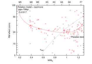
Figure 7: Half amplitude of the Rossiter-McLaughlin effect due to Ganymede-sized moons of planets orbiting G, K and M dwarfs. Solid line: empirical model based on Barnes (2007) rotation model and isochrones. Open circles: individual stars of the Pleiades. The dashed curve shows the amplitude of solar-like oscillations.

This variability has two dominant components: the jitter due to convective motions (including the convectively excited solar-like oscillations) and the rotational modulation due to stellar activity. Among the brighter dwarf stars, old, inactive G and K dwarfs offer the best performance: a few stars are known to have $<$1 m/s jitter, while they typically have jitter levels in the 1–5 m/s regime (Saar et al. 2003, Wright 2005, O’Toole et al. 2008). On the contrary, some F-type stars display large jitter that even challenges asteroseismology (see the example of Procyon in Arentoft et al. 2008) and the detection of long-period planets (Lagrange et al. 2009). The jitter from solar-like oscillations can be estimated via the scaling relation of the velocity amplitude, which depends on the light-to-mass ratio of the star:

$$v_{osc}={L/L_{\odot}\over M/M_{\odot}}\left(23.4\pm 1.4\right)\ \ {\rm cm/s}$$ (8)

(Kjeldsen & Bedding 1995). The predicted oscillation velocity amplitudes are also plotted in Fig. 7 with the dashed line (blue in colour). Since M-dwarf stars have very small $L/M$ ratio, and consequently the amplitude of solar-like oscillations is tiny, they are promising candidates to be quested for exomoons. These stars are faint in the visual, but recent work of Bean et al. (2009), for example, has opened the door to the sub-m/s velocimetric accuracy in the infrared with CRIRES on VLT.

It is worth noting that late M-dwarfs (beyond M4) exhibit larger rotation velocities (Jenkins et al. 2009), which makes them difficult targets for high-precision RV measurements because rapid rotation washes out the spectral features (Bouchy et al. 2001). Hence, the best targets for exomoon exploration are the K and early M dwarf stars, for which both rotation and activity reach a minimum level (Jenkins et al. 2009, Wright 2005).

In case of higher stellar activity, the situation is not entirely hopeless, as illustrated by a recent study by Queloz et al. (2009), who filtered out activity with a Fourier polynomial using the first rotation harmonics. This way they pushed the residuals from $\pm 20$ m/s to $\pm$ 5 m/s. Similar residual levels in fitting the RM effect were reached by Triaud et al. (2009).

It is known that the frequency of giant planets increases linearly with the parent-star mass for stars between 0.4 and 3 $M_{\odot}$ (Ida & Lin 2005, Kennedy & Kenyon 2008), with e.g., 6$\%$ frequency of giant planets around 1 $M_{\odot}$ and 10$\%$ frequency around 1.5 $M_{\odot}$. However, we know planets around red dwarfs and there is observational indication for a few multiple planetary systems among them (e.g. Rivera et al. 2005). The possible detection of exomoons around planets of larger stars, if these satellites ever exist, is a significant challenge for signal processing to minimise the ambiguity caused by the higher level of velocity jitter.

A more elaborated distinction between signals of exoplanets and signals from stellar physics requires a deep analysis that is beyond the scope of this paper. There is reason for some optimism because the time-scales of the exoplanet-exomoon systems and that of the stellar signals are usually very different. Moreover, rapid development in instrumentation may reach levels of precision that were unimaginable even a few years ago.

References

- [1] Agol, E., Steffen, J., Sari, R., Clarkson, W. 2005, MNRAS, 359, 567
- [2] Arentoft, T. et al. 2008, ApJ, 687, 1180
- [3] Asimov, I. 1979, Extraterrestrial civilizations, Crown Publishers, NY
- [4] Barnes, S. A. 2007, ApJ, 669, 1167
- [5] Bean, J. L. et al. 2009, ApJ, submitted (arXiv: 0911.3148)
- [6] Bertelli, G. et al. 2008, A&A, 484, 815
- [7] Boesgaard, A. N., Friel, E., D. 1990, ApJ, 351, 467
- [8] Bouchy, F., Pepe, F. & Queloz, D. 2001 A&A, 374, 733
- [9] Claret, A. 2000, A&A, 363, 1081
- [10] Díaz, R. F. et al. 2008, ApJ, 682, 49
- [11] Drilling, J. S., Landolt, A. U., Cox, N (ed.) 2000, in: Astrophysical Quantities, Springer-Verlag, 381
- [12] Gaudi, B. S., Winn, J. N. 2007, ApJ, 655, 550
- [13] Gilliand, R. L. et al. 2010, ApJ, in press (arXiv: 1001.0142)
- [14] Girardi, L., Bertelli, A., Bressan, C. et al. 2002, A&A, 391, 195
- [15] Ida, S., Lin, D. N. C. 2005, ApJ, 626, 1045
- [16] Jenkins, J. S. et al. 2009, ApJ, 704, 975
- [17] Kennedy, G. M., Kenyon, S. J. 2008, ApJ, 673, 502
- [18] Kipping, D. M. 2008, MNRAS, 389, 1383
- [19] Kipping, D. M. 2009, MNRAS, 396, 1797
- [20] Kipping, D. M., Fossey, S., J., Campanella, G. 2009, MNRAS, 400, 398
- [21] Kjeldsen, H., Bedding, T. R. 1995, A&A, 293, 87
- [22] Mayor, M. 1998, A&A, 335, 183
- [23] Mayor, M. et al. 2009, A&A, 507, 487
- [24] Lagrange, A-M. et al. 2009, A&A, 495, 335
- [25] Lewis, K. M., Sackett, P. D., Mardling, R. A. 2008, ApJ, 685, L153
- [26] Li, C.-H. et al. 2008, Nature, 452, 610
- [27] Liebig, C. and Wambsganss, J. 2009, A&A, submitted (arXiv: 0912.2076)
- [28] O’Toole, S. J. et al. 2008, MNRAS, 386, 516
- [29] Pál, A., Kocsis, B. 2008, MNRAS, 389, 191
- [30] Queloz, D., Allain, S., Mermilliod, J.-C., Bouvier, J., Major, M. 1998 A&A, 335, 183
- [31] Queloz, D. et al. 2009, A&A, 506, 303
- [32] Rivera, E. J. et al. 2005, ApJ, 634, 625
- [33] Saar, S. H. et al. 2003, The Future of Cool-Star Astrophysics: 12th Cambridge Workshop on Cool Stars, (eds. A. Brown, G.M. Harper, and T.R. Ayres), University of Colorado, 694
- [34] Sartoretti, P., Schneider, J. 1999, A&AS, 134, 553
- [35] Simon, A. E., Szatmáry, K., Szabó, Gy. M. 2007, A&A, 470, 727
- [36] Simon, A. E., Szabó, Gy. M., Szatmáry, K. 2009, EM&P, 105, 385
- [37] Szabó, Gy. M., Szatmáry, K., Divéki, Zs., Simon, A. 2006, A&A, 450, 395
- [38] Triaud, A. H. M. J. et al. 2009, A&A, 506, 377
- [39] Wagner, N. 1936, Unveiling the universe, The Research publishers, Scranton, PA
- [40] Wright J. T. 2005, PASP, 117, 657