The chaotic set and the cross section for chaotic scattering in 3 degrees of freedom

Abstract

This article treats chaotic scattering with three degrees of freedom, where one of them is open and the other two are closed, as a first step toward a more general understanding of chaotic scattering in higher dimensions. Despite of the strong restrictions it breaks the essential simplicity implicit in any two-dimensional time-independent scattering problem. Introducing the third degree of freedom by breaking a continuous symmetry, we first explore the topological structure of the homoclinic/heteroclinic tangle and the structures in the scattering functions. Then we work out implications of these structures for the doubly differential cross section. The most prominent structures in the cross section are rainbow singularities. They form a fractal pattern which reflects the fractal structure of the chaotic invariant set. This allows to determine structures in the cross section from the invariant set and conversely, to obtain information about the topology of the invariant set from the cross section. The latter is a contribution to the inverse scattering problem for chaotic systems.

¹ Instituto de Ciencias Físicas
Universidad Nacional Autónoma de México,
Av. Universidad s/n, Apdo. Postal 48-3 Cuernavaca, Morelos, México.
² Zurich University of Applied Sciences
Institute of Applied Simulation
Grüental, P.O. Box
CH-8820 Waedenswil, Schweiz.
³ Centro Internacional de Ciencias AC
Apartado Postal 6-101
C.P. 62131 Cuernavaca, Morelos, México.

karelz@fis.unam.mx

PACS Numbers 05 45

1 Introduction

Chaotic scattering with two degrees of freedom is fairly well understood [1, 2, 3, 4, 5, 6] both for hard chaos (hyperbolicity) and soft chaos in terms of Smale’s horseshoe construct [7, 8]. In a time-independent Hamiltonian system with two degrees of freedom, Smale’s horseshoe displays the invariant manifolds which qualitatively separate the dynamics. On an appropriate surface of section these invariant sets become smooth curves. This has two advantages:1) we can study objects easily if they can be drawn on paper, and 2) they separate the phase space dynamics if they close or go to infinity in both directions.

Scattering functions [8, 9, 10] and cross sections [11, 12] have been analysed both statistically and geometrically, and the inverse scattering problem has been tackled [9, 13] (for general background information see the text books [14, 15, 16]).

Now the effort must be directed towards higher dimensional systems, as they are relevant in astrophysics [17, 18] or chemistry [19, 20, 21]. How do we proceed to generalise this success in the description of chaotic scattering to more than two degrees of freedom? There are previous important steps particularly by Wiggins [22, 23, 24], but also by Ott [25]. The former develops a formal theory that is difficult to apply but gives important foundations of the problem. The latter show, that a straight forward generalisation of the three-disc system in triangular configuration to a four sphere problem in tetrahedral configuration is feasible, but the invariant manifolds are low dimensional and thus not relevant so some physical problems, as they are difficult to detect. We have suggested in an earlier paper that it can be useful to have a gradual approach to a change in dimension by breaking a continuous symmetry of the problem [26].

In the present paper we shall follow this last suggestion and apply it to the simplest possible three degrees of freedom configuration, with two bound and only one open degree of freedom. Despite of this strong restriction, we are now definitely beyond the situation, where Smale’s theory can be used, and systems of that kind are not without interest. We might consider guiding channels with one open degree of freedom, or we can consider equivalently three interacting particles in one dimension, under conditions where asymptotically one pair must always be bound.

We shall focus on the topological structure of the invariant set rather than on details of trajectories, because the former properties tend to be generic , i.e. robust and embody the most relevant information about the chaotic system [13]. We are thus looking for some generalisation of the horseshoe to higher dimensions. A simple minded generalisation does not exist, as can be seen from the work of Wiggins [23]. The basic reason is that the dimension of the invariants manifolds of hyperbolic points is too low.

We proceed by analysing the transition from a system, which has an ${\cal O}(2)$ symmetry group in the three dimensional position space, reducing the problem for a fixed value of the angular momentum to a system with two degrees of freedom. We shall then introduce in the reaction region (i.e. in the region where the asymptotic Hamiltonian is not valid) a symmetry breaking term. This will allow us to start our analysis with a continuous stack of horseshoes corresponding to different values of the angular momentum and observe how the structure evolves as the invariance breaks down. We then study the implications for scattering functions and for the doubly differential cross sections. The fractal structure of singularities in the latter, i. e. the rainbow structures, is directly related to the structure of the chaotic set, leading to an additional important contribution to the corresponding inverse scattering problem. Indeed we shall also see, that the basic idea developed is not limited to three degrees of freedom nor to one open degree of freedom, but these aspects will only be commented.

We shall illustrate our procedures with three examples. First a channel with harmonic walls in two directions that deforms to some more complicated potential in some compact region of configuration space. This is equivalent to two pairs of particles bound by harmonic forces and interacting between each other weakly. The second is a bottle shaped billiard that is either connected to a channel billiard or has an opening that separates the interior from the exterior in some plane in configuration space. Finally for numerical convenience we shall use a $\delta$ kicked system of two degrees of freedom, which is topologically equivalent to the Poincaré maps of the first system.

As far as the physical implications are concerned, it does not seem easy to emulate systems with such restrictions and no significant friction, though it might become feasible with Bose Einstein condensates at some point in the future. The alternatives in celestial mechanics imply higher dimensions and/or more complicated asymptotes, as is the case with the breaking of the Jacobi invariant in ref [26]. Yet the results are certainly useful for semi-classical considerations, such as e.g. the ones used in [27] to design and interpret a microwave experiment.

The paper is structured as follows: in the next section we shall define the class of three degree of freedom systems, which we shall consider as well as the specific examples we shall use. Next we proceed to construct the invariant sets and study them as a function of the symmetry breaking. In section four we derive the scattering functions, that is the behaviour of outgoing asymptotes as a function of the incoming ones. This will allow us to discuss the rainbow effects in the doubly differential cross sections in section five. We finally proceed to comment on the scope of our results as well as implications for semi-classics.

2 The class of systems considered and the model systems

We consider a scattering system with three degrees of freedom where one of them is open and the other two are closed. We imagine that the first degree of freedom is a translational degree of freedom between projectile and target, the second degree of freedom is a vibrational degree of freedom and the third one is a rotational degree of freedom.

The first particular model system of this class which we use is a rotationally symmetric channel containing an additional short range potential representing some obstacle (the target) sitting in the otherwise empty channel. Accordingly the total Hamiltonian of the system splits, as always in scattering systems, in a free Hamiltonian $H_{0}$ describing the asymptotic free motion ( in this particular case it is the motion in the empty channel), and an additional interaction $W$ which is the short range scattering potential, i.e.

$$H=H_{0}+W$$ (1)

We imagine that the channel runs straight in one direction and we use the coordinate $q$ along the channel, $p$ is the momentum conjugate to $q$. In the transverse direction the motion of the projectile is confined by the channel and we assume that the potential which represents the walls of the channel is quadratic in the transverse coordinates. Because of the rotational symmetry of the empty channel one natural choice is to use cylindrical coordinates $\rho$ and $\theta$ and their conjugate momenta $p_{\rho}$ and $L$ and also to include into the free Hamiltonian the quadratic potential and the transverse kinetic energy in these coordinates. Since the radial motion is an oscillation, it is sometimes more convenient to use action and angle variables $I$ and $\phi$ for the radial degree of freedom. We will switch freely between these two possibilities according to which one is more convenient at the moment. The asymptotic Hamiltonian written in cylindrical position and momentum coordinates results as

$$H_{0}=p^{2}/2+p_{\rho}^{2}/2+L^{2}/(2\rho^{2})+\rho^{2}/2$$ (2)

We choose units of time such that the transverse oscillation frequency in the empty channel is one. To describe the obstacle we use later as model of demonstration the potential

$$W=-\frac{\exp(-D)}{D}$$ (3)

where

$$D^{2}=q^{2}+\rho^{2}(\sin^{2}\theta+(1+A)^{2}\cos^{2}\theta)+1$$ (4)

The extra constant, taken as one, avoids singularities in the potential. Very important for the following is the parameter $A$ which measures the deviation of the interaction potential from rotational symmetry. For $A=0$ we have perfect symmetry and since the free Hamiltonian $H_{0}$ is also symmetric, the total system is symmetric, the angular momentum $L$ is conserved and the system can be reduced to two degrees of freedom. For the value $L=0$ the symmetric system reduces to the one used in [11]. This reference also contains a physical interpretation of similar potential models.

Next we need labels for the asymptotes of the system, i.e. the trajectories of the free motion described by $H_{0}$. The optimal possibility is to use 5 independent quantities which all are constant along the asymptotic trajectories. Since in any Hamiltonian system the energy $E$ is conserved, both under the free asymptotic dynamics and under the full dynamics, we use $E$ as one of these labels. Asymptotically the translational degree of freedom decouples from the other ones and the momentum $p$ becomes constant. We use $p$ as second asymptotic variable. The sign of $p$ indicates into which direction the asymptotic motion runs and therefore a comparison between the signs of initial and final $p$ distinguishes transmission and reflection. In addition, since $H_{0}$ is independent of $\theta$, the conjugate variable $L$ is conserved under the asymptotic dynamics and it is convenient to use it as third label for asymptotic trajectories. To distinguish the various asymptotic trajectories with the same values of $E$, $p$ and $L$ we need two additional labels giving the relative phase shifts between the translational motion along the channel and the other two motions. The systematic choice for these relative angles are the reduced phases constructed along the following idea. In action variables we find for our particular system

$$H_{0}(p,I,L)=p^{2}/2+2I+|L|$$ (5)

Then the asymptotic equations of motion for $\phi$ and $\theta$ are

$$\frac{d\phi}{dt}=\frac{\partial H_{0}}{\partial I}=\omega_{\phi}(I,L)=2$$ (6)

$$\frac{d\theta}{dt}=\frac{\partial H_{0}}{\partial L}=\omega_{\theta}(I,L)=\pm 1$$ (7)

The sign appearing in equation 7 is the sign of the angular momentum. We define the reduced angles $\psi$ and $\chi$ belonging to $\theta$ and $\phi$ respectively as

$$\psi=\theta-\omega_{\theta}(I,L)q/p=\theta\mp q/p$$ (8)

$$\chi=\phi-\omega_{\phi}(I,L)q/p=\phi-2q/p$$ (9)

The sign in equation 8 is minus the sign of the angular momentum. A short calculation shows that these two reduced angles are constant under the asymptotic dynamics.

An equivalent possibility is the following: We use the values of the two coordinates $\phi$ and $\theta$ at the moment when the absolute value of $q$ reaches some very large value (in the numerical examples, we use $\|q\|=8$). We call these two particular values which serve as asymptotic labels $\chi$ and $\psi$ again. We use the index $in$ for initial asymptotic conditions and the index $out$ for the labels of outgoing asymptotes.

Since it is simpler to handle iterated maps instead of flows, we will use Poincaré maps to represent the dynamics of the system and to explain many ideas (an elementary explanation of the concept of Poincaré maps is found in section 2.5 of [28]). For the channel problem an appropriate intersection condition for the Poincaré map is to take the maximum of the cylindrical radial coordinate $\rho$. This choice has the advantage to coincide with the choice made for a billiard model which we also use later. Almost all trajectories intersect this surface transversely an infinite number of times and asymptotically the return time to this surface becomes constant, note the constant value of $\omega_{\phi}(I,L)=2$ in equation 6. The only exceptions are trajectories with action $I=0$ which run along spirals of constant value of $\rho$ without any radial oscillations. In the domain of the map we use the canonical coordinates $q$, $p$, $\theta$, $L$.

An alternative version of the reduced angles $\psi$ and $\chi$ for the map is obtained as follows: For trajectories with the value p of the asymptotic longitudinal momentum select an interval of large absolute values of $|q|$, say the interval $[Q,Q+|p|]$ where $Q$ is sufficiently large to guarantee that the trajectory is already in the asymptotic region. Observe the trajectory of the map until it steps into this interval. For this point define $\chi=2\pi(|q|-Q)/|p|$ and for $\psi$ take the actual value of $\theta$ in this point. Note that the initial point and the final point of the selected $q$ interval can be identified for the purpose of asymptotic labelling since they describe the same trajectory (one is the image of the other point under the action of the map) and lead to the same value of the angle $\chi$ since multiples of $2\pi$ are irrelevant. Therefore this line of initial conditions has the topology of a circle. An analogous construction also works well for the Poincaré maps of other model systems.

The second model of demonstration used is a billiard model, it describes scattering in a bottle. The boundary of the bottle will be defined with the aid of the following functions:

$$f(q)=\begin{cases}1.4\sqrt{1-q^{2}},&\hbox{ for }q\leq 0\\ a_{0}q^{2.5}+a_{1}q^{2}+1.4,&\hbox{ otherwise.}\end{cases}$$ (10)

$$r(q,\theta)=1+A\cos(\theta)\cos(\frac{q\pi}{2q_{0}})^{2}$$ (11)

The boundary itself is given by

$$\rho(q,\theta)=r(q,\theta)f(q)$$ (12)

Two dimensional billiards with the border described by function 10 have been studied in [29] and a similar model in [30].

The values of the constants $a_{i}$ are chosen to give a smooth boundary and to lead to an unstable quasi periodic orbit in the plane $q=0$ so that there is a complete binary horseshoe for the reduced rotationally symmetric case for $L=0$. Convenient values turn out to be:

$$a_{0} =\frac{14}{25}(3.49)^{-1/4}$$ (13)

$$a_{1} =-0.7$$ (14)

$$q_{0} =(3.49)^{1/2}$$ (15)

Also this model has a parameter $A$ which gives the distance from rotational symmetry and again for $A=0$ we have perfect symmetry and the system can be reduced to one with two degrees of freedom.

The billiard dynamics is the usual one with elastic reflection on the wall and free motion in the inside. The energy is a constant and proportional to the square of the momentum. Therefore we can set the velocity $\|v\|=1$ without loss of generality. The Poincaré map of the bottle model is the usual Birkhoff map on the wall of the billiard (these are explained in [31]). We only use weak deformations of the bottle such that this map coincides with the intersection condition of maximal cylinder radius $\rho$. Accordingly we use in the domain of the map the same coordinates $q$, $p$, $\theta$ and $L$ as in the channel model.

The Birkhoff-Poincaré map of this system has a binary horseshoe instead of the ternary one of the other two examples, and it has a surface of no return at a finite value of $q$, which makes is qualitatively different. Nevertheless we will see that it belongs to the same class of systems.

Since it is a lot more convenient and faster to investigate maps instead of flows we construct as third model a closed form example of a map acting on the 4 dimensional domain with coordinates $q$, $p$, $\theta$ and $L$. This model is constructed in a way that it can serve as a prototype Poincaré map for the whole class of systems considered in this article. It is based on the usual scheme of kick and free flight. The generating function for the kick is:

$$G(q,\theta,\tilde{p},\tilde{L})=q\tilde{p}+\theta\tilde{L}+(L_{max}-\tilde{L})(1+Acos\theta)V(q),$$ (16)

with potential function

$$V(q)=-e^{-q^{2}}.$$ (17)

We define the force function on the $q$ coordinate as

$$F(q)=-dV/dq=-2qe^{-q^{2}}.$$ (18)

And the kick map is implicitly given by:

$$\tilde{q} =\frac{\partial G}{\partial\tilde{p}} p =\frac{\partial G}{\partial q}$$ (19)

$$\tilde{\theta} =\frac{\partial G}{\partial\tilde{L}} L =\frac{\partial G}{\partial\theta}.$$ (20)

To construct a complete step of the map, the particles will perform first half of the free flight:

$$q^{\prime} =q_{n}+p_{n}/2$$ (21)

$$\theta^{\prime} =\theta_{n}+L_{n}/2$$ (22)

$$p^{\prime} =p_{n}$$ (23)

$$L^{\prime} =L_{n}$$ (24)

Afterwards, we give this auxiliary coordinates the kick, given explicitly by the next set of equations:

$$q^{\prime\prime} =q^{\prime}$$ (25)

$$\theta^{\prime\prime} =\theta^{\prime}-(1+A\cos\theta^{\prime})V(q^{\prime})$$ (26)

$$p^{\prime\prime} =p^{\prime}+(L_{max}-L^{\prime})\frac{(1+A\cos\theta^{\prime})F(q^{\prime})}{1+AV(q^{\prime})\sin\theta^{\prime}}$$ (27)

$$L^{\prime\prime} =\frac{L^{\prime}+L_{max}AV(q^{\prime})\sin\theta^{\prime}}{AV(q)\sin\theta^{\prime}+1}$$ (28)

And finally half a free flight is applied again:

$$q_{n+1} =q^{\prime\prime}+p^{\prime\prime}/2$$ (29)

$$\theta_{n+1} =\theta^{\prime\prime}+L^{\prime\prime}/2$$ (30)

$$p_{n+1} =p^{\prime\prime}$$ (31)

$$L_{n+1} =L^{\prime\prime}$$ (32)

This concludes the action of the map. Every step is symplectic, and the map behaves qualitatively as the Poincaré map of the first example.

We use mainly the map model for the presentation and explanation of our ideas. Below we compare some results of this map with the results of the other two models in order to convince ourselves that the map results are representative.

3 The topological structure of the chaotic invariant set

Since the interaction potential of equation 3 or of equation 17 is negative, there are trajectories with negative energy yet arbitrarily close to zero, going out extremely far and returning. Therefore our first example system has no points without return. Its outermost periodic orbits lie at $q=\pm\infty$. They are trajectories oscillating transverse to the channel and rotating at constant value of $q$, where $q$ is arbitrarily far away. Since any displacement of $q$ leads to an equivalent transverse oscillation, these transverse trajectories come in a whole continuum of copies. In the Poincaré map they lead to fixed points at $q=\pm\infty$, $p=0$ and these points are parabolic, i.e. neutrally stable in linear approximation. However the non-linearities of the map at finite values of $q$ make these points non linearly unstable and they have stable and unstable invariant manifolds. The stable manifolds consist of trajectories which go out to infinity monotonically, i.e. the absolute value of $q$ increases monotonically while at the same time the value of the momentum $p$ converges to zero. Asymptotically all energy of the motion goes to the transverse motion. The unstable manifolds consist of trajectories doing the same under the time reversed motion. In this sense the trajectories belonging to the invariant manifolds of the points at infinity converge to the periodic trajectories described above. In the domain of the map these manifolds are the separatrix lines between motion going monotonically away and motion which returns.

The map model described as third example of demonstration in the previous section is in this respect similar to the channel. It also does not have values of $q$ of no return.

In contrast the bottle model has a surface of no return, the surface of the bottle neck. The trajectories lying on this surface forever serve as outermost fixed points in the Poincaré map.

The set of trajectories staying in the plane of the bottle neck and also the trajectories with $p=0$ in the asymptotic region of the channel form an example of what Wiggins [23] calls a normally hyperbolic invariant manifold, abbreviated NHIM. Let us explain this set first for the case of the bottle, since in this case we have a NHIM in its original form.

For fixed energy, all the orbits which stay forever in the plane of the bottle neck form a two dimensional continuum. First, there are such orbits for all possible values of the angular momentum and second to each such orbits there also exist corresponding orbits rotated by an arbitrary angle. These trajectories are neutrally stable under perturbations of initial conditions which keep them in the bottle neck plane. In the domain of the Poincaré map all these trajectories form a 2 dimensional surface, which is the NHIM in the domain of the map. In the direction perpendicular to the bottle neck all these trajectories are unstable and they have stable and unstable manifolds. The union of these invariant manifolds taken over the whole 2 dimensional continuum of bottle neck trajectories form the stable and unstable manifolds of the NHIM which we will call $W^{s}$ and $W^{u}$. They are 3 dimensional surfaces in the 4 dimensional domain of the map. Therefore these surfaces are dividing surfaces, they divide trajectories which pass the bottle neck from trajectories which return, for more details and consequences for scattering see [22], or for applications see [24].

In the example of the channel we have a slightly modified version of a NHIM. Trajectories in the empty channel or in the asymptotic region of the channel having $p=0$ stay forever in the plane of a fixed value of $q$, they are trajectories in the two dimensional oscillator potential forming the empty channel. In a harmonic oscillator all trajectories are periodic, they are ellipses. The ones for a fixed value of the total energy are a two dimensional continuum where each individual trajectory can be distinguished by its value of the angular momentum and by the orientation of the ellipse. Again such trajectories are neutrally stable under perturbations which keep the value $p=0$. The difference between the channel and the bottle example is that in the channel case the trajectories which form the NHIM are also neutrally stable in $q$ direction, at least in linear approximation. If we include the non linearities caused by the asymptotic tail of the attractive scattering potential, they become unstable and have stable and unstable manifolds. The union of these invariant manifolds forms again the invariant manifolds of the whole NHIM. They are dividing surfaces which separate trajectories going out monotonically from returning trajectories. In this respect the map model behaves like the Poincaré map of the channel model.

To investigate the chaotic set of the models we start with the case of $A=0$ and later on break the symmetry. For $A=0$ the $\theta$ dependence of the dynamics decouples from the rest of the dynamics, $L$ becomes a conserved quantity and the map reduces to a 2 dimensional map in the coordinates $q$ and $p$, where $L$ serves as a parameter. Because of its importance in what follows we show this reduced map in explicit form for the map model with the potential function from equation 17:

$$q_{n+1} =q_{n}+p_{n}-(q_{n}+p_{n}/2)\exp(-(q_{n}+p_{n}/2)^{2})(L_{max}-L)$$ (33)

$$p_{n+1} =p_{n}-2(q_{n}+p_{n}/2)\exp(-(q_{n}+p_{n}/2)^{2})(L_{max}-L)$$ (34)

The $L$ value determines the strength of the force of the kick, becoming negligible for $L\approx L_{max}$. This corresponds to all energy spent on rotational motion, and almost no development for the horseshoe, as can be seen on the sequence of plots of the homoclinic tangle for this reduced map in figs. 1.

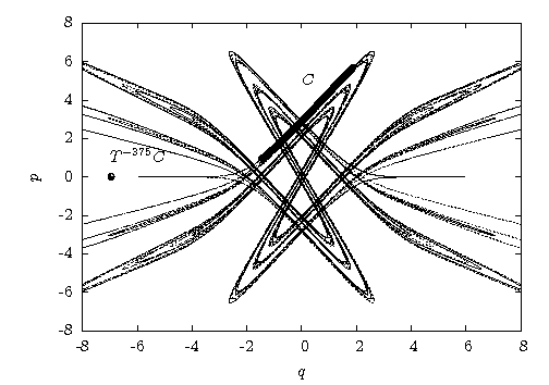
(a) $L=0.00$

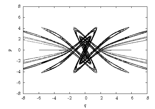
(b) $L=2.60$

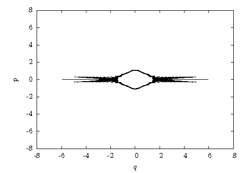
(c) $L=5.71$

Figure 1: The Poincaré Maps for the discrete dynamical system in the axial symmetric case ($A=0$). The $L$ parameter regulates the degree of development of the horseshoe. Notice also reduction of the phase space occupied by the horseshoe as $L$ increases. The line $C$ on 1(a) it’s choosen so that it’s preimage is an adecuate domain for scattering functions.

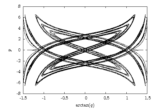
(a) $L=0.00$

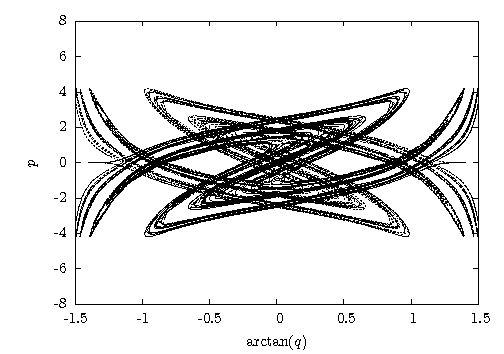
(b) $L=2.60$

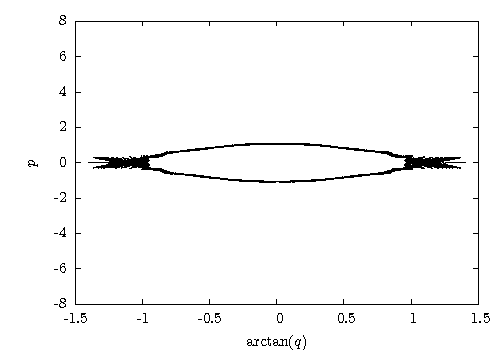
(c) $L=5.71$

Figure 2: Same as fig. 1, but after compactifying the $q$ axis using the function $\arctan(q)$.

To construct the horseshoe we plot the stable manifold and the unstable manifold of both the fixed point at $+\infty$ and of the one at $-\infty$. To plot the whole interval $q\in[-\infty,+\infty]$ on a finite range we use the horizontal coordinate $z=\tanh(q)$ which is convenient to get informative plots (figure 2). The intersection points between a stable and an unstable manifold are trajectories which converge forward in time and also backward in time to a fixed point of the map. An intersection between the manifolds of the same fixed point is called homoclinic point, and an intersection between the manifolds of different fixed points is called heteroclinic point. The whole structure of the manifolds is called homoclinic/heteroclinic tangle, many times only the expression homoclinic tangle or simply tangle is used for short even when it also contains heteroclinic points. The existence of a homoclinic tangle is the topological criterion for chaos in the system. It implies the existence of an uncountable set of unstable trajectories. For more details on the role of homoclinic tangles and the importance for scattering and transport problems see the book by Wiggins [23].

Because of symmetry in our example the manifolds of point $-\infty$ are obtained from the ones of the point at $+\infty$ by inversion about the origin. The time reversal symmetry in the maps permits also to obtain the stable manifolds from the unstable ones by the reflection $p\rightarrow-p$. From those symmetry properties also follows the existence of a trajectory oscillating transverse to the channel at $q=0$. It leads to a fixed point of the map at $q=0$, $p=0$. We call this fixed point the inner fixed point. In total the map has three fixed points where the outer two are symmetry related and therefore we call the resulting homoclinic structure a ternary symmetric horseshoe.

When changing $L$ we have the usual development scenario starting from a complete horseshoe for $L=0$ up to a parabolic line when $L$ reaches its maximal limiting value $L_{max}$ allowed by total energy. In our particular example we have

$$L_{max}=6.23$$ (36)

Next we define the fundamental area $R$ for the horseshoe. Let us start with the local branches of the manifolds of the two outer fixed points and let them grow longer continuously in a completely symmetric pattern. Then at some length we obtain the first intersection points, for symmetry reasons they are located at $q=0$. At this moment let us stop the process of growth. The result is a curvilinear quadrilateral which we call the fundamental rectangle $R$.

The intersection pattern between some local segment of an unstable manifold (e.g. the piece between an outer fixed point and the next corner of $R$) with the whole fractal bundle of stable manifolds already contains the complete information of the whole tangle formed by the manifolds of the outer fixed points, and the knowledge of such local intersection patterns is sufficient. We will make use of this idea for the reconstruction of important properties of the tangle from scattering data. The use of these for determining the development of the horseshoe is profusely explained in [13].

In figure1 a) we included an additional thick line labelled $C$ which runs parallel to one of the local segments of unstable manifolds but just outside of $R$. Note that the intersection pattern between $C$ and the bundle of segments of the stable manifolds coincides exactly with the intersection pattern between the local segment of the unstable manifold and the bundle of segments of stable manifolds. Accordingly also the intersection pattern along line $C$ contains all important information about the whole tangle. The iterated preimages of the line $C$ play an important role in the following as asymptotic initial conditions for scattering trajectories.

Now we will discuss the chaotic structure of the three degrees of freedom system. We begin with $A=0$. Then the surfaces of the various values of $L$ are dynamically independent and we get a fractal structure in the full dimensional domain of the map with its coordinates $q$, $p$, $L$ and $\theta$ in a two step process. First we pile up the tangles for the various values of $L$ obtaining a fractal tangle in a three dimensional embedding space and second we form the Cartesian product of this object with a circle representing the fourth coordinate $\theta$.

For the general three degrees of freedom case we need an argument of robustness of this structure under moderate deformations and moderate breaking of the rotational symmetry. This argument follows from generic transversality properties.

In a system of the form described by the equations 1 and 2, or in the map we obtain a family of horseshoes as depicted in figure 1 in the symmetric case. The development of the horseshoe is indicated by a parameter $\gamma$ which measures the degree to which the horseshoe is developed. $\gamma=0$ is the parabolic line and $\gamma=1$ is the complete ternary symmetric horseshoe, for more explanations and schematic pictures see [13]. In our present case $\gamma$ is a monotonic function of $L$. Accordingly also the value of $L$ orders the pile of two dimensional horseshoes naturally from the complete case, with $L$ near zero, to the integrable system, with $L$ near $L_{max}$. When we view this family of systems as just one geometrical object then the family of invariant manifolds form smooth two dimensional surfaces in the three dimensional embedding space with coordinates $q$, $p$ and $L$. For short we call this structure the three dimensional tangle. Now let us restrict our attention to intersections between the unstable and stable manifolds. The basic pattern is a transverse intersection between two two dimensional surfaces in a three dimensional embedding space as shown schematically in figure 3. A point of interest is that the tangential intersections of the lower dimensional horseshoe become extremal points in $L$ direction of the intersection curve shown in figure 3. The whole curve belongs to the “hyperbolic component” of the invariant set.

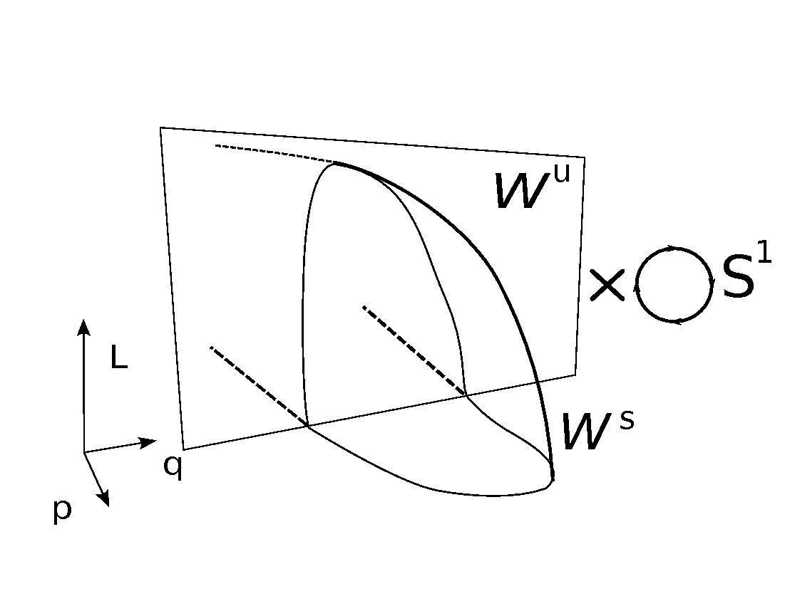
Figure 3: A plot of the intersection of stable and unstable manifolds in the $(p,q,L)$ space when $A=0$. The $L$ value gives the degree of development of the horseshoe for every $(q,p)$ plane. After stacking these in order, we obtain two intersecting two dimensional manifolds. In the end we consider a direct product with a circle for the $\theta$ coordinate.

So far we have ignored the $\theta$ coordinate. To include it for the symmetric case of $A=0$ we simply form the Cartesian product of the structures described above with a circle representing this cyclic coordinate. Thereby the manifolds become three dimensional surfaces in the four dimensional embedding space. The elementary transverse intersection structures between the surfaces $W^{u}$ and $W^{s}$ are smooth two dimensional surfaces. Each one of their points has one dimensional unstable and stable directions and two neutral directions. Because the manifolds themselves are folded to fractal structures we obtain a fractal repetition of the elementary intersection structures which we call the tangle in the four dimensional domain of the Poincaré map. The dimension of this tangle can be anything between two and four depending on how exactly the manifolds turn and fold. For an argument we present later, remember that this dimension is larger than two.

Finally we consider the changes implied by a moderate breaking of the rotational symmetry. To understand this let us return to figure 3 and imagine its product with a circle. Then we see the transverse intersection of two three dimensional surfaces in a four dimensional embedding space. Because the intersection is transverse it is structurally stable. This means, under small deformation the intersection pattern remains qualitatively the same. This argument applies to all the transverse homoclinic intersections appearing in the development scenario of the horseshoe. However, it does not apply to the non hyperbolic structures near the surface of KAM islands.

So, when the parameter $A$ is slightly different from zero, we can understand that relevant qualitative properties of this structure remain unchanged. The structure of the whole four dimensional tangle is therefore robust. This stability, together with the transversality of the intersection, is inherited from the leaves of the symmetric system in a way which is only possible for systems which can be connected continuously to the symmetric systems and which are not far from the symmetric case. This may appear restrictive at first, but even so we can cover a broad range of physically relevant problems.

4 Scattering functions

Scattering functions are interesting objects in their own right and we need them as auxiliary concepts to explain and motivate the ideas on the singularities in the cross sections, which are more accessible to experiments.

A scattering function gives one of the outgoing asymptotic labels, or several of them, as function of initial asymptotic conditions. It is advantageous to study outgoing action like variables as function of initial angular variables, this is exactly the version of the scattering functions we need to understand the properties of the cross sections. As explained before, every asymptotic trajectory in the Poincaré map can be labelled by $p$, $L$, $\psi$ and $\chi$. It is always understood that the total energy $E$ is kept fixed at one particular value.

The scattering function which we will now describe in detail gives the outgoing momentum $p_{out}$ and the angular momentum transfer $\Delta L=L_{out}-L_{in}$ as function of $\chi_{in}$ and $\psi_{in}$ for fixed values of $p_{in}$, $L_{in}$ and $E$. The domain of this function is the 2 dimensional torus with coordinates $\chi_{in}$ and $\psi_{in}$. Periodicity of the function follows thereby.

First let us study the symmetric case $A=0$ and show some numerical examples for the model map. In this case the angle $\psi$ is irrelevant and because of angular momentum conservation the function $\Delta L$ is identically zero. Then the domain of the scattering function is an interval of length $2\pi$ in the angle $\chi_{in}$ and this interval is represented by the line $C$ in figure 1(a). Remember that $C$ is the iterated image of an asymptotic line of fixed $p$ where $q$ changes over an interval of length $p$ which corresponds to an interval of $\chi_{in}$ of length $2\pi$.

As a consequence the scattering function has singularities on a fractal set and intervals of continuity in between. The singularities correspond the intersection of the line of initial conditions with stable manifolds. Since preimages of intersections with invariant manifolds are again intersections with the same manifolds, the intersection pattern of this line of initial conditions coincides with the fractal pattern of intersections of line $C$ with the stable manifolds of the horseshoe. If the asymptotic part of the trajectory starts on a stable manifold of the horseshoe and the actual scattering trajectory converges to a periodic orbit and does not come out of the interaction region with a longitudinal kinetic energy larger than zero, then the outgoing asymptotic conditions are ill defined, and therefore the scattering function has a singularity. The pattern of singularities is the pattern of intersections of the line $C$ with stable manifolds and is a smooth image of the fractal pattern in the tangle. In this way asymptotically obtained scattering functions carry the information on the topological structure of the tangle sitting in the interaction region [13].

We have to ensure that the line of initial conditions maps to a line equivalent to line $C$ in the horseshoe plots and not to a line intersecting the outer tendril further out, where it does not scan the whole structure. As we move line $C$ further away from $R$ we loose more and more intersection points in the line, until it is so far out that it does no longer intersect the bundle of stable manifolds at all. Here it is essential to use a value of $p_{in}$ sufficiently small. The actual line used for the numerical examples of the scattering functions and cross section data will be the 312th preimage of the line $C$ shown in the figure, which is sufficiently far out to be considered asymptotic. This line is given by

$$T^{-312}C=\{(q,p)\|q\in[-6.962,-6.912],p_{in}=0.05\},$$ (37)

where $T$ is the Poincaré Map. If the line of initial conditions intersects the fractal structure only partially, then it still would contain the complete information because of the self-similarity of the fractal structure. However, then the reconstruction would pose some additional technical problems which we want to avoid. Typical structures for the scattering functions on a one dimensional domain are presented in figures 4 and 5.

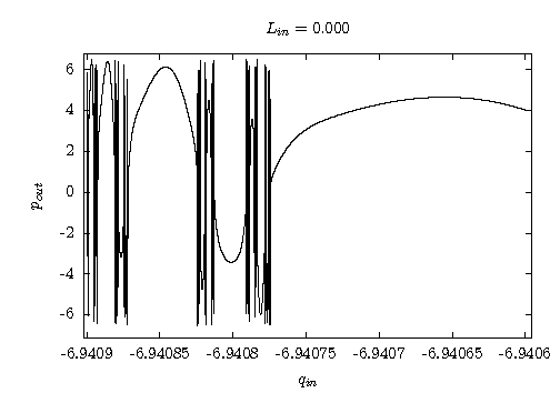
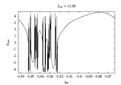
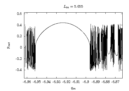
Figure 4: The $p_{out}$ Scattering function for $A=0$ (axial symmetric case). The independent variable is $q_{in}$, the entrance phase.

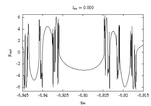
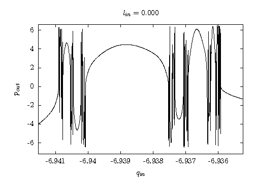
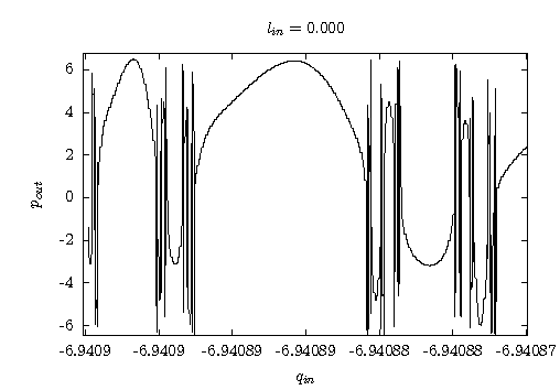
Figure 5: An illustration of the self similarity of the scattering function $p_{out}$ with parameter $L_{in}=0.00$. This case has a complete horseshoe, so the function reveals the structure of a Cantor Set in the singular values.

In a given plot of a scattering function we recognise intersections with the stable manifolds as initial conditions which lead to $p_{out}=0$. They represent boundaries between transmission ($p_{out}>0$) and reflection ($p_{out}<0$).

In preparation for the asymmetric case we have to include the role of the coordinate $\psi$. For $A=0$ the fractal of singularities in the two dimensional domain of the scattering function is the Cartesian product of a one dimensional fractal along the $\chi$ direction described above with a circle in $\psi$ direction. The intervals of continuity have the structure of strips which run in the $\psi$ direction around the domain. The natural domain of the higher dimensional scattering functions is the product of the preimage of the line $C$ described above with the circle of $\psi$ values. It is a two dimensional torus if we recall that the initial and final point of the line $C$ should be identified.

Let us break the rotational symmetry and remember the robustness mentioned at the end of the previous section. For $A$ small the important intervals of continuity have still the same qualitative structure, they are only deformed continuously. Only the non hyperbolic dust around KAM islands is changed immediately for $A\neq 0$. In this sense the qualitative structure of the fractal of singularities is still close to a product of a one dimensional fractal with a circle.

With increasing value of $A$ intervals of increasing size and lower level in the fractal hierarchy are changed qualitatively in so far as they are disrupted into fragments which no longer have the structure of stripes winding around the domain in $\psi$ direction. Only for $A\approx 0.5$ the last large intervals of continuity are destroyed. Thereby the last remnants of the product structure of the fractal are lost and it is transformed into a truly higher dimensional fractal. In the present paper we shall not investigate this new structure, but restrict our consideration to smaller values of $A$.

So far we have seen that all topological information on the chaotic tangle is contained in asymptotic scattering data, and that a measurement of scattering functions and their analysis is one way for the asymptotic observer to obtain this information. The scattering functions present a kind of shadow image of the chaotic invariant set cast into the outgoing asymptotic region. However the measurement of scattering functions is difficult or impossible in many real scattering experiments and therefore we now have to go one step further to cross sections which are the quantity measured in most of the traditional scattering experiments.

5 The cross section

The measurement of scattering functions needs the control over the canonically conjugate variables $p$, $L$ and $\chi$, $\psi$. In classical mechanics this could be done in principle. However, it is not done in the usual scattering experiment. More important, in quantum mechanics this preparation is forbidden even in principle, and if we want to develop concepts and ideas which have some chance to be transferred to quantum dynamics, we can not use quantities needing the simultaneous preparation of canonically conjugate variables. What is done in most scattering experiment is the following: One half of the phase space variables (normally the actions) is prepared as sharp as possible and the other conjugate half (the conjugate angles) is completely unspecified. In our case this means: For fixed total energy $E$ we prepare $p_{in}$ and $L_{in}$ to specific values and do not have any control over the reduced angles $\chi_{in}$ and $\psi_{in}$. Their values have a distribution with constant density over the whole domain, $\mathbb{T}^{2}$. The detector measures the final values $p_{out}$ and $L_{out}$ for each outgoing particle and we monitor the relative probability $\sigma(p_{out},\Delta L)$ to find a given combination of values of $p_{out}$ and $\Delta L$, normalised by the incoming flux. This relative probability is called the doubly differential cross section. For more general information on cross sections see some text book on scattering theory as e.g. [32] or [33], for an application consult [12].

In the previous section we have seen that the scattering function with values $p_{out}(\chi_{in},\psi_{in})$, $\Delta L(\chi_{in},\psi_{in})$ contains the fractal structure of the horseshoe. If we can measure this function directly then we have the necessary data to reconstruct the pattern of the horseshoe and our version of the inverse problem is solved [13]. If we can only measure cross sections we must find out how the fractal pattern of the scattering function is transferred to some recognisable pattern in the cross section.

In the beam of incoming projectiles the weight on the $\chi_{in},\psi_{in}$ torus is constant and the scattering function maps this initial weight on some interval in the range of this function having the coordinates $p_{out}$ and $\Delta L$ and the image weight is exactly the cross section $\sigma(p_{out},\Delta L)$. Therefore to get the value of $\sigma$ for a particular combination of values of $p_{out}$ and $\Delta L$ we first search for all preimages $\chi_{k},\psi_{k}$ of the image point. Each preimage gives the contribution

$$g_{k}(p_{out},\Delta L)=1/|Det\partial(p,\Delta L)/\partial(\chi,\psi)|.$$ (38)

Then the value of the cross section is just the sum of these weights over all the contributing preimage points, i.e:

$$\sigma(p_{out},\Delta L)=\sum_{k}g_{k}(p_{out},\Delta L)$$ (39)

From equation 38 we see that the cross section has singularities at image points where the Jacobian of this map is zero, i.e. points which are locally not invertible. They are caustics of the projection of the graph of the function into the image space. The corresponding singularities in the cross section are called rainbow singularities, for their effect on light scattering off water drops. Now we shall focus on these singularities. Each interval of continuity of the scattering functions leads to one copy of a typical rainbow singularity in the cross section. This gives a possibility to see the fractal structure of the chaotic invariant set in the cross section. For systems with two degrees of freedom this idea has been worked out in detail in [11, 12] and in this section we explain the higher dimensional generalisation.

The determinant of the derivatives of the scattering function is zero exactly for such values of $p_{out}$ and $\Delta L$ for which two trajectories fall together and disappear. Accordingly these singularities are the lines across which the number of contributing trajectories, i.e. the number of preimages changes by 2. Now we will construct a simple analytical normal form for these singularity lines and compare it with numerical results for the three model systems presented in section 2.

First we need an analytical model for the scattering function in one interval of continuity which is as simple as possible but still produces the generic form of singularity in the cross section. As explained in section 4, the domain of the scattering function is the 2 dimensional torus with coordinates $\chi_{in}$ and $\psi_{in}$. For small deviation from symmetry a typical interval of continuity is a strip running around the torus in $\psi$ direction. In $\chi$ direction the strips run in the symmetric case over a limited range only, let us say from $\chi_{0}-\delta$ up to $\chi_{0}+\delta$, where $\chi_{0}$ is the position of the middle of the strip. The value of $p_{out}$ is maximal in the middle of the interval, let us say it has the value $p_{0}$ in the middle, and it goes to zero on the boundaries of the interval of continuity. Accordingly the simplest model function for $p_{out}$ in the symmetric case is

$$p_{out}=p_{0}-(\chi_{0}-\chi_{in})^{2}$$ (40)

where the variables are scaled such that $\delta^{2}=p_{0}$. For the asymmetric case we add a $\psi$ dependent term. This term must be $2\pi$ periodic and for simplicity we take the lowest Fourier contribution only, resulting in

$$p_{out}=p_{0}-(\chi_{0}-\chi_{in})^{2}+b\cos(\psi_{in})$$ (41)

for the general case with broken symmetry. Here for each given value of $\psi$ the variable $\chi$ is restricted to such values which result in a positive value for $p_{out}$. This restriction defines the deformed interval of continuity for the case of broken symmetry.

The function $\Delta L$ is identical zero in the symmetric case. For the case of broken symmetry we will consider first the very simple model function

$$\Delta L=a\sin(\psi_{in})$$ (42)

without $\chi$ dependence and the version with $\chi$ dependence

$$\Delta L=a\sin(\psi_{in})/(1-c(\chi_{in}-\chi_{0}))$$ (43)

The small perturbative parameters $b$ and $c$ will be considered as of the same order.

Now we consider the preimages of these scattering model functions. First, as simplest possibility combine Eqs. 40 and 42. In equation 40 we find 2 possible real preimage values of $\chi$ as long as $p_{out}<p_{0}$ and 0 real preimage values if $p_{out}>p_{0}$. Exactly at $p_{out}=p_{0}$ two preimages collide and turn from real to imaginary, as physical solutions they disappear. Accordingly the line $p_{out}=p_{0}$ is a caustic line in this case. In equation 42 we find 2 real values of $\psi$ for $|\Delta L|<a$ and zero preimages for $|\Delta L|>a$. Along the lines $\Delta L=a$ and $\Delta L=-a$ the two solutions collide and turn from real to imaginary. Therefore also these two lines are caustic lines for this simple case. In total we find 4 preimages inside of the rectangle delimited by the lines $p_{out}=0$, $p_{out}=p_{0}$, $\Delta L=a$ and $\Delta L=-a$ and zero preimages outside of this rectangle (see figure 6). Of course, the caustic structure of this very simple case is not structurally stable, it changes qualitatively under small deformations of the scattering functions. Along generic caustic lines the number of solutions changes by 2 and not by 4. Therefore we need to add the appropriate perturbations to the scattering functions to turn the caustic structure into a structurally stable one. We have to see next that the transitions from equation 40 to equation 41 and from equation 42 to equation 43 are the appropriate perturbations to turn the caustic lines into generic and structurally stable ones.

Next, let us combine Eqs.41 and 42. In this case the function for $\Delta L$ still produces the degenerate caustic lines $\Delta L=a$ and $\Delta L=-a$. If we invert equation 41 and we eliminate the $\psi$ dependence by inserting from equation 42 then we obtain for $\chi$ the equation

$$\chi_{in}=\chi_{0}\pm\sqrt{p_{0}-p_{out}\pm b\sqrt{1-\Delta L^{2}/a^{2}}}$$ (44)

First we see the caustic lines $\Delta L=a$ and $\Delta L=-a$ which are already known from the inversion of equation 42. In addition we also see that solutions collide and turn from real to complex along the ellipse given by the equation

$$a^{2}(p_{0}-p_{out})^{2}+b^{2}\Delta L^{2}=a^{2}b^{2}$$ (45)

In total for the combination of equations 41 and 42 the behaviour of the preimages is the following: Outside of the strip delimited by the lines $\Delta L=a$ and $\Delta L=-a$ the number of real preimages is zero. Let us now look at the interior of this strip. For values of $p_{out}$ outside the ellipse and at the side of larger values we find zero real preimages in $\chi$, inside the ellipse we find 2 preimages and for values of $p_{out}$ between zero and the ellipse we find 4 preimages. The result is: The perturbation introduced in equation 41 is able to modify the degenerate caustic line $p_{out}=p_{0}$ into a structurally stable curve. However, the two caustic curves $\Delta L=a$ and $\Delta L=-a$ stay in their structurally unstable form.

Next let us combine Eqs.40 and 43. The equation40 has the caustic line $p_{out}=p_{0}$ as before. Inserting equation40 into equation43 leads to the following equation for $\psi$

$$\sin(\psi_{in})=\Delta L(1\pm c\sqrt{p_{0}-p_{out}})/a,$$ (46)

which in turn leads to the caustic curves

$$\Delta L=\pm a(1\pm c\sqrt{p_{0}-p_{out}})^{-1}$$ (47)

In the relevant region of $p$ values the curves given by this equation come close to parabolas centred at $\pm a$. Now the preimage structure is the following. We find zero real preimages for $p_{out}>p_{0}$. Therefore let us concentrate on the strip of $p_{out}$ values between zero and the line $p_{out}=p_{0}$. In the region of small values of $\Delta L$ between the two approximate parabolas we find 4 real preimages, inside of the two approximate parabolas we find 2 real preimages and in the rest of the strip zero real preimages. The perturbation introduced in equation43 is able to turn the degenerate caustic lines $\Delta L=a$ and $\Delta L=-a$ into structurally stable curves.

Last, let us check that the combination of Eqs.41, 43 produces structurally stable caustic curves only. Eliminating the variable $\psi_{in}$ and making the substitution $x=\chi_{0}-\chi_{in}$ we get the following polynomial in $x$

$$P(x)=x^{4}+Ax^{2}+Bx+C$$ (48)

where

$$A=2(p_{out}-p_{0})+b^{2}\Delta L^{2}c^{2}/a^{2}$$ (49)

$$B=-2b^{2}\Delta L^{2}c/a^{2}$$ (50)

$$C=(p_{out}-p_{0})^{2}+b^{2}(\Delta L^{2}/a^{2}-1)$$ (51)

In the following we use the abbreviation $D=\Delta L^{2}/a^{2}-1$. A polynomial has colliding solutions whenever its discriminant is zero, see e.g. section II.4 and in particular lemma 4.7 in [34]. In the case of the polynomial of 48 the discriminant is given by

$$\operatorname{Dis}=-27B^{4}-4A^{3}B^{2}+16A^{4}C+144AB^{2}C-128A^{2}C^{2}+256C^{3}$$ (52)

We will evaluate the resulting complicated expression in $p$ and $x$ perturbatively in the small quantities $b$ and $c$. The lowest order contributions come in order 4 and are

$$\operatorname{Dis}_{4}=256b^{4}(p_{out}-p_{0})^{2}D^{2}$$ (53)

This discriminant is zero along the lines $p_{out}=p_{0}$, $\Delta L=a$ and $\Delta L=-a$. All these 3 lines come with multiplicity 2. It is the same caustic structure as we obtained with the combination of the Eqs.40 and 42.

Next we keep all contributions up to order 6 combined in $b$ and $c$ and leave out the irrelevant constant factor $256b^{4}$. The result is

$$\operatorname{Dis}_{6}=b^{2}D^{3}+(p_{out}-p_{0})^{2}D^{2}+2(p_{out}-p_{0})^{3}(\Delta L^{2}/a^{2}+1)\Delta L^{2}c^{2}/a^{2}$$ (54)

The real zeroes of these last expressions in the $(p_{out},\Delta L)$ plane are sketched in figure 6. We have also produced a theoretical plot for the curve of the zeros of the expression 54 with the parameter $a$ set on the value 1 whereas the small parameters $b$ and $c$ take the value 0.1, see the figure 8(d). In these plots the various regions of the plane are marked by the number of real preimages of the original equations 41 and 43. Here all structural instabilities of the caustic curves are removed. Note that this figure coincides with the projection singularities of the ring shaped mountain shown in figure 7. The projection is highlighted on the left side. The parts a, b, c of figure 8 show for comparison the rainbow structure in the cross section coming from a single interval of continuity of the scattering function for the 3 examples introduced in section 2. Part a belongs to the channel with obstacle, part b to the map model and part c to the bottle billiard.

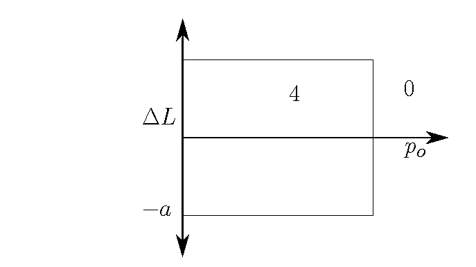
(a) $b=0,c=0$

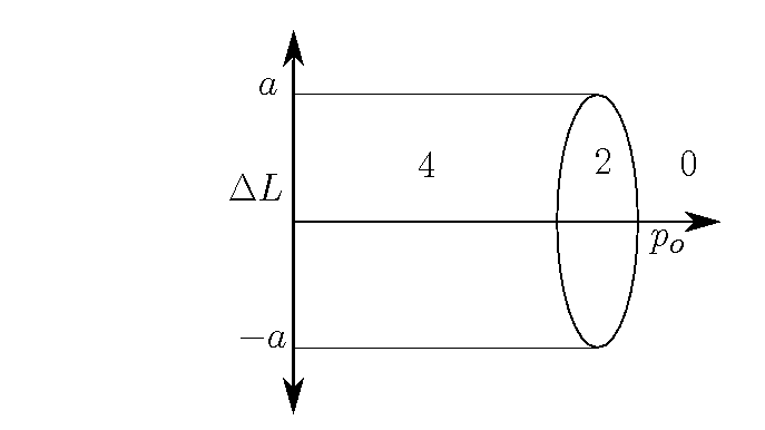
(b) $b\neq 0,c=0$

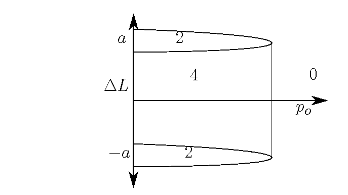
(c) $b=0,c\neq 0$

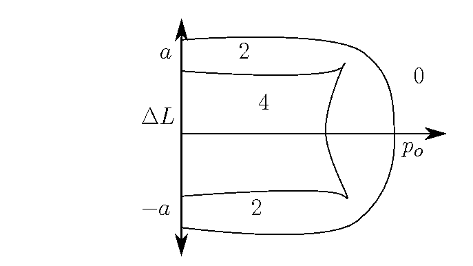
(d) $b\neq 0,c\neq 0$

Figure 6: The diagrams of the regions divided by a rainbow singularity. The numbers indicate the quantity of preimages of the region for each point.

We see: For all the 3 examples the rainbow singularity in the cross section has the same qualitative structure as the curves described by 54. This motivates us to propose 54 as normal form of the rainbow singularity in the double differential cross section for the class of scattering systems considered in this article.

The shape of the normal form induces a ring shaped mountain. Since a ring shaped mountain can be considered half a torus, our projection is half of the well known projection singularity pattern of the torus, see fig. 6.13 of [35].

For moderate breaking of the symmetry each interval of continuity, which is still some strip running around the torus in $\psi$ direction, produces in the cross section one copy of the typical rainbow singularity. Of course, for each individual interval it takes different values of the parameters. The total set of singularities seen in the cross section coming from all intervals is expected to consist of a superposition of a fractal of shifted and continuously deformed copies of the normal form. In principle there should be an infinity of them. Practically we can resolve a finite number up to some finite level of hierarchy of the underlying fractal. Let us turn next to some numerical examples for the cross section.

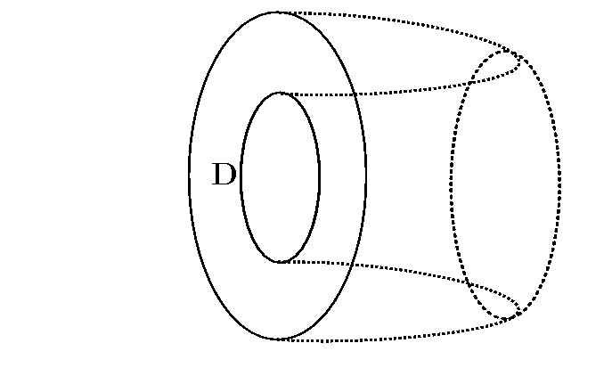
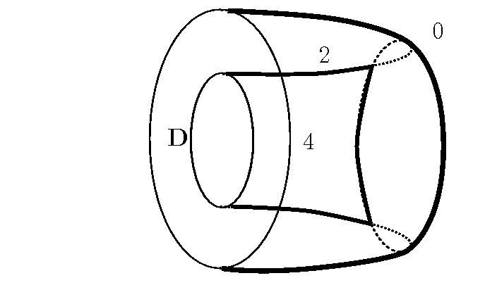
Figure 7: On the left side, labelled 7, we represent an annular region which spans a quadratic maximum. On the right side, 7, we emphasise the singular set of the projection into a two dimensional manifold. The domain of the Scattering function is labelled $D$. The numbers represent the number of inverse preimages for the projection. Compare with figures 6 and 8(d).

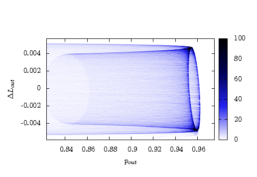
(a) Rainbow Singularity for the channel system.

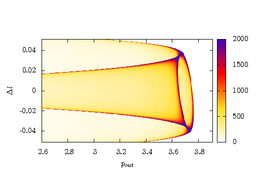
(b) Rainbow Singularity for the map.

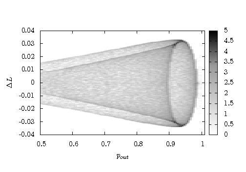
(c) Rainbow Singularity for the billiard.

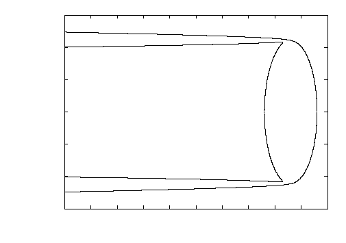
(d) As a comparison, the zeros of the polynomial $Dis_{6}$, equation 54. The parameters are $a=1,b=c=0.1$

Figure 8: Different isolated rainbow singularities corresponding in each case to a single domain of continuity of the scattering functions, for the different systems presented and the solution for the zeros of the $Dis_{6}$ polynomial.

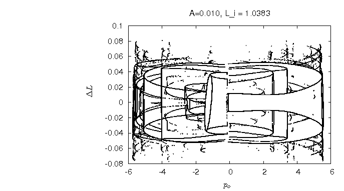
Figure 9: The rainbow singularities for the map system generated by equation 16. The parameters are $A=0.010,L_{in}=1.0383$. We show the structure of the projection of the half torus repeated as far as resolution goes.

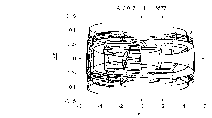
Figure 10: The rainbow singularities for the system generated by the function $G(q,\theta,\tilde{p},\tilde{L})$, (equation 16). The parameters are $A=0.015,L_{in}=1.5575$.

To obtain the figures 8, 9 and 10 we have done a coarse graining of the domain of the cross section which is similar to what any real detector in an experiment does. The domain is divided into many small rectangles and the counts in any one of these rectangles are registered. Each rectangle can be considered one detector channel. High count rates are indicated in the figure by a darker colour. Note that there are high count rates also in some detector channels which do not contain contributions from the true singularity itself, in particular the detector channels near the cusp of the inner singularity line show this behaviour. They are the ones roughly connecting the inner cusp with the outer singularity line and marked by broken lines in figure 7. The high count rates lie along curves which come close to one ellipse and two parabolas, compare with figure 7.

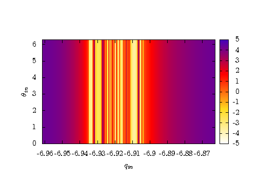
Figure 11: The scattering function for the map generated by the function in expression 16 with $A=0.000$ and $l_{in}=1.0383$ on the torus of initial conditions. As $L$ is conserved, we only show the $p_{out}$ component.

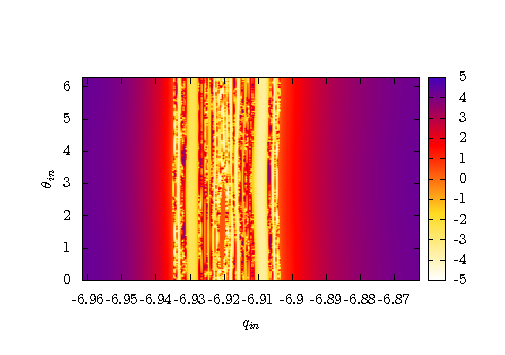
(a) The $p_{out}$ component.

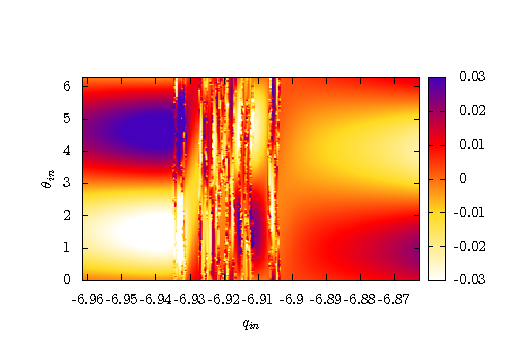
(b) The $\Delta L$ component.

Figure 12: The scattering function for the map generated by the function in expression 16 with $A=0.010$ and $L_{in}=1.0383$ on the torus of initial conditions. This gives the rainbow singularities depicted on figure 9.

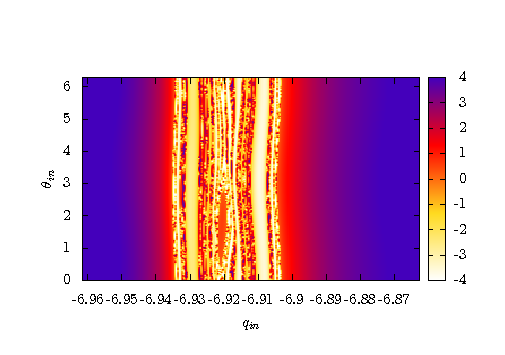
(a) The $p_{out}$ component.

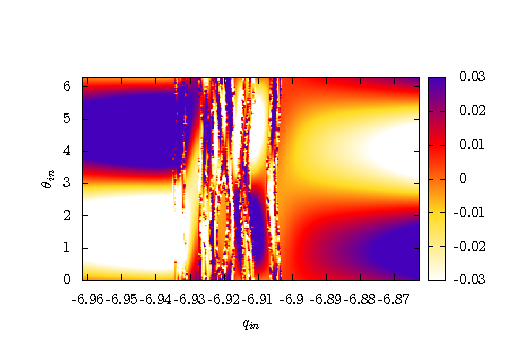
(b) The $\Delta L$ component.

Figure 13: The scattering function for the map generated by the function in expression 16 with $A=0.020$ and $L_{in}=1.0383$ on the torus of initial conditions.

After studying the projections of these points we recognise the shape of the half toroidal mountains, see figures 9, 10. These figures have been obtained by simulating a great quantity of trajectories with initial conditions uniformly distributed on the torus. Then we have selected points on the histogram of final conditions which show a much higher count than their neighbours, as seen on the figures 9 and 10. If we compare them with the black outline on the figure 7, we can see the projection of the same basic repeated over. For a symmetric case we can see the domains of continuity in smoothly changing colours in the figure 11, which partitions the torus into a fractal family of stripes. Each has typically an extremal set of measure zero and shows up as a rainbow singularity in the cross section. As the symmetry gets broken, the embedding remains stable, although the discontinuities bend and may form rings (see figs. 11 and 12), or even multiply punctured domains. Then we observe distinct shapes besides the circular rings which should also represent a complete partition of the domain. It should be noted that the smoother parts of the function have still a ring shaped domain of continuity, and that they are the main contributors to the cross section. Therefore, the experimentally detectable signature of the partitions of the domain is still a family of ring shaped sets.

6 Final remarks

By asymptotic measurements we observe which rainbow contributions are present or absent and can conclude which corresponding intervals of continuity in the scattering function contribute and finally draw conclusions about the structure of the chaotic invariant set in the Poincaré map of the system. In particular we can change a parameter of the system, for example the symmetry breaking parameter A, and follow important changes of the chaotic set, at least in the lower levels of the hierarchy of the fractal structure. For further analysis of the resulting data two promising possibilities exist.

First, we can try to construct a symbolic dynamics for the system. For systems with two degrees of freedom a description of the development scenario of the chaotic set in terms of a development parameter related to an approximate symbolic dynamics has been presented for binary and for ternary symmetric horseshoes in [13] and [36] respectively. This description was based on a rather simple approximation for the symbolic dynamics. In the meantime for chaotic sets of two dimensional maps, more sophisticated approximations for the symbolic dynamics have been developed [37, 38]. It would be worth to generalise all these developments for the four dimensional maps encountered in the present article.

Second, we can measure the weight of the contributions to the structures in cross sections and scattering functions coming from the various levels of hierarchy of the underlying fractal. Thereby we extract scaling factors of this fractal. The distribution of these scaling factors can be analysed by thermodynamical methods to extract the statistical measures of the chaos of the systems. For the thermodynamical methods see [39, 40]. For the application of these methods to chaotic scattering with two degrees of freedom and its cross section see [41].

By knowing which rainbow singularities are present and which ones are missing compared to the complete case and by knowing the scaling factors between contributions from the various levels of the hierarchy we have knowledge about the topology of the horseshoe and about the measures of chaos in two dimensional cases.

All our considerations have been restricted so far to the case where only one degree of freedom is open and all other degrees of freedom are closed. This situation implies the following property of the system: For any value of the total energy the closed degrees of freedom can swallow all energy such that for the open degree of freedom only energy zero remains. Therefore for any positive value of the total energy the motion of the open degree of freedom can come to a stop at infinity ( when the potential is attractive without outer barrier ) or at the outermost potential barrier ( in cases where it exists, where the potential is repulsive for large distances ). In this sense the existence of at least one closed degree of freedom implies that for any positive value of the total energy the system sits exactly on a channel threshold. As a consequence we have the dividing surfaces of dimension 3 ( in the domain of the Poincaré map ) formed by such trajectories and the intersection of the stable and unstable dividing surfaces forms the chaotic set described before. The elementary intersection set between two hyper-surfaces of codimension 1 is a set of codimension 2. If the dividing surfaces form fractal folds, then we have a fractal collection of elementary intersection patterns and the complete intersection set has a codimension less than 2. In our particular case this property guarantees that the chaotic invariant set in the Poincaré map has a dimension larger than 2.

The situation is different if no closed degree of freedom exists. Imagine a system with only open degrees of freedom and an attractive potential. Then for positive values of the total energy it is impossible to have trajectories which go out arbitrarily far and where at the same time the velocity goes to zero. However, such trajectories are exactly the ones which form the homoclinic tangle in the case investigated in the present paper and cause the fractal structure in the scattering functions and in the cross section. This consideration shows that the structures described in this article will not necessarily exist in systems without closed degrees of freedom.

Of course, topological chaos can exist in systems with only open degrees of freedom. One system of this type with 3 degrees of freedom, investigated in the past [25, 42], is scattering of a point particle off four hard spheres situated at the four corners of a tetrahedron. When the radius of the spheres is small compared to their distance then all periodic orbits are completely unstable and we have hyperbolicity. In the 4 dimensional Poincaré map this implies the existence of hyperbolic periodic points but excludes the existence of NHIMs. The invariant manifolds of the hyperbolic points are 2 dimensional, their elementary intersection structures are points. Even when the manifolds are folded to form some fractal structure, the complete intersection structure between stable and unstable manifolds is a fractal built up of points. Then in general the dimension of this intersection structure is small and does not cause much observable structure in scattering functions. According to [25] the intersection structure in the 4 dimensional domain of the Poincaré map should have at least dimension 2 in order to cause easily observable effects in generic scattering functions.

The choice of our class of systems has also favourable consequences for the cross sections. Naturally we look at the doubly differential inelastic cross section as function of two action type variables. In section 5 we studied the cross section as function of angular momentum transfer and of outgoing momentum of the open degree of freedom. Because of conservation of total energy and because of the monotonous dependence of the energy of the oscillating degree of freedom on its action we could equally well express the same cross section as function of angular momentum transfer and the final action of the oscillating degree of freedom. The use of the outgoing momentum has the advantage that its sign indicates immediately whether a particular trajectory describes transmission or reflection. Therefore we stay with the variable $p_{out}$ in the cross section. However, because of the above mentioned considerations we treat $p_{out}$ as if it would be an action variable. Because of energy conservation these two action like variables of the cross section are restricted to a finite interval of possible values. On the boundaries of intervals of continuity of the scattering function $p_{out}$ goes to zero. In the interior of intervals of continuity the scattering function is smooth. Then this function necessarily has generic extrema in the interior and has lines along which the determinant of derivatives is zero. This guarantees the existence of the rainbow structures described above.

Again the situation can be different for scattering systems with open degrees of freedom only. For simplicity think of the scattering of a points particle off a localised potential in a 3 dimensional position space. For the moment consider the rotationally symmetric case where the azimuth angle is irrelevant. Then the possibility exists that in each interval of continuity of the scattering function the deflection angle goes monotonically from minus infinity to plus infinity without any generic extremal points. As has been pointed out in [43] this situation also can happen in cases of chaotic systems. Then the fractal chaotic set in the phase space does not leave fractal traces in the cross section.

What happens for even more degrees of freedom, let say N? We can make some comments for the class of systems where we have one open degree of freedom coupled strongly to one closed degree of freedom and any number of further degrees of freedom which are only coupled weakly to the first two degrees of freedom. Let us assume again that there is a parameter $A$ which gives the strength of this coupling and that we have again a limiting case $A=0$ where these additional degrees of freedom are decoupled from the first two ones and for simplicity also decoupled among themselves and where accordingly the system can be reduced to one with two degrees of freedom. In this case we find a (2N-4) dimensional NHIM in the (2N-2) dimensional domain of the Poincaré map. It is stable in one direction, unstable in one direction and neutrally stable in the remaining (2N-4) directions. The development degree of the horseshoe of the reduced system depends on the amount of energy in the reduced system. Since it depends on the value of the conserved actions of the remaining degrees of freedom we can use one of the remaining neutral directions as development parameter of the horseshoe and in total obtain again a pile of two dimensional horseshoes similar to the 3 dimensional tangle described before for the three degrees of freedom case. In particular we can apply the same arguments of robustness as before. The difference is that now we have to form the Cartesian product of this three dimensional structure with (2N-5) neutral directions, which are partially action directions and partially angle directions. The domain of the scattering function is now a (N-1) dimensional torus of initial relative phase shifts between the N degrees of freedom and its range is a (N-1) dimensional interval of final actions. Take our previous quantities $L$, $\theta$, $\chi$ and $\Delta L$ to be (N-2) component quantities. Under small breaking of the symmetric case $A=0$ the robustness argument indicates again that the coarse structure of the scattering function should be stable, the lower the level of hierarchy in the fractal structure, the more stable the situation should be. The (N-1)-fold differential cross section is the relative probability to obtain some combination of final actions for a constant density of the initial phase shifts. The rainbow singularities are again the projection singularities of the graph of the scattering function under projection on the range. The elementary rainbow structure coming from a single interval of continuity of the scattering function is now a (N-2) dimensional surface in the (N-1) dimensional domain of the cross section. We plan a more detailed discussion of the general case in a future publication.

So far everything has been explained for classical dynamics. Therefore the question remains how our results are reflected in quantum systems, like the ones presented in [44]. We have analysed the cross section as function of the outgoing action for fixed total energy. This was appropriate since classically the actions of the closed degrees of freedom are continuous variables. In this point quantum mechanics is essentially different. In our models asymptotically the open degree of freedom is decoupled from the two closed degrees of freedom, see for example equation 2. Accordingly in the asymptotic region the transverse motion, i.e. the state of the two closed degrees of freedom, must be in one of the discrete quantum states of this bound subsystem. For example in equation 2 the transverse motion is a two dimensional harmonic oscillator with its usual quantization of the action according to $I=(n+1/2)\hbar\omega$. For other particular models of the closed transverse degrees of freedom similar restrictions apply. On the other hand this discreteness of the asymptotic transverse states provide a natural channel decomposition of the S-matrix and the scattering amplitude where we start from a particular asymptotic initial transverse state and study the transitions to the various other energetically allowed final asymptotic transverse states. The open longitudinal degree of freedom does not have similar restrictions, its asymptotic energy can be any positive value. Thus to scan the action of the closed degrees of freedom is impossible in quantum dynamics. The appropriate procedure is to select particular initial and final states of the closed degrees of freedom and to vary the total energy continuously, i.e. study the cross sections for the various channel to channel transitions as function of the total energy. In these quantities we expect to see structures, in particular sequences of scattering resonances, related to the classical chaotic set. So far we did not yet study such implications and they are not the subject of the present publication.

The essential point for the analysis of the quantum mechanical cross section is the wave dynamical analog to classical rainbows. One essential difference between classical dynamics and quantum dynamics is how the contributions from the various initial conditions are summed. In classical dynamics the cross section of equation 39 itself is a sum over the contributing initial conditions. In a semi-classical approximation to quantum dynamics or when using Feynman’s path integral version of the quantum propagator, we first form a scattering amplitude as a sum over contributing trajectories and then form the cross section or scattering probability as absolute square of the amplitude. Therefore the resulting cross section is a double sum over the trajectories and contains first a sum over diagonal terms which has the structure of the classical cross section plus the non diagonal terms which are interferences between the various contributing trajectories. If in a rainbow two trajectories fall together then in a semi classical treatment of the scattering amplitude we have to apply some uniformization which replaces the contribution of the two trajectories by an Airy function. This gives the wave dynamical analog of the classical square root singularity.

Accordingly two things might be done in a wave dynamical treatment. First, the interference pattern in the wave cross section can be analysed. For some attempts in this direction see [41] and [45], where the semi-classical scattering from three soft potential mountains has been used as example of demonstration. Second, a decomposition of the scattering amplitude into Airy type contributions might be tried, in order to recover at least the first few hierarchical levels of the fractal pattern of rainbows. To our knowledge this has not yet been done so far, but might be worth to try.

References

References

- [1] Chaos no. 4. vol. 3, 1993. whole issue.
- [2] C. Jung and S. Pott. Classical cross section for chaotic potential scattering. J. Phys. A, 22:2925, 1989.
- [3] C. Jung and H. J. Scholz. Chaotic scattering off the magnetic dipole. J. Phys. A, 21:2301, 1988.
- [4] B. Eckhardt. Fractal propierties of scattering singularities. Journ. Phys. A, 20:5971, 1987.
- [5] A. Rapoport and V. Rom-Kedar. Chaotic scattering by steep repelling potentials. Phys. Rev. E, 77(016297), 2008.
- [6] K. A. Mitchel and J.B. Delos. The structure of ionizing electron trajectories for hydrogen in parallel fields. Physica D, 229:9, 2007.
- [7] S. Smale. Differentiable dynamical systems. Bul. Am. Math. Soc., 73:747, 1967.
- [8] T. Bütikofer, C. Jung, and T. H. Seligman. Extraction of information about periodic orbits from scattering functions. Phys. Lett. A, 76:265, 2000.
- [9] H. Tapia and C. Jung. Inelastic inverse scattering problem. Phys Lett. A, 198:313, 2003.
- [10] C. Jung, O. Merlo, and T. H. Seligman. Symmetry properties of periodic orbits extracted from scattering data. CHAOS, 14:969, 2005.
- [11] C. Jung, G. Orellana-Rivadeneyra, and G.A. Luna-Acosta. Reconstruction of the chaotic set from classical cross section data. Jour. Phys. A, 38:567, 2004.
- [12] Schelin A.B., de Moura A.P.S, and Grebogi C. Transition to chaotic scattering: Signatures in the differential cross section. Phys. Rev. E., 78:046204, 2008.
- [13] C. Jung, C. Lipp, and T. H. Seligman. The inverse scattering problem for chaotic hamiltonian systems. Annals of Physics, 275:151, 1999.
- [14] A. G. Ramm. Multidimensional Inverse Scattering Problems. Longman Scientific/Wiley, 1992.
- [15] G. M. L. Gladwell. Inverse Problem in Scattering. An Introduction. Kluwer, 1993.
- [16] B. N. Akhariev and A. A. Sucko. Potential and Quantum Scattering. Direct and Inverse Problems. Springer, 1990.
- [17] G. Contopoulos and K. Efstathiou. Escapes and recurrence in a simple hamiltonian system. Cel. Mech. and Dyn. Astron., 88:163, 204.
- [18] H. Waalkens, A. Burbanks, and S. Wiggins. Escape from planetary neighbourhoods. Mon. Not. Roy. Astron. Soc., 361:763, 2005.
- [19] H. Waalkens and S. Wiggins. Geometrical models of the phase space structures governing reaction dynamics. Reg. and Chao. Dyn., 15:1, 2010.
- [20] G. S. Ezra and S. Wiggins. Phase-space geometry and reaction dynamics near index 2 saddles. J. Phys. A, 42(205101), 2009.
- [21] H. Waalkens, R. Schubert, and S. Wiggins. Wigner’s dynamical transition state theory in phase space: classical and quantum. Nonlinearity, 21:R1, 2008.
- [22] T. Uzer, C. Jaffe, J. Palacian, P. Yanguas, and S. Wiggins. The geometry of reactions dynamics. Nonlinearity, 15:957, 2002.
- [23] S. Wiggins. Normally Hyperbolic Invariant Manifolds in Dynamical Systems. Springer Verlag, 1994.
- [24] H . Waalkens, A. Burbanks, and S. Wiggins S. A computational procedure to detect a new type of high-dimensional chaotic saddle and its application to the 3d hill’s problemll. J. Phys A., 37:257, 2004.
- [25] Q. Chen, M. Ding, and E. Ott. Chaotic scattering on several dimensions. Phys. Lett. A, 115:93, 1990.
- [26] L. Benet, J. Broch, O. Merlo, and T. H. Seligman. Symmetry breaking: A heuristic approach to chaotic scattering in many dimensions. Phys. Rev. E, 71:036225, 2005.
- [27] B. Dietz, T. Papenbrock B. Mößner, U. Reif, and A. Richter. Bouncing ball orbits and symmetry breaking effects in a three-dimensional chaotic billiard. Phys. Rev. E, 77:046221, 2008.
- [28] E. A. Jackson. Perspectives of nonlinear dynamics. Cambridge University Press, 1989.
- [29] C. Jung, C. Mejia-Monasterio, O. Merlo, and T. H. Seligman. Self pulsing effect in chaotic scattering. New J. Phys., 6:48, 2004.
- [30] Paul Hansen, Kevin A. Mitchell, and John B. Delos. Escape of trajectories from a vase-shaped cavity. Phys. Rev. E, 73(6):066226, 2006.
- [31] N. Chernov and R. Markarian. Chaotic Billiards, volume 127. Mathematical Surveys and Monographs, 2006.
- [32] J. R. Taylor. Scattering Theory. Wiley, 1972.
- [33] R. G. Newton. Scattering Theory of Waves and Particles. Springer, 1982.
- [34] K. Kendig. Elementary Algebraic Geometry. Springer, 1977.
- [35] A. M. Ozorio de Almeida. Hamiltonian Systems: Chaos und Quantization. Cambridge Univeristy Press, 1988.
- [36] B. Rückerl and C. Jung. Scaling propierties of a scattering system with an incomplete horseshoe. J. Phys. A, 27:55, 1994.
- [37] K. A. Mitchell and J. B. Delos. A new topological technique for characterizing homoclinic tangles. Physica D, 221:170, 2006.
- [38] K. A. Mitchell. The topology of nested homoclinic and heteroclinic tangles. Physica D, 238:737, 2009.
- [39] T. Tel. Directions in Chaos, chapter 3. World Scientific, 1990.
- [40] C. Beck and F. Schlögel. Thermodynamics of Chaotic Systems. Cambridge University Press, 1993.
- [41] C. Jung and T. Tel. Dimension and escape rate of chaotic scattering from classical and semiclassical cross section data. J. Phys. A, 24:2793, 1991.
- [42] H. J. Korsch and A. Wagner. Fractal mirror images and chaotic scattering. Comp. in Phys., 5:497, 1991.
- [43] A. P. de Moura and C. Grebogi. Rainbow transition in chaotic scattering. Phys. Rev. E, 65:035206, 2002.
- [44] K. A. Mitchell and B Ilan. Nonlinear enhancement of the fractal structure in the escape dynamics of bose-einstein condensates. Phys. Rev. A, 80(043406), 2009.
- [45] C. Jung. Fractal properties in the semiclassical scattering cross section of a classically chaotic system. J. Phys A., 23:1217, 1990.