Accelerating a FFT-based solver for numerical homogenization of periodic media by conjugate gradients

Abstract

In this short note, we present a new technique to accelerate the convergence of a FFT-based solver for numerical homogenization of complex periodic media proposed by Moulinec and Suquet [1]. The approach proceeds from discretization of the governing integral equation by the trigonometric collocation method due to Vainikko [2], to give a linear system which can be efficiently solved by conjugate gradient methods. Computational experiments confirm robustness of the algorithm with respect to its internal parameters and demonstrate significant increase of the convergence rate for problems with high-contrast coefficients at a low overhead per iteration.

url]http://mech.fsv.cvut.cz/~zemanj

1 Introduction

A majority of computational homogenization algorithms rely on the solution of the unit cell problem, which concerns the determination of local fields in a representative sample of a heterogeneous material under periodic boundary conditions. Currently, the most efficient numerical solvers of this problem are based on discretization of integral equations. In the case of particulate composites with smooth bounded inclusions embedded in a matrix phase, the problem can be reduced to internal interfaces and solved with remarkable accuracy and efficiency by the fast multipole method, see [3, and references therein]. An alternative method has been proposed by Suquet and Moulinec [1] to treat problems with general microstructures supplied in the form of digital images. The algorithm is based on the Neumann series expansion of the inverse to an operator arising in the associated Lippmann-Schwinger equation and exploits the Fast Fourier Transform (FFT) to evaluate the action of the operator efficiently.

The major disadvantage of the FFT-based method consists in its poor convergence for composites exhibiting large jumps in material coefficients. To overcome this difficulty, Eyre and Milton proposed in [4] an accelerated scheme derived from a modified integral equation treated by means of the series expansion approach. In addition, Michel et al. [5] introduced an equivalent saddle-point formulation solved by the Augmented Lagrangian method. As clearly demonstrated in a numerical study by Moulinec and Suquet [6], both methods converge considerably faster than the original variant; the number of iterations is proportional to the square root of the phase contrast instead of the linear increase for the basic scheme. However, this comes at the expense of increased computational cost per iteration and the sensitivity of the Augmented Lagrangian algorithm to the setting of its internal parameters.

In this short note, we introduce yet another approach to improve the convergence of the original FFT-based scheme [1] based on the trigonometric collocation method [7] and its application to the Helmholtz equation as introduced by Vainikko [2]. We observe that the discretization results in a system of linear equations with a structured dense matrix, for which a matrix-vector product can be computed efficiently using FFT, cf. Section 2. It is then natural to treat the resulting system by standard iterative solvers, such as the Krylov subspace methods, instead of the series expansion technique. In Section 3, the potential of such approach is demonstrated by means of a numerical study comparing the performance of the original scheme and the conjugate- and biconjugate-gradient methods for two-dimensional scalar electrostatics.

2 Methodology

In this section, we briefly summarize the essential steps of the trigonometric collocation-based solution to the unit cell problem by adapting the original exposition by Vainikko [2] to the setting of electrical conduction in periodic composites. In what follows, $a$, ${\boldsymbol{a}}$ and ${\boldsymbol{A}}$ denote scalar, vector and second-order tensor quantities with Greek subscripts used when referring to the corresponding components, e.g. $A_{\alpha\beta}$. Matrices are denoted by a serif font (e.g. $\mathsf{A}$) and a multi-index notation is employed, in which $\mathbb{R}^{\mathbb{{\boldsymbol{N}}}}$ with ${\boldsymbol{N}}=(N_{1},\ldots,N_{d})$ represents $\mathbb{R}^{N_{1}\times\cdots\times N_{d}}$ and $\mathsf{A}^{\boldsymbol{k}}$ stands for the $(k_{1},\ldots,k_{d})$-th element of the matrix $\mathsf{A}\in\mathbb{R}^{\boldsymbol{N}}$.

2.1 Problem setting

We consider a composite material represented by a periodic unit cell $\mathcal{Y}=\prod_{\alpha=1}^{d}(-Y_{\alpha},Y_{\alpha})\subset\mathbb{R}^{d}$. In the context of linear electrostatics, the associated unit cell problem reads as

$${\boldsymbol{\nabla}}\times{\boldsymbol{e}}({\boldsymbol{x}})={\boldsymbol{0}}, {\boldsymbol{\nabla}}\cdot{\boldsymbol{j}}({\boldsymbol{x}})={\boldsymbol{0}}, {\boldsymbol{j}}({\boldsymbol{x}})={\boldsymbol{L}}({\boldsymbol{x}})\cdot{\boldsymbol{e}}({\boldsymbol{x}}),\;{\boldsymbol{x}}\in\mathcal{Y}$$ (1)

where ${\boldsymbol{e}}$ is a $\mathcal{Y}$-periodic vectorial electric field, ${\boldsymbol{j}}$ denotes the corresponding vector of electric current and ${\boldsymbol{L}}$ is a second-order positive-definite tensor of electric conductivity. In addition, the field ${\boldsymbol{e}}$ is subject to a constraint

$${\boldsymbol{e}}^{0}=\frac{1}{\left|\mathcal{Y}\right|}\int_{\mathcal{Y}}{\boldsymbol{e}}({\boldsymbol{x}})\,{\mathrm{d}}{\boldsymbol{x}},$$ (2)

where ${\boldsymbol{e}}^{0}$ denotes a prescribed macroscopic electric field and $\left|\mathcal{Y}\right|$ represents the $d$-dimensional measure of $\mathcal{Y}$.

Next, we introduce a homogeneous reference medium with constant conductivity ${\boldsymbol{L}}^{0}$, leading to a decomposition of the electric current field in the form

$${\boldsymbol{j}}({\boldsymbol{x}})={\boldsymbol{L}}^{0}\cdot{\boldsymbol{e}}({\boldsymbol{x}})+\delta{\boldsymbol{L}}({\boldsymbol{x}})\cdot{\boldsymbol{e}}({\boldsymbol{x}}), \delta{\boldsymbol{L}}({\boldsymbol{x}})={\boldsymbol{L}}({\boldsymbol{x}})-{\boldsymbol{L}}^{0}.$$ (3)

The original problem (1)–(2) is then equivalent to the periodic Lippmann-Schwinger integral equation, formally written as

$${\boldsymbol{e}}({\boldsymbol{x}})+\int_{\mathcal{Y}}{\boldsymbol{\Gamma}}^{0}({\boldsymbol{x}}-{\boldsymbol{y}})\cdot\Bigl{(}\delta{\boldsymbol{L}}({\boldsymbol{y}})\cdot{\boldsymbol{e}}({\boldsymbol{y}})\Bigr{)}\,{\mathrm{d}}{\boldsymbol{y}}={\boldsymbol{e}}^{0}, {\boldsymbol{x}}\in\mathcal{Y},$$ (4)

where the ${\boldsymbol{\Gamma}}^{0}$ operator is derived from the Green’s function of the problem (1)–(2) with ${\boldsymbol{L}}({\boldsymbol{x}})={\boldsymbol{L}}^{0}$ and ${\boldsymbol{e}}^{0}={\boldsymbol{0}}$. Making use of the convolution theorem, Eq. (4) attains a local form in the Fourier space:

$$\widehat{{\boldsymbol{e}}}({\boldsymbol{k}})=\left\{\begin{array}[]{rl}\left|\mathcal{Y}\right|^{\frac{1}{2}}{\boldsymbol{e}}^{0},&{\boldsymbol{k}}={\boldsymbol{0}},\\ \displaystyle-\widehat{{\boldsymbol{\Gamma}}}^{0}({\boldsymbol{k}})\cdot\widehat{\left(\delta{\boldsymbol{L}}\cdot{\boldsymbol{e}}\right)}({\boldsymbol{k}}),&{\boldsymbol{k}}\in\mathbb{Z}^{d}\backslash\{{\boldsymbol{0}}\},\end{array}\right.$$ (5)

where $\widehat{f}({\boldsymbol{k}})$ denotes the Fourier coefficient of $f({\boldsymbol{x}})$ for the ${\boldsymbol{k}}$-th frequency given by

$$\widehat{f}({\boldsymbol{k}})=\int_{\mathcal{Y}}f({\boldsymbol{x}})\varphi_{-{\boldsymbol{k}}}({\boldsymbol{x}})\,{\mathrm{d}}{\boldsymbol{x}}, \varphi_{{\boldsymbol{k}}}({\boldsymbol{x}})=|\mathcal{Y}|^{-\frac{1}{2}}\exp\left(\mathrm{i}\pi\sum_{\alpha=1}^{d}\frac{x_{\alpha}k_{\alpha}}{Y_{\alpha}}\right),$$ (6)

”$\mathrm{i}$” is the imaginary unit and

$$\widehat{{\boldsymbol{\Gamma}}}^{0}({\boldsymbol{k}})=\left\{\begin{array}[]{rl}{\boldsymbol{0}},&{\boldsymbol{k}}={\boldsymbol{0}},\\ \displaystyle\frac{{\boldsymbol{k}}\otimes{\boldsymbol{k}}}{{\boldsymbol{k}}\cdot{\boldsymbol{L}}^{0}\cdot{\boldsymbol{k}}},&{\boldsymbol{k}}\in\mathbb{Z}^{d}\backslash\{{\boldsymbol{0}}\},\end{array}\right.$$ (7)

Here, we refer to [4, 8] for additional details.

2.2 Discretization via trigonometric collocation

Numerical solution of the Lippmann-Schwinger equation is based on a discretization of a unit cell $\mathcal{Y}$ into a regular periodic grid with $N_{1}\times\cdots\times N_{d}$ nodal points and grid spacings ${\boldsymbol{h}}=(2Y_{1}/N_{1},\ldots,2Y_{d}/N_{d})$. The searched field ${\boldsymbol{e}}$ in (4) is approximated by a trigonometric polynomial ${\boldsymbol{e}}^{\boldsymbol{N}}$ in the form (cf. [2])

$${\boldsymbol{e}}({\boldsymbol{x}})\approx{\boldsymbol{e}}^{\boldsymbol{N}}({\boldsymbol{x}})=\sum_{{\boldsymbol{{\boldsymbol{k}}}}\in\mathbb{Z}^{{\boldsymbol{N}}}}\widehat{{\boldsymbol{e}}}({\boldsymbol{k}})\varphi_{{\boldsymbol{k}}}({\boldsymbol{x}}), {\boldsymbol{x}}\in\mathcal{Y},$$ (8)

where ${\boldsymbol{N}}=(N_{1},\ldots,N_{d})$, $\widehat{{\boldsymbol{e}}}$ designates the Fourier coefficients defined in (6) and

$$\mathbb{Z}^{{\boldsymbol{N}}}=\left\{{\boldsymbol{k}}\in\mathbb{Z}^{d}:-\frac{N_{\alpha}}{2}<k_{\alpha}\leq\frac{N_{\alpha}}{2},\alpha=1,\ldots,d\right\}.$$ (9)

We recall, e.g. from [2], that the $\alpha$-th component of the trigonometric polynomial expansion $e_{\alpha}^{\boldsymbol{N}}$ admits two equivalent finite-dimensional representations. The first one is based on a matrix $\widehat{\mathsf{e}}_{\alpha}\in\mathbb{C}^{{\boldsymbol{N}}}$ of the Fourier coefficients of the $\alpha$-th component and equation (8) with $\widehat{e}_{\alpha}({\boldsymbol{k}})=\widehat{\mathsf{e}}_{\alpha}^{\boldsymbol{k}}$. Second, the data can be entirely determined by interpolation of nodal values

$$e^{\boldsymbol{N}}_{\alpha}({\boldsymbol{x}})=\sum_{{\boldsymbol{k}}\in\mathbb{Z}^{{\boldsymbol{N}}}}\mathsf{e}_{\alpha}^{{\boldsymbol{k}}}\varphi^{\boldsymbol{N}}_{{\boldsymbol{k}}}({\boldsymbol{x}}), \alpha=1,\ldots,d$$ (10)

where $\mathsf{e}_{\alpha}\in\mathbb{R}^{\boldsymbol{N}}$ is a matrix storing electric field values at grid points, $\mathsf{e}_{\alpha}^{{\boldsymbol{k}}}=e^{\boldsymbol{N}}_{\alpha}({\boldsymbol{x}}^{\boldsymbol{k}})$ is the corresponding value at the ${\boldsymbol{k}}$-th node with coordinates ${\boldsymbol{x}}^{\boldsymbol{k}}=(k_{1}h_{1},\ldots,k_{d}h_{d})$ and basis functions

$$\varphi^{\boldsymbol{N}}_{{\boldsymbol{k}}}({\boldsymbol{x}})=|{\boldsymbol{N}}|^{-1}\sum_{{\boldsymbol{m}}\in\mathbb{Z}^{{\boldsymbol{N}}}}\exp\left\{\mathrm{i}\pi\sum_{\alpha=1}^{d}m_{\alpha}\left(\frac{x_{\alpha}}{Y_{\alpha}}-\frac{2k_{\alpha}}{N_{\alpha}}\right)\right\}$$ (11)

satisfy the Dirac delta property $\varphi^{\boldsymbol{N}}_{{\boldsymbol{k}}}({\boldsymbol{x}}^{\boldsymbol{m}})=\delta_{{\boldsymbol{m}}{\boldsymbol{k}}}$ with $\left|{\boldsymbol{N}}\right|=\prod_{\alpha=1}^{d}N_{\alpha}$. Both representations can be directly related to each other by

$$\widehat{\mathsf{e}}_{\alpha}=\mathsf{F}\mathsf{e}_{\alpha}, \mathsf{e}_{\alpha}=\mathsf{F}^{-1}\widehat{\mathsf{e}}_{\alpha},$$ (12)

where the Vandermonde matrices $\mathsf{F}\in\mathbb{C}^{{\boldsymbol{N}}\times{\boldsymbol{N}}}$ and $\mathsf{F}^{-1}\in\mathbb{C}^{{\boldsymbol{N}}\times{\boldsymbol{N}}}$

$$\mathsf{F}^{{\boldsymbol{k}}{\boldsymbol{m}}} = |\mathcal{Y}|^{-\frac{1}{2}}\exp\left(-\sum_{\alpha=1}^{d}2\pi\mathrm{i}\frac{k_{\alpha}m_{\alpha}}{N_{\alpha}}\right),$$ (13)

$$\left(\mathsf{F}^{-1}\right)^{{\boldsymbol{k}}{\boldsymbol{m}}} = |\mathcal{Y}|^{\frac{1}{2}}|{\boldsymbol{N}}|^{-1}\exp\left(\sum_{\alpha=1}^{d}2\pi\mathrm{i}\frac{k_{\alpha}m_{\alpha}}{N_{\alpha}}\right),$$ (14)

implement the forward and inverse Fourier transform, respectively, e.g. [9, Section 4.6].

The trigonometric collocation method is based on the projection of the Lippmann-Schwinger equation (4) to the space of the trigonometric polynomials of the form $\left\{\sum_{{\boldsymbol{k}}\in\mathbb{Z}^{{\boldsymbol{N}}}}c_{\boldsymbol{k}}\varphi_{\boldsymbol{k}},c_{\boldsymbol{k}}\in\mathbb{C}\right\}$, cf. [7, 2]. In view of Eq. (10), this is equivalent to the collocation at grid points, with the action of ${\boldsymbol{\Gamma}}^{0}$ operator evaluated from the Fourier space expression (5) converted to the nodal representation by (12)₂. The resulting system of collocation equations reads

$$\left(\mathsf{I}+\mathsf{B}\right)\mathsf{e}=\mathsf{e}^{0},$$ (15)

where $\mathsf{e}\in\mathbb{R}^{d\times{\boldsymbol{N}}}$ and $\mathsf{e}^{0}\in\mathbb{R}^{d\times{\boldsymbol{N}}}$ store the corresponding solution and of the macroscopic field, respectively. Furthermore, $\mathsf{I}$ is the $d\times d\times{\boldsymbol{N}}\times{\boldsymbol{N}}$ unit matrix and the non-symmetric matrix $\mathsf{B}$ can be expressed, for the two-dimensional setting, in the partitioned format as

$$\mathsf{B}=\left[\begin{array}[]{cc}\mathsf{F}^{-1}&\mathsf{0}\\ \mathsf{0}&\mathsf{F}^{-1}\end{array}\right]\left[\begin{array}[]{cc}\widehat{\mathsf{\Gamma}}^{0}_{11}&\widehat{\mathsf{\Gamma}}^{0}_{12}\\ \widehat{\mathsf{\Gamma}}^{0}_{21}&\widehat{\mathsf{\Gamma}}^{0}_{22}\end{array}\right]\left[\begin{array}[]{cc}\mathsf{F}&\mathsf{0}\\ \mathsf{0}&\mathsf{F}\end{array}\right]\left[\begin{array}[]{cc}\mathsf{\delta\mathsf{L}}_{11}&\mathsf{\delta\mathsf{L}}_{12}\\ \mathsf{\delta\mathsf{L}}_{21}&\mathsf{\delta\mathsf{L}}_{22}\end{array}\right],$$ (16)

with an obvious generalization to an arbitrary dimension. Here, $\widehat{\mathsf{\Gamma}}^{0}_{\alpha\beta}\in\mathbb{R}^{{\boldsymbol{N}}\times{\boldsymbol{N}}}$ and $\mathsf{\delta\mathsf{L}}_{\alpha\beta}\in\mathbb{R}^{{\boldsymbol{N}}\times{\boldsymbol{N}}}$ are diagonal matrices storing the corresponding grid values, for which it holds

$$\left(\widehat{\mathsf{\Gamma}}^{0}_{\alpha\beta}\right)^{{\boldsymbol{k}}{\boldsymbol{k}}}=\widehat{\Gamma}^{0}_{\alpha\beta}({\boldsymbol{k}}), \displaystyle\mathsf{\delta\mathsf{L}}^{{\boldsymbol{k}}{\boldsymbol{k}}}_{\alpha\beta}=\delta L_{\alpha\beta}({\boldsymbol{x}}^{\boldsymbol{k}}), \alpha,\beta=1,\ldots,d\mbox{ and }{\boldsymbol{k}}\in\mathbb{Z}^{{\boldsymbol{N}}}.$$ (17)

2.3 Iterative solution of collocation equations

It follows from Eq. (16) that the cost of the multiplication by $\mathsf{B}$ or by $\mathsf{B}^{\mathsf{T}}$ is driven by the forward and inverse Fourier transforms, which can be performed in $O(\left|{\boldsymbol{N}}\right|\log\left|{\boldsymbol{N}}\right|)$ operations by FFT techniques. This makes the resulting system (15) ideally suited for iterative solvers.

In particular, the original Fast Fourier Transform-based Homogenization (FFTH) scheme formulated by Moulinec and Suquet in [1] is based on the Neumann expansion of the matrix inverse $(\mathsf{I}+\mathsf{B})^{-1}$, so as to yield the $m$-th iterate in the form

$$\mathsf{e}^{(m)}=\sum_{j=0}^{m}\left(-\mathsf{B}\right)^{j}\mathsf{e}^{0}.$$ (18)

Convergence of the series (18) was comprehensively studied in [4, 8], where it was shown that the optimal rate of convergence is achieved for

$${\boldsymbol{L}}^{0}=\frac{\lambda_{\min}+\lambda_{\max}}{2}{\boldsymbol{I}},$$ (19)

with $\lambda_{\min}$ and $\lambda_{\max}$ denoting the minimum and maximum eigenvalues of ${\boldsymbol{L}}({\boldsymbol{x}})$ on $\mathcal{Y}$ and ${\boldsymbol{I}}$ being the identity tensor.

Here, we propose to solve the non-symmetric system (15) by well-established Krylov subspace methods, in particular, exploiting the classical Conjugate Gradient ($\mathrm{CG}$) method [10] and the biconjugate gradient ($\mathrm{BiCG}$) algorithm [11]. Even though that $\mathrm{CG}$ algorithm is generally applicable to symmetric and positive-definite systems only, its convergence in the one-dimensional setting has been proven by Vondřejc [12, Section 6.2]. A successful application of $\mathrm{CG}$ method to a generalized Eshelby inhomogeneity problem has also been recently reported by Novák [13] and Kanaun [14].

3 Results

To assess the performance of the conjugate gradient algorithms, we consider a model problem of the transverse electric conduction in a square array of identical circular particles with $50\%$ volume fraction. A uniform macroscopic field ${\boldsymbol{e}}^{0}=(1,0)$ is imposed on the corresponding single-particle unit cell, discretized by ${\boldsymbol{N}}=(255,255)$ nodes and the phases are considered to be isotropic with the conductivities set to ${\boldsymbol{L}}={\boldsymbol{I}}$ for the matrix phase and to ${\boldsymbol{L}}=\varrho{\boldsymbol{I}}$ for the particle.

The conductivity of the homogeneous reference medium is parameterized as

$${\boldsymbol{L}}^{0}(\omega)=\left(1-\omega+\varrho\omega\right){\boldsymbol{I}},$$ (20)

where $\omega=0.5$ corresponds to the optimal convergence of $\mathrm{FFTH}$ algorithm (19). All conjugate gradient-related results have been obtained using the implementations according to [16] and referred to as Algorithm 6.18 ($\mathrm{CG}$ method) and Algorithm 7.3 ($\mathrm{BiCG}$ scheme). Two termination criteria are considered. The first one is defined for the $m$-th iteration as [15]

$$\left(\eta_{\rm e}^{(m)}\right)^{2}=\frac{\sum_{{\boldsymbol{k}}\in\mathbb{Z}^{{\boldsymbol{N}}}}\left({\boldsymbol{k}}\cdot\widehat{\mathsf{j}}^{{\boldsymbol{k}}(m)}\right)^{2}}{\|\widehat{\mathsf{j}}^{{\boldsymbol{0}}(m)}\|^{2}_{2}}\leq\varepsilon^{2},$$ (21)

and provides the test of the equilibrium condition (1)₂ in the Fourier space. An alternative expression, related to the standard residual norm for iterative solvers, has been proposed by Vinogradov and Milton in [8] and admits the form

$$\eta_{\rm r}^{(m)}=\frac{\|\mathsf{L}^{0}\left(\mathsf{e}^{(m+1)}-\mathsf{e}^{(m)}\right)\|_{2}}{\|\mathsf{e}^{0}\|_{2}}\leq\varepsilon,$$ (22)

with the additional $\mathsf{L}^{0}$ term ensuring the proportionality to (21) at convergence. From the numerical point of view, the latter criterion is more efficient than the equilibrium variant, which requires additional operations per iteration. From the theoretical point of view, its usage is justified only when supported by a convergence result for the iterative algorithm. In the opposite case, the equilibrium norm appears to be more appropriate, in order to avoid spurious non-physical solutions.

3.1 Choice of reference medium and norm

Since no results for the optimal choice of the reference medium are known for $\mathrm{(Bi)CG}$-based solvers, we first estimate their sensitivity to this aspect numerically. The results appear in Fig. 1, plotting the relative number of iterations for $\mathrm{CG}$ and $\mathrm{BiCG}$ solvers against the conductivity of the reference medium parameterized by $\omega$, recall Eq. (20).

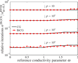
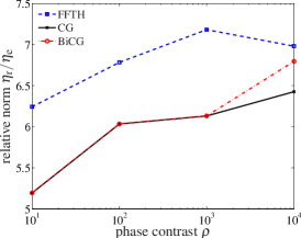
Figure 1: (a) Relative number of iterations as a function of the reference medium parameter $\omega$ and (b) ratio between residual- and equilibrium-based norms at convergence for $\eta_{\rm r}$ termination condition with tolerance $\varepsilon=10^{-4}$.

As expected, both $\mathrm{CG}$ and $\mathrm{BiCG}$ solvers achieve a significant improvement over $\mathrm{FFTH}$ method in terms of the number of iterations, ranging from $50\%$ for a mildly-contrasted composite down to $2\%$ for $\varrho=10^{4}$. Moreover, contrary to all other available methods, the number of iterations is almost independent of the choice of the reference medium. We also observe, in agreement with results by [12, Section 6.2] for the one-dimensional setting, that $\mathrm{CG}$ and $\mathrm{BiCG}$ algorithms generate identical sequences of iterates; the minor differences visible for $\omega>1$ or $\varrho=10^{4}$ can be therefore attributed to accumulation of round-off errors. These conclusions hold for both equilibrium- and residual-based norms, which appear to be roughly proportional for the considered range of the phase contrasts, cf. Fig. 1. Therefore, the residual criterion (22) will mostly be used in what follows.

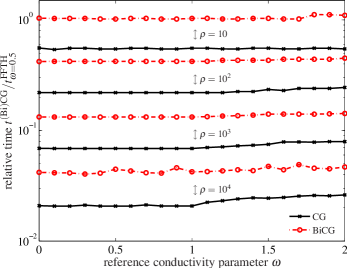
Figure 2: Relative CPU time $t$ of $\mathrm{CG}$ and $\mathrm{BiCG}$ solvers plotted against the conductivity parameter $\omega$ for $\eta_{\rm r}$-based termination condition with tolerance $\varepsilon=10^{-4}$.

In Fig. 2, we supplement the comparison by considering the total CPU time required to achieve a convergence. The data indicate that the cost of one iteration is governed by the matrix-vector multiplication, recall Eq. (16): the overhead of $\mathrm{CG}$ scheme is about $10\%$ with respect to $\mathrm{FFTH}$ method, while the application of $\mathrm{BiCG}$ algorithm, which involves $\mathsf{B}$ and $\mathsf{B}^{\mathsf{T}}$ products per iteration [11], is about twice as demanding. As a result, CG algorithm significantly reduces the overall computational time in the whole range of contrasts, whereas a similar effect has been reported for the candidate schemes only for $\varrho\geq 10^{3}$, cf. [6].

3.2 Influence of phase contrast

As confirmed by all previous works, the phase contrast $\varrho$ is the critical parameter influencing the convergence of FFT-based iterative solvers. In Fig. 3, we compare the scaling of the total number of iterations with respect to phase contrast for CG and $\mathrm{FFTH}$ methods, respectively. The results clearly show that the number of iterations grows as $\sqrt{\varrho}$ instead of the linear increase for $\mathrm{FFTH}$ method. This follows from error bounds

$$\eta_{\rm r}^{(m)}\leq\gamma^{m}\eta_{\rm r}^{(0)}, \displaystyle\gamma^{\mathrm{FFTH}}=\frac{\varrho-1}{\varrho+1}, \gamma^{\mathrm{CG}}=\frac{\sqrt{\varrho}-1}{\sqrt{\varrho}+1}.$$ (23)

The first estimate was proven in [4], whereas the second expression is a direct consequence of the condition number of matrix $\mathsf{B}$ being proportional to $\varrho$ and a well-known result for the conjugate gradient method, e.g. [16, Section 6.11.3]. The CG-based method, however, failed to converge for the infinite contrast limit. Such behavior is equivalent to the Eyre-Milton scheme [4]. It is, however, inferior to the Augmented Lagrangian algorithm, for which the convergence rate improves with increasing $\rho$ and the method converges even as $\rho\rightarrow\infty$. Nonetheless, such results are obtained for optimal, but not always straightforward, choice of the parameters [5].

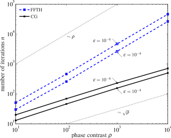
Figure 3: Total number of iterations $n$ plotted against phase contrast $\varrho\,$; the reference medium corresponds to for $\omega=0.5$ and tolerance $\varepsilon$ is related to $\eta_{\rm r}$ norm.

3.3 Convergence progress

The final illustration of the $\mathrm{CG}$-based algorithm is provided by Fig. 4, displaying a detailed convergence behavior for both low- and high-contrast cases. The results in Fig. 4 correspond well with estimates (23) for both residual and equilibrium-based norms. Influence of a higher phase contrast is visible from Fig. 4, plotted in the full logarithmic scale. For $\mathrm{FFTH}$ algorithm, two regimes can be clearly distinguished. In the first few iterations, the residual error rapidly decreases, but the iterates tend to deviate from equilibrium. Then, both residuals are simultaneously reduced. For $\mathrm{CG}$ scheme, the increase of the equilibrium residual appears only in the first iteration and then the method rapidly converges to the correct solution. However, its convergence curve is irregular and the algorithm repeatedly stagnates in two consecutive iterations. Further analysis of this phenomenon remains a subject of future work.

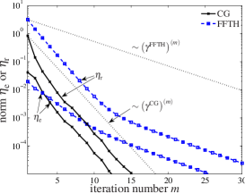
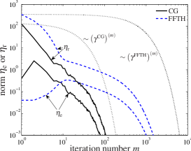
Figure 4: Convergence progress of CG and FFTH methods for (a) $\varrho=10^{1}$ and (b) $\varrho=10^{3}$ as quantified by $\eta_{\rm e}$ and $\eta_{\rm r}$ norms; reference medium corresponds to $\omega=0.5$ and the dot-and-dahsed curves indicate the convergence rates (23).

4 Conclusions

In this short note, we have presented a conjugate gradient-based acceleration of the FFT-based homogenization solver originally proposed by Moulinec and Suquet [1] and illustrated its performance on a problem of electric conduction in a periodic two-phase composite with isotropic phases. On the basis of obtained results, we conjecture that:

• the non-symmetric system of linear equations (15), arising from discretization by the trigonometric collocation method [2], can be solved using the standard conjugate gradient algorithm,

• the convergence rate of the method is proportional to the square root of the phase contrast,

• the methods fails to converge in the infinite contrast limit,

• contrary to available improvements of the original FFT-solver [4, 5], the cost of one iteration remains comparable to the basic scheme and the method is insensitive to the choice of auxiliary reference medium.

The presented computational experiments provide the first step towards further improvements of the method, including a rigorous analysis of its convergence properties, acceleration by multi-grid solvers and preconditioning and the extension to non-linear problems.

Acknowledgements

The authors thank Milan Jirásek (Czech Technical University in Prague) and Christopher Quince (University of Glasgow) for helpful comments on the manuscript. This research was supported by the Czech Science Foundation, through projects No. GAČR 103/09/1748, No. GAČR 103/09/P490 and No. GAČR 201/09/1544, and by the Grant Agency of the Czech Technical University in Prague through project No. SGS OHK1-064/10.

References

- [1] H. Moulinec, P. Suquet, A fast numerical method for computing the linear and nonlinear mechanical properties of composites, Comptes rendus de l’Académie des sciences. Série II, Mécanique, physique, chimie, astronomie 318 (11) (1994) 1417–1423.
- [2] G. Vainikko, Fast solvers of the Lippmann-Schwinger equation, in: R. P. Gilbert, J. Kajiwara, Y. S. Xu (Eds.), Direct and Inverse Problems of Mathematical Physics, Vol. 5 of International Society for Analysis, Applications and Computation, Kluwer Academic Publishers, Dordrecht, The Netherlands, 2000, pp. 423–440.
- [3] L. Greengard, J. Lee, Electrostatics and heat conduction in high contrast composite materials, Journal of Computational Physics 211 (1) (2006) 64–76.
- [4] D. J. Eyre, G. W. Milton, A fast numerical scheme for computing the response of composites using grid refinement, The European Physical Journal Applied Physics 6 (1) (1999) 41–47.
- [5] J. C. Michel, H. Moulinec, P. Suquet, A computational method based on augmented Lagrangians and fast Fourier transforms for composites with high contrast, CMES-Computer Modeling in Engineering & Sciences 1 (2) (2000) 79–88.
- [6] H. Moulinec, P. Suquet, Comparison of FFT-based methods for computing the response of composites with highly contrasted mechanical properties, Physica B: Condensed Matter 338 (1–4) (2003) 58–60.
- [7] J. Saranen, G. Vainikko, Trigonometric collocation methods with product integration for boundary integral equations on closed curves, SIAM Journal on Numerical Analysis 33 (4) (1996) 1577–1596.
- [8] V. Vinogradov, G. W. Milton, An accelerated FFT algorithm for thermoelastic and non-linear composites, International Journal for Numerical Methods in Engineering 76 (11) (2008) 1678–1695.
- [9] G. Golub, C. F. Van Loan, Matrix Computations, The Johns Hopkins University Press, Baltimore and London, 1996.
- [10] M. R. Hestenes, E. Stiefel, Methods of conjugate gradients for solving linear systems, Journal of Research of the National Bureau of Standards 49 (6) (1952) 409–463.
- [11] R. Fletcher, Conjugate gradient methods for indefinite systems, in: G. Watson (Ed.), Numerical Analysis, Proceedings of the Dundee Conference on Numerical Analysis, 1975, Vol. 506 of Lecture Notes in Mathematics, Springer-Verlag, New York, 1976, pp. 73–89.
- [12] J. Vondřejc, Analysis of heterogeneous materials using efficient meshless algorithms: One-dimensional study, Master’s thesis, Czech Technical University in Prague (2009). http://mech.fsv.cvut.cz/~vondrejc/download/ING.pdf
- [13] J. Novák, Calculation of elastic stresses and strains inside a medium with multiple isolated inclusions, in: M. Papadrakakis, B. Topping (Eds.), Proceedings of the Sixth International Conference on Engineering Computational Technology, Stirlingshire, UK, 2008, p. 16 pp, paper 127. doi:10.4203/ccp.89.127
- [14] S. Kanaun, Fast calculation of elastic fields in a homogeneous medium with isolated heterogeneous inclusions, International Journal of Multiscale Computational Engineering 7 (4) (2009) 263–276.
- [15] H. Moulinec, P. Suquet, A numerical method for computing the overall response of nonlinear composites with complex microstructure, Computer Methods in Applied Mechanics and Engineering 157 (1–2) (1998) 69–94.
- [16] Y. Saad, Iterative Methods for Sparse Linear Systems, 2nd Edition, Society for Industrial and Applied Mathematics, Philadelphia, PA, USA, 2003.