From Frictional to Viscous Behavior: Three Dimensional Imaging and Rheology of Gravitational Suspensions

Abstract

We probe the three dimensional flow structure and rheology of gravitational (non-density matched) suspensions for a range of driving rates in a split-bottom geometry. We establish that for sufficiently slow flows, the suspension flows as if it were a dry granular medium, and confirm recent theoretical modelling on the rheology of split-bottom flows. For faster driving, the flow behavior is shown to be consistent with the rheological behavior predicted by the recently developed “inertial number” approaches for suspension flows.

Flows of granular materials submersed in a liquid of unequal density have started to attract considerable attention Coussot et al. (1999); Lemaitre et al. (2009); Cassar et al. (2005); Siavoshi et al. (2006); Pailha and Pouliquen (2009) and are relevant in many practical applications Frey and Church (2009). These materials, which we will refer to as “gravitational” suspensions, clearly differ from density matched suspensions, which have been studied in great detail Jomha et al. (1991); Stickel and Powell (2005); Fall et al. (2009); Einstein (1905). Gravitational suspensions exhibit sedimentation, large packing fractions and jamming of the material, which suggests a description similar to dry granular matter Jaeger et al. (1996); Forterre and Pouliquen (2008).

In the last two decades, various flow regimes have been identified for dry granular matter. Sufficiently slow flows are frictional: the ratio of shear (driving) to normal (confining) stresses becomes independent of flow rate if the material is allowed to dilate Tardos et al. (1998); Forterre and Pouliquen (2008). Faster flows are referred to as inertial: here the effective friction coefficient $\mu$ depends on the so-called ”inertial” number $I$, which is a non-dimensional measure of the local flow rate MiDi (2004); Forterre and Pouliquen (2008); Jop et al. (2006).

For gravitational suspensions, the presence of liquid instead of gas as interstitial medium strongly affects the microscopic picture — how should we think of the flow of such suspensions? Pouliquen and coworkers proposed that the ratio of the strain rate and settling time, $I_{S}$, would play a similar role as the inertial number in dry granular flows Pailha and Pouliquen (2009). They furthermore conjectured a dependence of the effective friction coefficient $\mu$ on $I_{S}$ similar to the dry case, and applied this rheological law to capture the behavior of underwater avalanches Pailha et al. (2008).

Here we test this picture by combining 3D imaging and rheological measurements of the flow of gravitational suspensions in a so-called split-bottom geometry (Fig. 1). This geometry has two main advantages. First, the flow rate, which is the key control parameter in the inertial number framework, can be varied over several orders of magnitude, allowing us to access slow flows as seen in plane shear Siavoshi et al. (2006); Divoux and Géminard (2007), faster flows as seen in gravity driven flows Pailha and Pouliquen (2009); Doppler et al. (2007), and the crossover regime in between - something not achieved in previous studies of gravitational suspensions Siavoshi et al. (2006); Divoux and Géminard (2007); Pailha and Pouliquen (2009); Doppler et al. (2007). Second, extensive experimental and numerical work Fenistein and van Hecke (2003); Fenistein et al. (2004, 2006); Cheng et al. (2006); Depken et al. (2007); Ries et al. (2007) has shown that the split bottom geometry produces highly nontrivial slow dry granular flows. A simple frictional picture is not sufficient to capture these flows Dijksman et al. (2004); Sakaie et al. (2004), so that testing whether these profiles also arise in slowly sheared gravitational suspensions is a stringent test for similarities between slow dry flows and slow gravitational suspension flows.

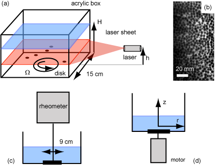
Figure 1: (Color online) (a) The experimental setup used for flow visualization in a ”‘split-bottom”’ geometry. (b) Example image of a single cross section, displaying half the box. (c) Geometry used for rheological measurements.(d) Geometry used for flow visualization.

Setup — The split-bottom geometry is sketched in Fig. 1a, and consists of a square box, 15 cm in width with transparent acrylic walls, at the (rough) bottom of which a (rough) disk of radius $R_{s}=4.5$ cm can be rotated at rate $\Omega$.

We use monodisperse acrylic spheres with a diameter $d$ of 4.6 mm (Engineering Labs); all our results are qualitatively similar for 3.2 mm particles. The particles are suspended in a mixture of some 78% Triton X-100, 13 % water, and 9% ZnCl2 (by weight) Dijksman et al. with a fluorescent dye added (Nile Blue 690). The refractive indices of particles and fluid are approximately 1.49 and match closely — we adapted the recipe from Krishnan et al. (1996). The fluids viscosity $\eta_{f}$ is 0.3 ($\pm 0.05$) Pa s, and the difference in density between the fluid and the particles is about 100 kg/m³.

The particle motion is visualized by illuminating the suspension with a thin ( $<200\mu$m ) laser sheet Siavoshi et al. (2006); Tsai et al. (2003); Slotterback et al. (2008). The laser (Stocker Yale, 635 nm) is aligned parallel to the bottom of the box (Fig. 1a) and mounted on a z-stage which allows the illumination of slices of the suspension at different heights $h$ Slotterback et al. (2008). Image acquisition is done with a triggered 12 bit cooled CCD camera, and contrast is sufficient to image half of the box (Fig. 1b). We use a Particle Image Velocimetry-like (PIV) method to obtain the normalized azimuthal velocity $\omega(r,z)=v_{\theta}/(r\Omega)$ in slices of constant $z$. Combining these slices, we reconstruct the full angular velocity field as function of radius and depth for a range of driving rates. An overview of the imaging technique will be published elsewhere Dijksman et al. .

Rheological experiments were carried out by driving the disk from above with a rheometer (Anton Paar MCR 501) — see Fig. 1c. Velocimetry measurements were done by driving the disk from below with a DC motor — see Fig. 1d. There is always at least half a centimeter of fluid above the suspension to ensure that the surface tension of the fluid will not affect the dilation Tardos et al. (1998) of the packing.

Constitutive equation — We derive the constitutive equation for our suspension in the modified ”inertial number” approach Cassar et al. (2005). The typical rearrangement timescale for the particles in the suspension, given the viscosity and relative density of the particles becomes $d/v_{\inf}=\eta_{f}/P\alpha$, where $v_{\inf}$, $P$ and $\alpha$ are settling velocity, pressure and porosity, so that the ’inertial number’ becomes: $I_{S}=\frac{\dot{\gamma}\eta_{f}}{P\alpha}$  Cassar et al. (2005). The shear stress stress $\tau$ is then written as $\tau=\mu(I)P$, with $\mu(I)$ an empirical friction function. For small $I$, $\mu(I)$ can be expanded: $\mu(I)=\mu_{0}+\mu_{1}I$  Cassar et al. (2005); Koval et al. (2009); Pailha and Pouliquen (2009), with $\mu_{0}$ and $\mu_{1}$ empirical values. Combining this with the expression for $I_{S}$, we arrive at:

$$\tau=\mu_{0}P+\mu_{1}\frac{\eta_{f}\dot{\gamma}}{\alpha}$$ (1)

Thus, to lowest order, the local stress in a gravitational suspension is a linear combination of a frictional stress and a purely viscous stress Pailha and Pouliquen (2009). This is reminiscent of the rheology of a Bingham fluid, in that slow flows are rate independent while faster flows become dominated by simple viscous drag. There is, however, a crucial difference: for slow driving, the shear stresses are predicted to be proportional to the pressure, while only for faster flows, the shear stresses become asymptotically independent of pressure.

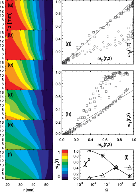
Figure 2: (Color online) Frictional to viscous crossover in flow profiles. (a) The predicted flow field for dry granular flows $\omega_{D}(r,z)$ from Refs. Fenistein and van Hecke (2003); Fenistein et al. (2004, 2006); Cheng et al. (2006); Depken et al. (2007); Ries et al. (2007); Dijksman et al. (2004). (b-e) Measured velocity fields $\omega_{S}(r,z)$ at driving rates $\Omega=8.3\times 10^{-5}$ rps (b), $\Omega=8.3\times 10^{-4}$ rps (c) , $8.3\times 10^{-3}$ rps (d) and $8.3\times 10^{-2}$ rps (e). (f) The Newtonian flow field $\omega_{N}(r,z)$ calculated with the finite element method (see text). Note the similarity of (a) to (b) and (e) to (f). (g) Scatter plot comparison of $\omega_{D}(r,z)$ (a) and $\omega_{S}(r,z)$ for $\Omega=8.3\times 10^{-5}$ rps ($\Box$)(a) and $\Omega=8.3\times 10^{-2}$ rps ($\circ$). (h) Scatter plot comparison of $\omega_{S}(r,z)$ and the flow field of a Newtonian flow $\omega_{N}(r,z)$ for $\Omega=8.3\times 10^{-5}$ rps ($\Box$) and $\Omega=8.3\times 10^{-2}$ rps ($\circ$). (i) $\chi^{2}$ vs $\Omega$ for comparison to granular ($\triangle$) and Newtonian flow ($\star$). The flow characteristics change from granular to Newtonian with increasing shear rate.

Flow profiles — In Fig. 2a-f we compare, for a range of driving rates, the measured flow fields, $\omega_{S}(r,z)$ (panel b-e) with predicted flow fields for dry granular media (panel a) and Newtonian flow (panel f). We fix the particle filling height at 23 mm $(H/R_{S}\approx 0.5)$. Clearly the flow structure progressively changes for faster flow rates, as the defining characteristic of slow flows, the trumpet-like co-rotating inner core, disappears completely. This change is qualitative in nature, with a transition from concave to convex shapes of the iso-velocity lines. In addition we note an increase of slip near the driving disk — while for slow flows, the normalized angular velocity $\omega_{S}$ reaches 1 near the disk, for the fastest flow $\omega_{S}$ has a maximum of 0.7.

The predicted flow field $\omega_{D}(r,z)$ for slow dry flows with $H/R_{s}\approx 0.5$ is shown in Fig. 2a – see equations 1,2,6 and 7 from Ref Dijksman et al. (2004). The similarity to the slowest flow profile, Fig. 2b, $\Omega=8.3\times 10^{-5}$ rps, is striking, and is confirmed in a scatter plot of $\omega_{S}(r,z)$ vs $\omega_{D}(r,z)$, where all data for $\Omega=8.3\times 10^{-5}$ rps (square) collapses on a straight line — see Fig. 2g. We conclude that the flow profiles of slowly sheared gravitational suspension and dry granular media are indistinguishable.

The predicted flow field $\omega_{N}(r,z)$ for Newtonian flows with $H/R_{s}\approx 0.5$ is determined by a finite element software package (COMSOL) to solve the steady state Navier-Stokes equations for an incompressible Newtonian fluid, and is shown in Fig. 2f. The similarity between the measured suspension flows for large $\Omega$ and the Newtonian flow is, again, striking, and is confirmed in a scatter plot of $\omega_{S}(r,z)$ vs $\omega_{N}(r,z)$, where all data for $\Omega=8.3\times 10^{-2}$ rps (circles) tends to a straight line (Fig. 2h).

The crossover from frictional to viscous behavior can be quantified further by calculating as function of $\Omega$ the total mean squared deviation ($\chi^{2}$) obtained from a linear fit of the measured flow profiles $\omega_{S}(r,z)$ to the predicted dry ($\omega_{D}(r,z)$) and viscous ($\omega_{N}(r,z)$) flows, as shown in Fig. 2i. We conclude that the flow profiles of gravitational suspensions show a crossover from frictional, granular behavior to viscous flow upon increasing the driving rate.

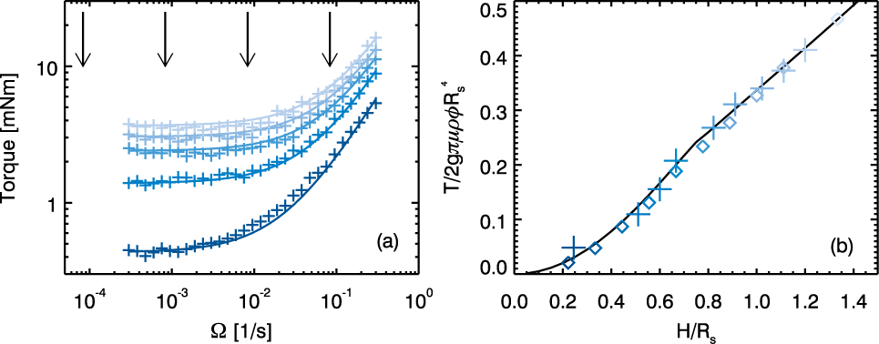
Figure 3: (Color online) (a) Rheology of 4.6 mm acrylic particles in pure Triton X-100. $T(\Omega)$ for a $H/R_{s}=$ 0.24, 0.51, 0.60, 0.67, 0.82, 0.91, 1.0, 1.1, 1.2; color (intensity) indicates $H/R_{s}$. $\Omega=3.0\times 10^{-4}$ to $0.3$. The curve is a fit of the form $T=T_{0}+C\Omega$ (see text). The four arrows indicate the driving rates where flow profiles were measured. (b) $T_{0}(H)$, the plateau values as a function $H$ compared to the prediction from Eq. 2 with $\mu=0.57\pm 0.03$ for the dry ($\diamond$) and $\mu=0.59\pm 0.03$ for the suspension (+) case.

Rheology — Can we find the same crossover between these two regimes in the rheology? We measure the average driving torque as a function of filling height $H$ and driving rate $\Omega$, in order to connect the rheology to the findings for the flow profiles discussed above note_01 . Since index matching is not necessary, we use pure Triton X-100 as interstitial fluid; we use the same particles as before and keep the temperature fixed at 25^∘. In each experiment, $\Omega$ is incremented from low to high values; each data point is obtained by averaging over three or more rotations (transients occur over much smaller strains).

In Fig. 3a we show $T(H,\Omega)$ for several different suspension filling heights. We conclude that the trends in the rheology are similar for all filling heights. First, we observe a rate independent regime at small $\Omega$, which corresponds to the range where we observed flow profiles similar to the dry case. Moreover, the overall stress depends on filling height, which we will show below to be consistent with a pressure dependence. Second, the stresses become rate dependent for $\Omega\sim 0.01$ rps, and for larger rotation rates, the torque increases linearly with $\Omega$; over the whole range of driving rates explored, the rheological data can be well fitted as $T=T_{0}+C\Omega$, consistent with the behavior predicted by Eq. (1) note_01 . We note here that a comparison of the measured torque for pure Triton and for the suspension yields that the effective viscosity of the suspension is only three to five times larger than $\eta_{f}$. This is far below than what would naively be expected from textbook formulae, e.g., Krieger-Dougherty. We have no explanation for this, but note that in the nontrivial split bottom geometry, the suspension packing fraction varies throughout the material Dijksman et al. (2004), which complicates the analysis.

We will now show that the height dependent torque for slow flows, $T_{0}(H)$, is well described by a prediction originally developed for slow dry flows (Fig. 3b). From Eq.1 it follows that the rheology should be determined by the local hydrostatic pressure and an effective friction coefficient $\mu_{0}$. Unger and coworkers Unger et al. (2004) used these ingredients to predict $r(z)$, the center of the shear band of the dry split-bottom flow profiles, but their model also gives a prediction for $T(H)$:

$$T(H)=2g\pi\rho\phi\mu_{0}\int_{0}^{H}(H-z)r^{2}\sqrt{1+(dr/dz)^{2}}dz.$$ (2)

Here $\rho$ is the density of the particles, corrected for buoyancy in case of submersed particles, $\phi$ is the average packing fraction ($\sim 0.59$ Forterre and Pouliquen (2008)) and $\mu_{0}$ is the effective friction coefficient. Minimization of Eq. 2 yields a prediction for $T(H)$ which has not been tested previously.

As shown in Fig. 3b this prediction agrees very well with our measurements. The single fit parameter in the model allows to accurately extract a friction coefficient, which we estimate as $\mu_{0}\sim 0.59\pm 0.03$. We carried out the same measurement of $T(H)$ on dry acrylic particles (Fig. 3b) and obtain a friction coefficient of $\mu_{0}=0.57\pm 0.03$. The two friction coefficients are identical to within the experimental error, a fact also observed in Ref. Divoux and Géminard (2007). This is strong evidence that in the slow driving rate limit the suspension behaves as a dry granular material and that lubrication and other hydrodynamic effects can be ignored. Furthermore, we can conclude that the simple frictional model by Unger correctly captures the overall stresses.

We have also tested the scaling in the viscous regime, by measuring the rheology of glass beads ($\rho$ = 2.5 $\times 10^{3}$ kg/m³) immersed to $H/R_{S}=0.4$ in glycerol for temperatures between 4 and 37 ${}^{\circ}C$. The viscosity of the glycerol mixture varies more than a decade over this temperature range, and hence should change the rotation rate at which the viscous regime sets in. The results are shown in Fig. 4. Eq. (1) requires that the data can be rescaled with the viscosity of the liquid $\eta_{f}$ — this is indeed observed in the inset of Fig. 4. Note that the growth of torque with strain rate over the larger range probed here is somewhat slower than the simple linear prediction note_01 .

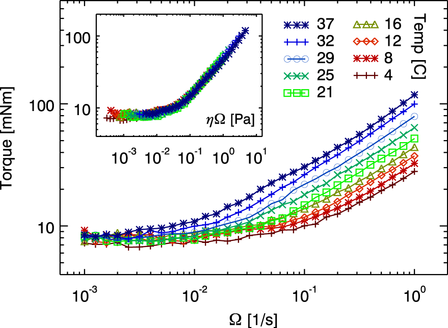
Figure 4: (Color online) The rheology of glass beads in a glycerol mixture at different temperatures. The inset shows the same data, with the abscissa rescaled with the viscosity of the glycerol at the given temperatures.

Conclusions — Our main finding is that with increasing shear rate, a gravitational suspension crosses over from flowing like a dry granular material to flowing like a viscous liquid, consistent with recent modelling of suspensions based on the inertial number approach. We observe this both in the full three dimensional flow profile, which we revealed using an index matched scanning technique, and in rheological measurements. Most of our data can be understood based on simple scaling arguments (to obtain the “transition” shear rate) or elegant minimization principles (to obtain $\mu$ from $T(H)$). Our measurements indicate that the shape and width of the shear band in slow suspensions are the same as for slow dry granular flows. Whatever the physics beyond friction necessary to produce these flow profiles, our data shows that it is equally present in both dry granular and gravitational suspension flows. Still, a simple physical argument for the most prominent feature of split-bottom shear flows — the large width and error function shape of the shear zone Fenistein and van Hecke (2003); Fenistein et al. (2004, 2006); Cheng et al. (2006); Depken et al. (2007) — remains elusive.

Acknowledgement: This work was supported by NSF-CTS0625890 and NSF-DMR0907146. JAD, EW and MvH acknowledge funding from the Dutch physics foundation FOM. We thank Krisztian Ronaszegi for the design and construction of the 3D imaging system of the split-bottom shear cell, and Jeroen Mesman for outstanding technical assistance in the construction of the rheological setup.

References

- Coussot et al. (1999) C. Ancey and P. Coussot, C.R. Acad. Paris 327, 515 (1999).
- Cassar et al. (2005) C. Cassar, M. Nicolas, and O. Pouliquen, Phys. Fluids 17, 103301 (2005).
- Siavoshi et al. (2006) S. Siavoshi, A. V. Orpe, and A. Kudrolli, Phys. Rev. E 73, 010301 (2006).
- Lemaitre et al. (2009) A. Lemaitre, J.-N. Roux, and F. Chevoir, Rheol. Acta 48, 925 (2009).
- Pailha and Pouliquen (2009) M. Pailha and O. Pouliquen, J. Fluid Mech. 633, 115 (2009).
- Frey and Church (2009) P. Frey and M. Church, Science 325, 1509 (2009).
- Jomha et al. (1991) A. Jomha et. al., Powder Techn. 65, 343 (1991).
- Stickel and Powell (2005) J. J. Stickel and R. Powell, Annu. Rev. Fluid Mech. 37, 129 (2005).
- Fall et al. (2009) A. Fall, F. Bertrand, G. Ovarlez, and D. Bonn, Phys. Rev. Lett. 103, 178301 (2009).
- Einstein (1905) A. Einstein, Ann. Physik 19, 289 (1905).
- Jaeger et al. (1996) H. M. Jaeger, S. R. Nagel, and R. P. Behringer, Rev. Mod. Phys. 68, 1259 (1996).
- Forterre and Pouliquen (2008) Y. Forterre and O. Pouliquen, Annu. Rev. Fluid Mech. 40, 1 (2008).
- Tardos et al. (1998) G. I. Tardos, M. I. Khan, and D. G. Schaeffer, Phys. Fluids 10, 335 (1998).
- MiDi (2004) G. MiDi, Eur. Phys. J. E 14, 341 (2004).
- Jop et al. (2006) P. Jop, Y. Forterre, and O. Pouliquen, Nature 441, 727 (2006).
- Pailha et al. (2008) M. Pailha, M. Nicolas, and O. Pouliquen, Phys. Fluids 20, 111701 (2008).
- Divoux and Géminard (2007) T. Divoux and J.-C. Géminard, Phys. Rev. Lett. 99, 258301 (2007).
- Doppler et al. (2007) D. Doppler et. al., J. Fluid Mech. 577, 161 (2007).
- Fenistein and van Hecke (2003) D. Fenistein and M. van Hecke, Nature 425, 256 (2003).
- Fenistein et al. (2004) D. Fenistein, J.-W. van de Meent, and M. van Hecke, Phys. Rev. Lett. 92, 094301 (2004).
- Fenistein et al. (2006) D. Fenistein, J.-W. van de Meent, and M. van Hecke, Phys. Rev. Lett. 96, 118001 (2006).
- Cheng et al. (2006) X. Cheng et. al. Phys. Rev. Lett. 96, 038001 (2006).
- Depken et al. (2007) M. Depken et. al., EPL 78, 58001 (2007).
- Ries et al. (2007) A. Ries, D. E. Wolf, and T. Unger, Phys. Rev. E 76, 051301 (2007).
- Dijksman et al. (2004) J.A. Dijksman, and M. van Hecke, Soft Matter 6, 2901 (2010).
- Sakaie et al. (2004) K. Sakaie et. al. EPL 84, 49902 (2008).
- (27) Due to the variations in the local pressure, the strain rate and the unknown local stress field, we can only access the global rheological quantities, and the mapping from to strain rate is only approximate.
- Krishnan et al. (1996) G. P. Krishnan, S. Beimfohr, and D. T. Leighton, J. Fluid Mech. 321, 371 (1996).
- Tsai et al. (2003) J.-C. Tsai, G. A. Voth, and J. P. Gollub, Phys. Rev. Lett. 91, 064301 (2003).
- Slotterback et al. (2008) S. Slotterback et. al., Phys. Rev. Lett. 101, 258001 (2008).
- (31) J. Dijksman et. al., in preparation.
- Koval et al. (2009) G. Koval, J.-N. Roux, A. Corfdir, and F. Chevoir, Phys. Rev. E 79, 021306 (2009).
- Unger et al. (2004) T. Unger, J. Török, J. Kertész, and D. E. Wolf, Phys. Rev. Lett. 92, 214301 (2004).